Hexapods with Plane-Symmetric Self-Motions


Institute of Discrete Mathematics and Geometry, Vienna University of Technology, Wiedner Hauptstrasse 8-10/104, 1040 Vienna, Austria
Robotics 2018, 7(2), 27; https://doi.org/10.3390/robotics7020027
Submission received: 30 April 2018
/
Revised: 5 June 2018
/
Accepted: 5 June 2018
/
Published: 8 June 2018
(This article belongs to the Special Issue Kinematics and Robot Design I, KaRD2018)
Abstract
:A hexapod is a parallel manipulator where the platform is linked with the base by six legs, which are anchored via spherical joints. In general, such a mechanical device is rigid for fixed leg lengths, but, under particular conditions, it can perform a so-called self-motion. In this paper, we determine all hexapods possessing self-motions of a special type. The motions under consideration are so-called plane-symmetric ones, which are the straight forward spatial counterpart of planar/spherical symmetric rollings. The full classification of hexapods with plane-symmetric self-motions is achieved by formulating the problem in terms of algebraic geometry by means of Study parameters. It turns out that besides the planar/spherical symmetric rollings with circular paths and two trivial cases (butterfly self-motion and two-dimensional spherical self-motion), only one further solution exists, which is the so-called Duporcq hexapod. This manipulator, which is studied in detail in the last part of the paper, may be of interest for the design of deployable structures due to its kinematotropic behavior and total flat branching singularities.
1. Introduction
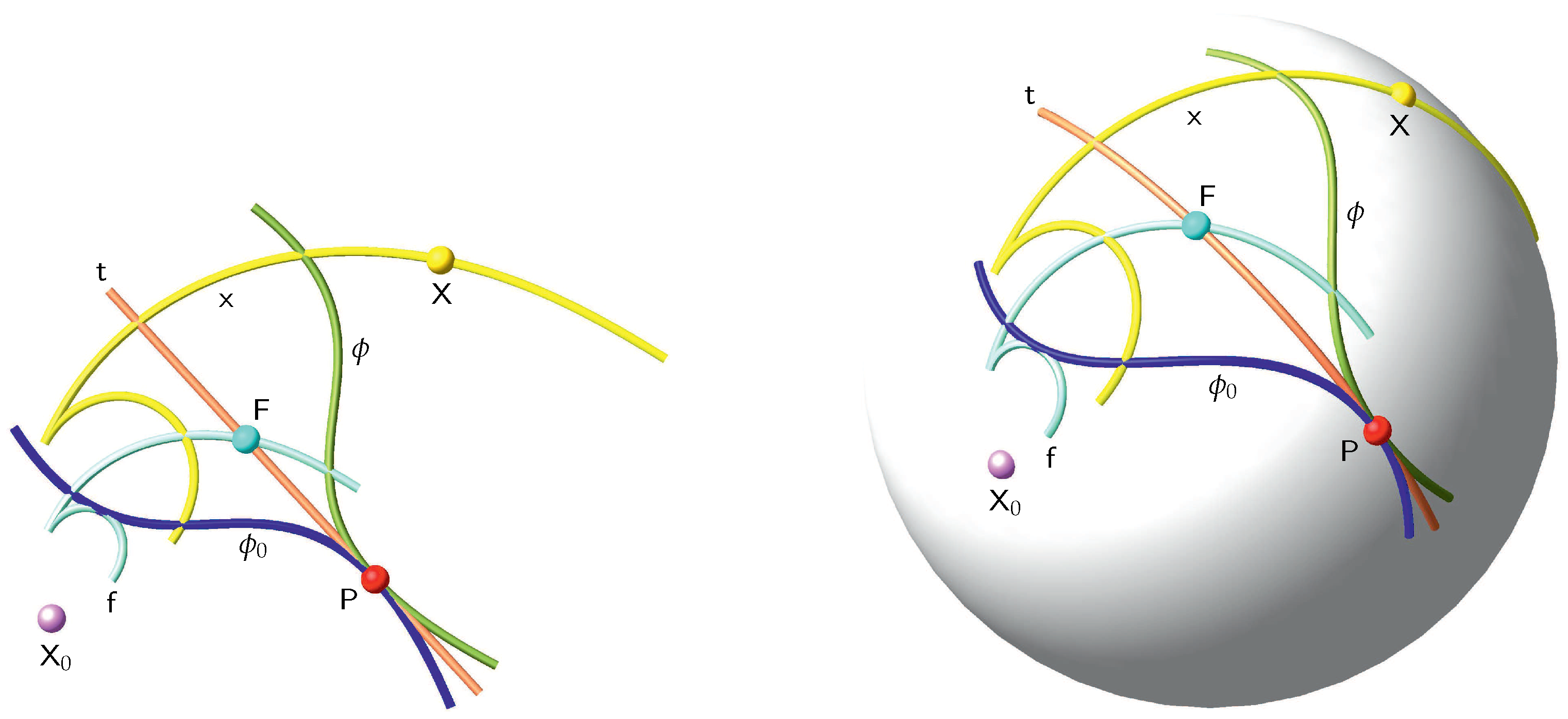
In planar kinematics, the instantaneous pole traces the so-called fixed/moving polode in the fixed/moving system during the constrained motion of a given mechanism. It is well known that this motion can also be generated by the rolling of the moving polode along the fixed polode without sliding. If the polodes are symmetric with respect to the pole tangent , then the motion is called planar symmetric rolling (cf. Figure 1, left). In 1826, this motion was first (with the exception of the already known symmetric circle rolling yielding the limacons of Pascal) studied by Quetelet [1], who pointed out the following property (cf. [2]): The path of a point under this special planar motion can be generated by the reflexion of a point of the fixed system on each tangent of . This can also be reformulated as follows: can be obtained by a central dilation with center and scale factor 2 (i.e., central doubling) of ’s pedal-curve with respect to . A detailed study of the planar symmetric rolling was done by Bereis [3], Bottema [4] and Tölke (cf. [2] and the references given therein).
The spherical counterpart of this motion is called spherical symmetric rolling and was extensively studied by Tölke in a series of papers, which are summarized and referenced in [2]. The spherical version of the above given characterization also holds true for the spherical symmetric rolling (cf. Figure 1, right).
From another perspective, a planar/spherical symmetric rolling can also be generated by reflecting the fixed system in a 1-parametric continuous set of lines/great circles. This point of view is of importance for the spatial generalization of symmetric rollings, which can be done in multiple ways:
- Darboux noted in [5] (No. 61) a 2-parametric spatial motion, which is generated by the rolling of a moving surface on an indirect congruent fixed surface . It also holds that the path-surface of a point can be generated by the reflexion of a point of the fixed system on each tangent-plane of ; for example, the path-surface can be obtained by a central doubling of ’s pedal-surface with respect to ’s tangent-planes.
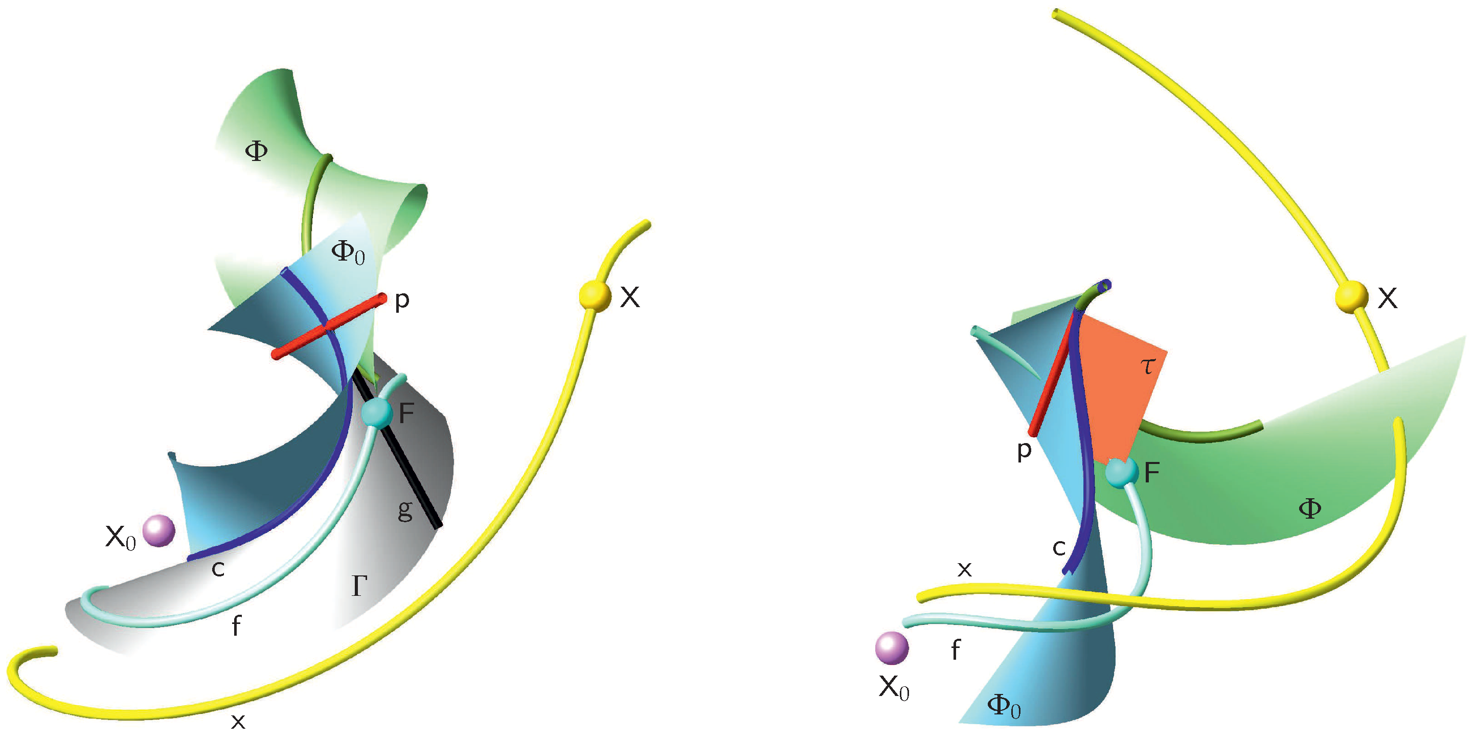
- Krames [6] considered the so-called line-symmetric motion as the 1-parametric spatial analogue of the planar/spherical symmetric rolling. These motions are obtained by reflecting the moving system in a 1-parametric continuous set of lines, which form the so-called basic surface (cf. Figure 2, left). Krames reasoned this by the fact that the path of a point under a line-symmetric motion can be generated by the reflexion of a point on each generator of ; for example, can be obtained by a central doubling of ’s pedal-curve with respect to ’s rulings. However, it should be pointed out that differs from the fixed axode (generated by the central tangents of ). However, and the moving axode are at each time instant symmetric with respect to the axis of the instantaneous screw, which is in general not an instantaneous rotation. For further details and references on this motion type, please see [7,8] (§7 of Ch. 4) and [9].
- It is astonishing that neither Tölke [2] (Section 3.1) nor Krames [6] (p. 394) mentioned the more apparent generalization by reflecting the fixed system in a 1-parametric continuous set of planes. Less attention was paid to these so-called plane-symmetric motions in the literature until now. We summarize the known results in the next section.
Remark 1.
Note that the term plane-symmetric motion was also used in [10] (§3.3) for a superset of the above described motions, which is characterized by the sole property that "the same equation describes the motion and its inverse, but with respect to reference systems that are a reflection of each other". In order to avoid confusions, we point out that we do not mean this superset by using this wording.
1.1. Review on Plane-Symmetric Motions
The basic properties of this motion type are reported in [8] (§8 of Ch. 4). Given is a 1-parametric continuous set of planes , where the parameter t can be seen as time. By reflecting the fixed frame on the plane we obtain the pose of the plane-symmetric motion.
Let us consider to infinitesimal neighboring poses and of the plane-symmetric motion. Now, one can transform into by a reflexion on followed by a further reflexion on . It is well known that this is a pure rotation about the line of intersection of and . Moreover, this is exactly a torsal ruling of the developable surface enveloped by the given 1-parametric set of planes. As a consequence, the fixed axode is a developable surface (It is well known (e.g., [11] (Thms. 5.1.7 and 6.1.3)) that every developable surface is composed of cylindrical, conical or tangent-surfaces) and the corresponding moving axode is obtained by reflecting in ’s tangent-plane along the instantaneous axis of rotation (cf. Figure 2, right). Now, the path of a point under a plane-symmetric motion can be generated by the reflexion of a point on each tangent-plane of ; i.e., can be obtained by a central doubling of ’s pedal-curve with respect to ’s tangent-planes.
Due to all these properties, the plane-symmetric motion seems to be the straightforward spatial counterpart of the planar/spherical symmetric rolling. Therefore, we call a plane-symmetric motion also a spatial symmetric rolling.
As far as the author knows, these spatial symmetric rollings are only explicitly mentioned in a practical example by Kunze and Stachel [12], who pointed out that the relative motion of opposite systems of a threefold-symmetric Bricard linkage (e.g., the invertible cube of Schatz) is a plane-symmetric one. Clearly, this also holds for the more general class of plane-symmetric Bricard linkages [13], where the two opposite systems not containing a rotation-axis spanning the plane of symmetry also possess a plane-symmetric relative motion during the overconstrained motion of the closed 6R-chain.
1.2. Motivation and Outline
One of the author’s main research interests are hexapods with self-motions, i.e., overconstrained parallel manipulators where the platform is linked with the base by six legs, which are anchored via spherical red joints (Due to the spherical joints at the platform and the base, each leg can rotate about its carrier line without changing the pose of the platform. These uncontrolled leg-movements are not meant by the term self-motion). All these mechanical devices are solutions to the still unsolved problem posed by the French Academy of Science for the Prix Vaillant of the year 1904, which is also known as Borel–Bricard problem and reads as follows [14]: "Determine and study all displacements of a rigid body in which distinct points of the body move on spherical paths." In order to avoid trivial solutions of the problem, the following assumption should hold for the remainder of the article.
Assumption 1.
The platform anchor points of the hexapod as well as the corresponding base anchor points should span in each case at least a plane.
It is well known that so-called architecturally singular hexapods (A hexapod is called architecturally singular if the six legs belong in each relative pose of the platform with respect to the base to a linear line complex) possess self-motions in each pose (over ). These special solutions to the Borel–Bricard problem are already well studied (A review on this topic is given in [15] (Section 3.1)). The approaches for the determination of non-architecturally singular hexapods recorded in the literature (Note that we do not claim that the following list of given references is complete), can roughly be divided into the following two groups:
- Assumptions on the geometry of the platform and base; e.g.,
- (a)
- (b)
- (c)
- special topology (e.g., octahedral structure [25]),
- Assumptions on the self-motion; e.g.,
Note that these assumptions are done in order to reduce the complexity of the problem, as one has to deal with 30 design parameters (24 for the geometry and six leg lengths, whereby the number of 30 can be reduced by one due to the freedom of scaling) and six degrees of freedom.
We want to follow the second approach by assuming that the self-motions are symmetric rollings. Therefore, this paper closes a gap as line-symmetric self-motions and point-symmetric (Point-symmetric motions are obtained by reflecting the fixed system in a 1-parametric continuous set of points and according to [7] (Section 8), these motions are pure translations) self-motions are already well-studied [9,28]. In addition, this motion-type seems to be a good candidate for self-motions, due to the following property implied by the symmetry of the motion:
Theorem 1.
If a point of the moving system traces a spherical curve with center during a plane-symmetric motion, then also the point of the moving system has a spherical trajectory about the point , where and as well as and , are plane-symmetric points of the moving and fixed frame with respect to the tangent-plane τ along the instantaneous axis of rotation. As a consequence, the set of points with spherical trajectories is indirectly congruent to the set of corresponding sphere centers.
In the remainder of the paper, we call the replacement of the point pair by the “symmetric leg-replacement”.
Remark 2.
Clearly, the lower dimensional version of Theorem 1 is also true for the planar/spherical symmetric rolling. Moreover, Theorem 1 also holds for point-symmetric motions, if "plane-reflection" is substituted by "point-reflection". A similar result holds for line-symmetric motions; one only has to replace "plane-reflection" by "line-reflection" and "indirectly congruent" by "directly congruent" (see e.g., [9]).
The paper is structured as follows: We start with the discussion of planar/spherical symmetric rolling motions with circular paths in Section 2.1. In Section 2.2, we formulate the problem of determining hexapods with plane-symmetric self-motions in terms of algebraic geometry by means of Study parameters. Based on this description, the problem is solved in Section 3. One of the obtained solutions is the so-called Duporcq hexapod, which is discussed in more detail in Section 4. The paper is closed by a conclusion (cf. Section 5).
2. Preliminary Considerations and Preparatory Work
As far as the author knows, no hexapods with plane-symmetric self-motions are reported in the literature so far. From known results in planar/spherical kinematics, which are reviewed in the next subsection, we can immediately construct such hexapods.
2.1. Planar/Spherical Symmetric Rollings with Circular Paths
Clearly, a pure rotation is a planar/spherical symmetric rolling where every point of the moving system traces a circle. Besides this trivial case, which we meet again under the notation of a so-called butterfly self-motions (cf. later given Theorem 4), the following planar/spherical symmetric rollings with circular trajectories exist:
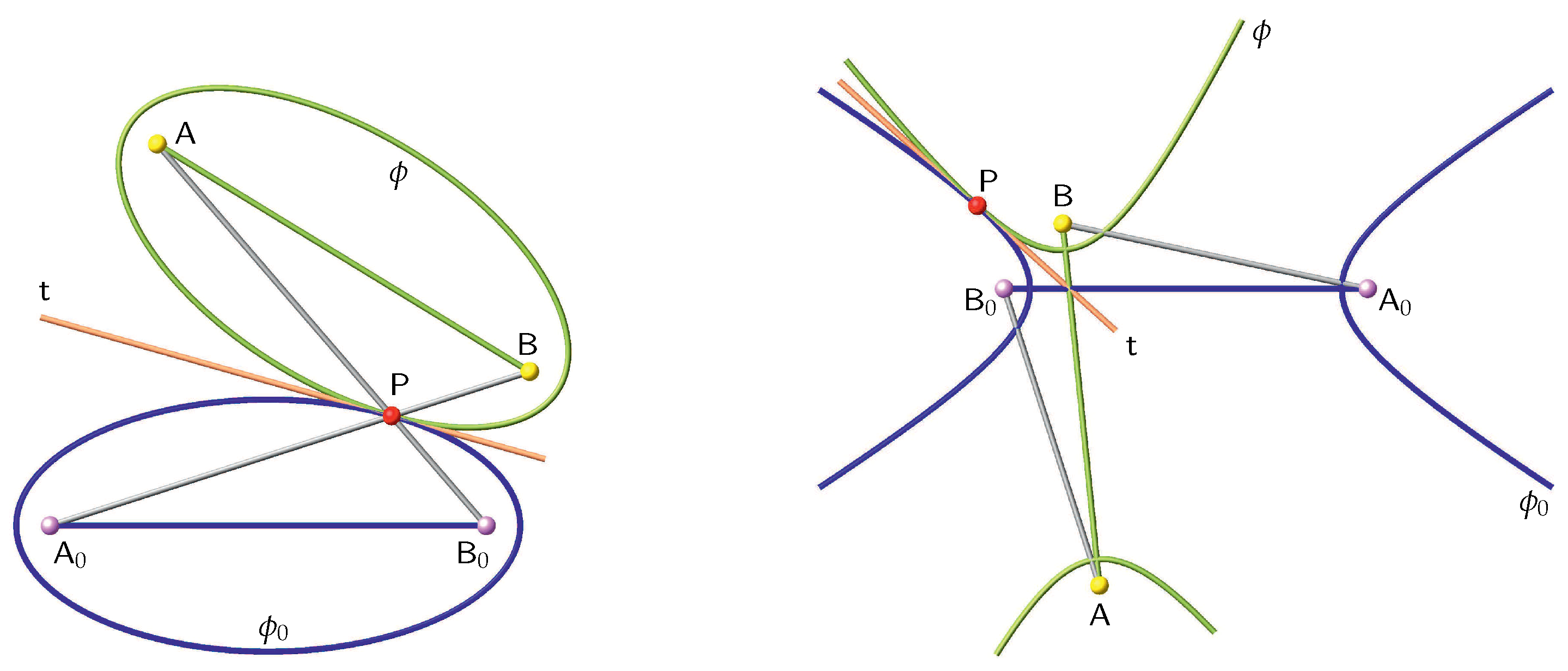
- The planar symmetric rolling motions with points running on circular paths are well known due to the study of Bereis [3]. In this case, the polodes are either ellipses or hyperbolas and the focals (two real, two complex) of the moving ellipse/hyperbola are running on circles. They are the Burmester points of this motion. These motion can be realized by the mechanisms illustrated in Figure 3.
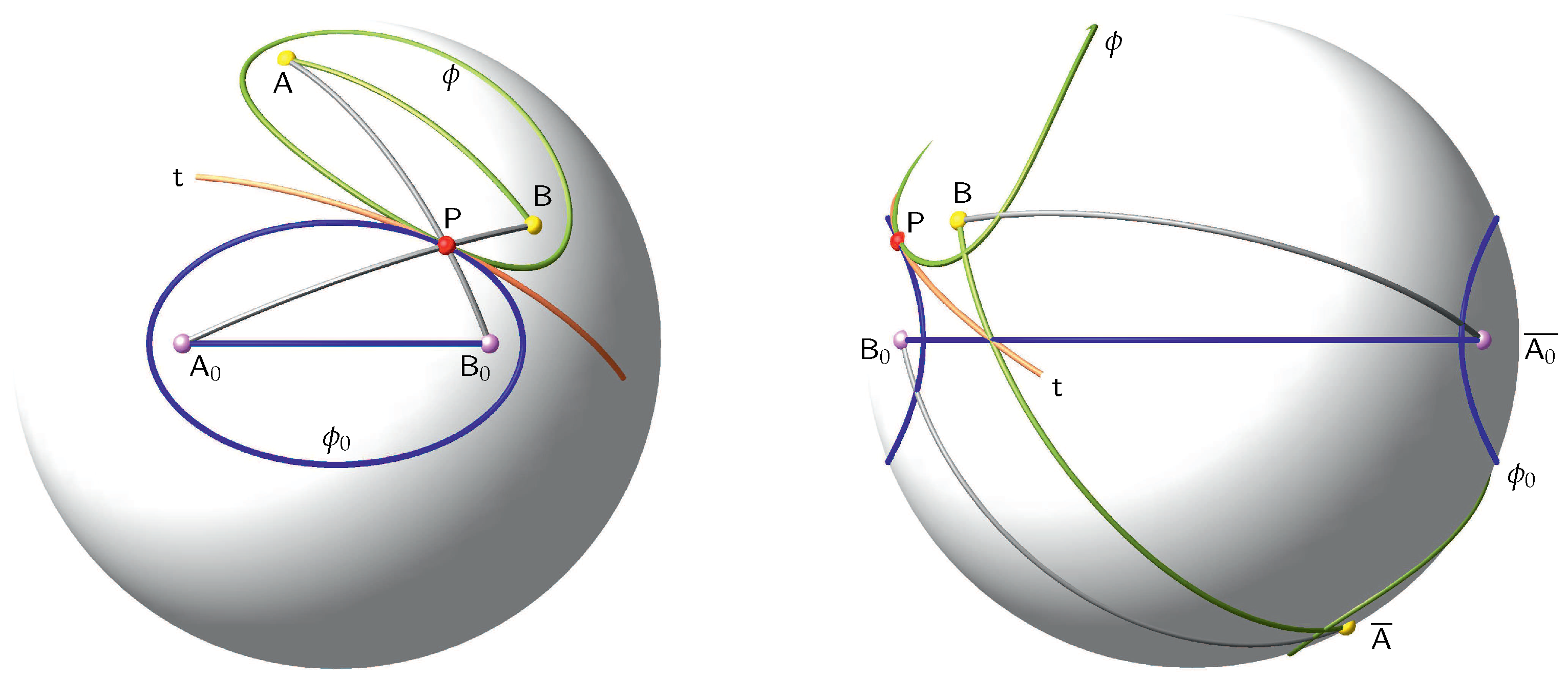
- Unfortunately, the considerations of Bereis cannot be generalized straightforward to the sphere (cf. [2] (p. 195)), as in spherical kinematics six Burmester points exist (e.g., [8] (p. 216)). However, we can do the reasoning in a different way. Due to [28] (Theorem 6), one can assume without loss of generality that only two points of a moving body can have spherical trajectories. According to the spherical version of Theorem 1, a second point is also running on a circle due to the symmetric leg-replacement (With the exceptional case that the first leg is orthogonal to the pole tangent, but this will not yield a closed loop; i.e., a spherical parallel manipulator). Thus, we can only end up with a spherical isogram illustrated in Figure 4, which is studied in more detail in [34].
From the discussed planar and spherical case, one can easily construct hexapods with plane-symmetric self-motions (see Figure 5).
Remark 3.
Note that the hexapods of Figure 5 do not only possess the illustrated plane-symmetric self-motions, but also the already mentioned butterfly self-motions (cf. later given Theorem 4).
2.2. Mathematical Framework
For the algebraic formulation of our problem, we want to use Study parameters , which are nothing else than homogenized dual unit-quaternions + with
where are the well-known quaternionic units and the dual unit with the property .
Now, all real points of the seven-dimensional Study parameter space , which are located on the so-called Study quadric , correspond to a Euclidean displacement with exception of the three-dimensional subspace E of given by , as its points cannot fulfill the condition with . The translation vector and the rotation matrix of the corresponding Euclidean displacement are given by:
and
if the normalizing condition is fulfilled.
Clearly, the reflection on a plane is an orientation-reversing congruence transformation, which cannot be described directly by the Study parameters. Therefore, we follow the approach of Selig and Husty [7] (Section 8), which is as follows: We start with a reflexion on a fixed plane; say the -plane of the fixed frame . By this plane-reflection of , we obtain . In addition, we apply the reflexion on the plane , which finally yields the pose . As the composition of two plane-reflexions is again a direct congruence transformation, we can describe the plane-symmetric motions in this way. If and the -plane of are
- not parallel, then the composition is a rotation about the line of intersection,
- parallel, then the composition is a translation orthogonal to these planes.
This yields that the plane-symmetric motions are given by . Moreover, it should be noted that the Study condition is fulfilled identically, thus the set of plane-symmetric motions corresponds to a three-dimensional generator space P of which intersects E in a line. Based on this description, we analyze the relation between plane-symmetric motions and line-symmetric ones in the next theorem:
Theorem 2.
A plane-symmetric motion is also a line-symmetric one if and only if there exists a linear relation with between the remaining Study parameters.
Proof.
For the proof, we need an algebraic characterization of line-symmetric motions in terms of Study parameters. It is well-known that there always exist, a Cartesian frame in the moving system in a way that holds for a line-symmetric motion. Then, are the Plücker coordinates of the generators of the basic surface with respect to the fixed frame.
A change of the moving system can be achieved by a so-called right multiplication; i.e., ( + ) ∘ ( + ) where ∘ stands for the quaternionic multiplication. If we denote this product by + , the corresponding entries and read as follows (under consideration of ):
If holds, then we set , , and . For , we set , , , and . For both cases, we get , which finishes the sufficiency of the linear relation between .
Its necessity can also be seen from Equation (2), as without such a linear relation, the condition can only be fulfilled for , which yields a contradiction as has to differ from the zero-quaternion. ☐
A further important theorem in this context is the following:
Theorem 3.
A plane-symmetric motion is also a line-symmetric one if and only if it is a planar motion or a spherical motion.
Proof.
If the linear relation equals , then it can easily be checked by direct computations that the point is mapped to the point for all fulfilling . Therefore, is the center of the spherical motion.
If the linear relation equals , then it can easily be checked by direct computations that the direction is mapped to the direction for all fulfilling . Therefore, the direction remains fixed under the motion. Moreover, the translation vector is orthogonal to this direction, which already proves that the motion is planar. ☐
These two theorems imply the following statement:
Corollary 1.
If we embed the planar and spherical symmetric rollings into SE(3), then they can also be seen as line-symmetric motions.
Therefore, the self-motions of the hexapods illustrated in Figure 5 are plane-symmetric and line-symmetric at the same time. This raises also the question of whether self-motions exist, which are plane-symmetric but not line-symmetric. The answer is given within the next section.
3. Plane-Symmetric Self-Motions
The coordinate vector of the base point with respect to the fixed system is given by . The position of the corresponding platform anchor point is obtained by reflecting a point with fixed coordinates in a 1-parametric continuous set of planes . Instead of these reflexions, we use direct isometries based on the Study representation described in Section 2.2 (i.e., ). Therefore, the locus of the corresponding platform anchor point with respect to the fixed frame can be parametrized as with .
The condition that the point is located on a sphere centered in with radius is a quadratic homogeneous equation in the Study parameters according to Husty [36]. For our setup, this so-called sphere condition has the following form:
It corresponds to a quadric in the three-dimensional projective space with homogenous coordinates . The symmetric leg-replacement (cf. Theorem 1) can also easily be seen within this formula, as it is invariant under the following permutations: , , . Due to this symmetry, we only have to find spatial rolling motions where three points have a spherical trajectory. This means that the corresponding three quardrics , and of have to have a curve in common, which can be a
- straight line,
- conic section,
- cubic curve,
- quartic curve.
In the following subsections these cases are discussed separately.
3.1. Intersection Curve Is a Straight Line
It is well-known that straight lines in the Study quadric correspond with either rotations about a line or straight translations. As the second option is not possible due to the sphere condition, we are only left with the rotation case. In the first step, we ask under which conditions two quadrics and have a straight line in common.
- General Case: Let us assume that and hold. Clearly, the straight line in has to correspond with a rotation about the line spanned by and . Therefore, the line spanned by and generates either a hyperboloid, cone or cylinder of revolution with axis . Moreover, all these poses of the platform points have to be obtained by plane-reflexions of the points and , respectively. This already implies that the 1-parametric set of planes has to be a pencil of planes with axis . Therefore, the leg lengths and are given bywhich is already the necessary and sufficient condition for the two quadrics and to have a straight line in common.
- Special Case: As the case and cannot arise (legs are identical), we only have to discuss one further case due to the symmetric leg-replacement. Without loss of generality, we can assume and . Now, has to trace a circle about the line , which in fact implies the same condition given in Equation (4) for .
Under consideration of the notation that and are coupled by the symmetric leg-replacement (for ), we can immediately formulate the following theorem.
Theorem 4.
Up to symmetric leg-replacements, the three quadrics , and have a line in common if and only if Equation (4) holds for and are collinear. The corresponding self-motion of the hexapod is a butterfly self-motion about the line spanned by , where holds for .
As these butterfly self-motions (cf. Figure 6, left) are trivial, they are not of further interest.
3.2. Intersection Curve Is a Conic
As the conic is a planar curve, there has to exist a linear relation between the homogenous coordinates of . Therefore, we can apply the Theorems 2 and 3, which imply that we can only end up with planar/spherical symmetric rollings already discussed in Section 2.1.
3.3. Intersection Curve Is Cubic
A necessary condition that , and have a cubic curve in common is that the intersection of two quadrics split up into a line and this cubic. Therefore, condition Equation (4) has to hold. It can easily be checked that splits up into two planes:
![Robotics 07 00027 g006]() under consideration of Equation (4). Therefore, the cubic has to split up into three lines, which all correspond to plane-symmetric butterfly self-motions already described in Theorem 4. As a consequence, no further discussion of this case is necessary.
under consideration of Equation (4). Therefore, the cubic has to split up into three lines, which all correspond to plane-symmetric butterfly self-motions already described in Theorem 4. As a consequence, no further discussion of this case is necessary.
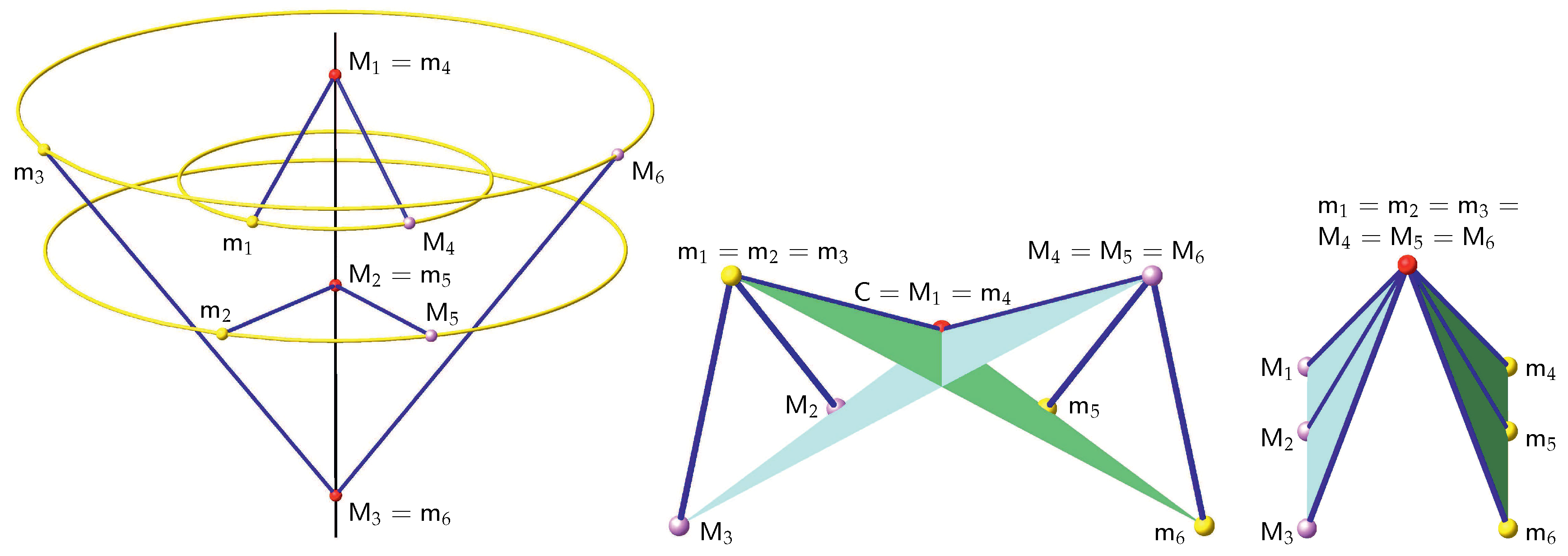
Figure 6.
In all three illustrations, the plane of symmetry is always a vertical projecting plane; left: butterfly self-motion of a hexapod. Note that not necessarily the three legs obtained by the symmetric leg-replacements have to be added, but any legs where neither or is collinear with for ; center: situation after performing the -transform; right: two-dimensional spherical self-motion.

3.4. Intersection Curve Is Quartic
We start with the following lemma, which helps to exclude the discussion of special cases arising.
Lemma 1.
If are collinear and holds (under consideration of symmetric leg-replacements), then the hexapod can only have the following plane-symmetric self-motions:
- 1.
- butterfly self-motion,
- 2.
- two-dimensional spherical self-motion,
- 3.
- planar/spherical symmetric rollings of Section 2.1.
Proof.
If the carrier line of is always identical with the reflected carrier line of , then it is clear that the motion can only be a butterfly motion (cf. Figure 6, left).
Moreover, it is trivial, that the motion can only be a planar one if is always parallel to (⇒ planar symmetric rolling of Section 2.1).
Now, we discuss the remaining case that, during the plane-symmetric self-motion, one configuration exists, where and intersect in one point . As the first three legs are always in a pencil of lines, one can make a so-called -transform [37] (without changing the self-motion) such that holds. This results in the following relations (cf. Figure 6, center):
Under consideration of the plane-symmetric setup, these conditions can only be fulfilled if
- holds, which yields the spherical symmetric rolling (with center ) of Section 2.1,
- holds, which implies a two-dimensional spherical self-motion (with center ; cf. Figure 6, right).
This finishes the proof. ☐
Remark 4.
If , and have a quadric curve in common, they are contained within a pencil of quadrics, which is already spanned by two of them. Therefore, we make the following ansatz:
In order to simplify the resulting direct computations, we can select the fixed frame in a clever way based on the following lemma:
Lemma 2.
By applying symmetric leg-replacements, we can assume that span a plane (under consideration of Assumption 1).
Proof.
If are collinear (span the line ), we apply the symmetric leg-replacement to the ith leg for . Due to Assumption 1, at least one of the are not located on , thus, after a renumeration of anchor points, the lemma holds. ☐
Due to Lemma 2, we can assume without loss of generality that the origin of the fixed frame equals , that is located on the positive -axis of the fixed frame and that is located in the -plane of the fixed frame for pairwise distinct . As is a triangle there always exist at least four (This number results from the fact that each triangle has at least two acute angles, whose two vertices can be used as ) choices for in a way that is located in the 1st quadrant of the -plane. After a may necessary renumeration, we can assume:
with , and . Moreover, by selecting the unit-length in a suitable way, we can achieve .
Based on this choice of the fixed frame, we inspect the coefficients of the linear combination given in Equation (7) with respect to the Study parameters. We denote the coefficient of by . From , we get . Moreover, we can compute from . Then, equals , which implies . From , we get . Now, yields . Then, we express and from and which results in
Moreover, we can set due to . Then, we are only left with the following two conditions arising from and , respectively:
Eliminating out of these equations by resultant method yields:
Therefore, we distinguish the following cases:
- For , Equation (10) imply and , respectively. imply the conditions of Lemma 1.
- For , Equation (10) imply . Then, the second and third leg are identical under consideration of symmetric leg-replacement.
- For , we have to distinguish two cases:
- (a)
- : now, the condition simplifies to . As implies a contradiction, we set . Then, Equation (10) imply , which results in the conditions of Lemma 1.
- (b)
- : Under this assumption, we can solve this equation for . A further two cases have to be distinguished:
- : If one solves this equation for , then Equation (10) implies for distinct . In both cases, we end up with the conditions of Lemma 1.
- : Under this assumption, we can solve the condition implied by Equation (10) for , which yields:It can easily be checked that the obtained solution corresponds to the hexapod’s platform and base illustrated in Figure 7, which are also known as Duporcq’s complete quadrilaterals [38]. In the remainder of the paper, this interesting solution, which is discussed/studied in more detail in the next section, is called Duporcq hexapod. Based on this notation, we can formulate the following theorem.
Theorem 5.
Besides the trivial cases mentioned in Lemma 1, the quadrics , and belong to a pencil if and only if they correspond to sphere conditions of three legs of a Duporcq hexapod (which are not identical under symmetric leg-replacements).
4. Duporcq Hexapod
Due to the results obtained in Section 3 and Theorems 2 and 3, we can conclude that only the Duporcq hexapod of Theorem 5 possesses plane-symmetric self-motions, which are neither planar nor spherical motions. Therefore, we discuss this hexapod in more detail in this section.
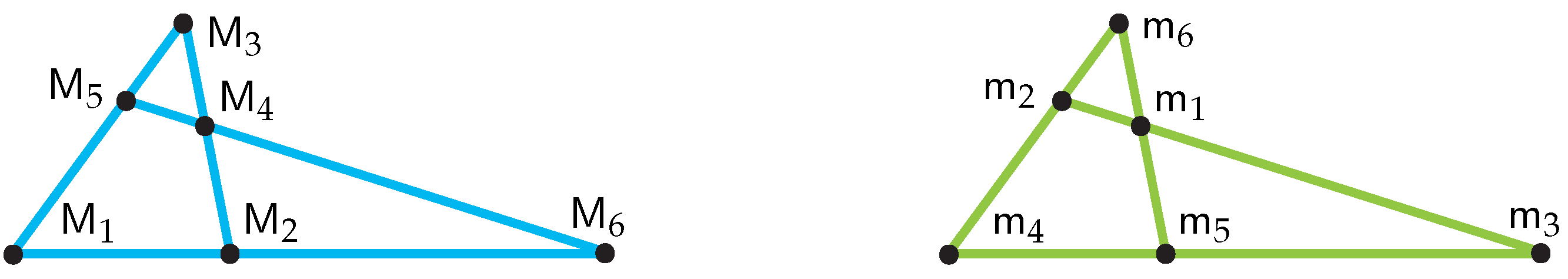
In [38], Duporcq describes the following remarkable motion: Let and be the vertices of two complete quadrilaterals, which are congruent. Moreover, the vertices are labeled in a way that is the opposite vertex of for (cf. Figure 7). Then, there exists a 2-parametric line-symmetric motion where each is running on spheres centered in .
It is well known [39] (Section 1) that this is an architecturally singular hexapod and that one can remove any leg without changing the direct kinematics of the mechanism. The resulting pentapod is called Duporcq pentapod and its line-symmetric self-motions were also studied in [39]. For the coordinatisation of the platform points and base points used in Section 3.4, the 2-parametric line-symmetric self-motion fulfills (cf. [39] (Section 4)).
Remark 5.
Note that the theoretic results of Section 4 are visualized on the basis of the following example:
This input data implies
with respect to the coordinatisation of the platform points and base points used in Section 3.4.
4.1. Plane-Symmetric Self-Motions of the Duporcq Hexapod
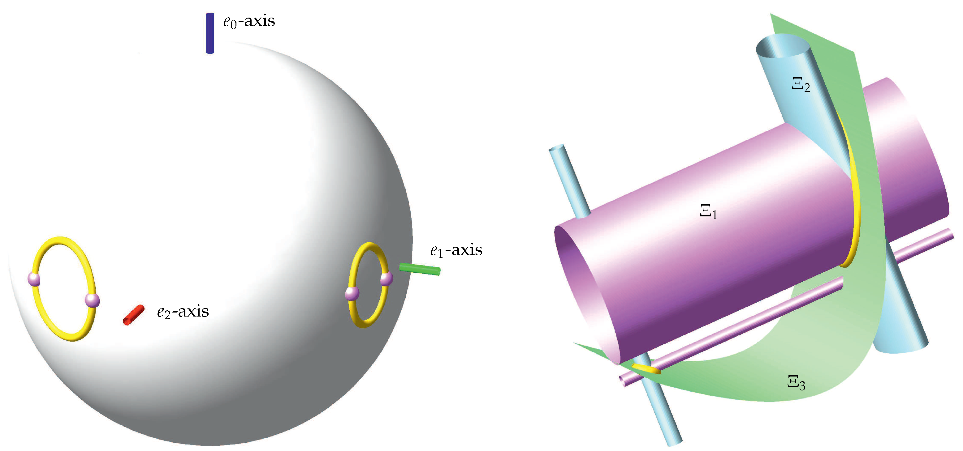
First of all, it should be pointed out that the plane-symmetric self-motions of the Duporcq manipulator were not known until now. They can be computed as follows: We express from the condition (which is linear in ). Plugging the resulting expression into implies a homogenous quartic equation in , which already represents the plane-symmetric self-motion (cf. Figure 8, left).
In the following, we are interested in the transition poses between this one-dimensional plane-symmetric self-motion and the above-mentioned two-dimensional line-symmetric one. Therefore, we only have to intersect the quartic curve with , which yields four of these so-called branching singularities [40]. These four transition poses are totally flat configurations of the Duporcq hexapod (cf. Table 1, Figure 8, red left and Figure 9).
Remark 6.
Note that a further prominent example of a hexapod, which possesses flat poses during its self-motion, is Bricard’s flexible octahedron of type 3 (cf. [41]).
Moreover, it should be mentioned that the Duporcq hexapod is a kinematotropic mechanism (according to the notation of Wohlhart [42]). To the best of the author’s knowledge, only one further hexapod with this property is known so far, which is the so-called Wren platform (see [42] (Section 3) and [21] (Section 2.2)).
For the example at hand, the fixed axode can be described in the dual representation (If is the equation of the plane of symmetry, then its dual representation is given by the homogenous quadruplet according to [11] (Section 6.2)) as the intersection of the following three surfaces displayed in Figure 8, right:
Based on these surfaces, it can be checked (e.g., by computing the Hilbert-polynomial) that the fixed axoide corresponds to an algebraic curve of degree 4 in the dual representation. This curve can easily be parametrized as follows (two branches):
with . Moreover it can be seen (cf. Figure 8, right) that the curve has two components. The left one is obtained for and the right one for . Note that the borders of the two intervals are the roots of w, which can be computed explicitly, but, in order to avoid too long expressions, we displayed them numerically.
4.2. Point-Symmetric Self-Motions of the Duporcq Hexapod
Finally, we want to correct a statement given in [39] (Remark 4), where it is stated that
- the Duporcq manipulator also has pure translational one-dimensional self-motions,
- each two-dimensional line-symmetric self-motion of a Duporcq manipulator contains a pure translational one-dimensional sub-self-motion.
The first statement is true in contrast to the second one. In fact, the pure translational self-motion (which can be considered as point-symmetric self-motion) has two branching singularities, where they can switch into a 2-parametric line-symmetric self-motion. This can easily be seen as follows:
For the coordinatisation of the platform points and base points used in Section 3.4, the 1-parametric point-symmetric motion fulfills . It can be computed by expressing from (which is linear in ). Plugging the resulting expression into implies a homogenous quadratic equation in , which already represents the point-symmetric self-motion. By the additional condition , we obtain the two mentioned branching singularities, which are again totally flat configurations of the Duporcq hexapod ( cf. Table 2 and Figure 11).
Finally it should be noted that there is no branching singularity between plane-symmetric self-motions and point-symmetric self-motions as has to hold, which contradicts the normalizing condition . Summed up one can say, that the Duporcq hexapod is a twofold kinematotropic mechanism, as there are branching singularities between the two-dimensional line-symmetric self-motion and the one-dimensional
- point-symmetric self-motion,
- plane-symmetric self-motion.
Due to its kinematotropic behavior and its total flat branching singularities the Duporcq manipulator is possibly of interest for the design of deployable structures.
5. Conclusions
This paper gives a complete classification of hexapods with plane-symmetric self-motions. It turns out that besides the planar/spherical symmetric rollings with circular paths and two trivial cases (butterfly self-motion and two-dimensional spherical self-motion), only one further solution exists, which is the so-called Duporcq hexapod. This is the only manipulator possessing plane-symmetric self-motions, which are neither planar nor spherical motions (and therefore also no line-symmetric motions). Moreover, the Duporcq hexapod is may be of interest for the design of deployable structures due to its kinematotropic behavior and total flat branching singularities.
Funding
The author is supported by Grant No. P 24927-N25 of the Austrian Science Fund FWF within the project “Stewart Gough platforms with self-motions”.
Conflicts of Interest
The author declares no conflict of interest.
References
- Quetelet, L.A.J. Memoire sur une nouvelle maniere de considerer les caustiques, produites soit par reflexion soit par refraction. Brux. Nouv. Mem. 1826, 3, 89–140. (In French) [Google Scholar]
- Tölke, J. Ebene euklidische und sphärische symmetrische Rollungen. Mech. Mach. Theory 1978, 13, 187–198. (In German) [Google Scholar] [CrossRef]
- Bereis, R. Über die symmetrische Rollung. Österr. Ing. Arch. 1953, 7, 243–246. (In German) [Google Scholar]
- Bottema, O. Characteristic properties of the symmetric plane motion. Proc. K. Ned. Akad. Wet. B 1972, 75, 145–151. [Google Scholar]
- Darboux, G. Lecons sur la Theorie Generale des Surfaces; Gauthier-Villars: Paris, France, 1887. (In French) [Google Scholar]
- Krames, J. Über Fußpunktkurven von Regelflächen und eine besondere Klasse von Raumbewegungen (Über symmetrische Schrotungen I). Monatsh. Math. Phys. 1937, 45, 394–406. (In German) [Google Scholar] [CrossRef]
- Selig, J.M.; Husty, M. Half-turns and line symmetric motions. Mech. Mach. Theory 2011, 46, 156–167. [Google Scholar] [CrossRef] [Green Version]
- Bottema, O.; Roth, B. Theoretical Kinematics; North-Holland: Amsterdam, The Netherlands, 1979. [Google Scholar]
- Gallet, M.; Nawratil, G.; Schicho, J.; Selig, J.M. Mobile Icosapods. Adv. Appl. Math. 2017, 88, 1–25. [Google Scholar] [CrossRef]
- Hernandez-Gutierrez, I. Screw Surfaces in the Analysis and Synthesis of Mechanisms. Ph.D. Thesis, Stanford University, Stanford, CA, USA, 1989. [Google Scholar]
- Pottmann, H.; Wallner, J. Computational Line Geometry; Springer: Berlin/Heidelberg, Germany, 2001. [Google Scholar]
- Kunze, S.; Stachel, H. Über ein sechsgliedriges räumliches Getriebe. Elem. Math. 1974, 29, 25–32. (In German) [Google Scholar]
- Baker, J.E. The single screw reciprocal to the general plane-symmetric six-screw linkage. J. Geom. Graph. 1997, 1, 5–12. [Google Scholar]
- Husty, M.E. Borel’s and R. Bricard’s Papers on Displacements with Spherical Paths and their Relevance to Self-Motions of Parallel Manipulators. In Proceedings of the International Symposium on History of Machines and Mechanisms–HMM 2000; Ceccarelli, M., Ed.; Kluwer: Dordrecht, The Netherlands, 2000; pp. 163–171. [Google Scholar]
- Nawratil, G. Correcting Duporcq’s theorem. Mech. Mach. Theory 2014, 73, 282–295. [Google Scholar] [CrossRef] [PubMed]
- Karger, A. Singularities and self-motions of equiform platforms. Mech. Mach. Theory 2001, 36, 801–815. [Google Scholar] [CrossRef]
- Karger, A. Singularities and self-motions of a special type of platforms. In Advances in Robot Kinematics: Theory and Applications; Lenarcic, J., Thomas, F., Eds.; Kluwer: Dordrecht, The Netherlands, 2002; pp. 155–164. [Google Scholar]
- Karger, A. Parallel manipulators with simple geometrical structure. In Proceedings of the EUCOMES 08: The Second European Conference on Mechanism Science; Ceccarelli, M., Ed.; Springer: Dordrecht, The Netherlands, 2008; pp. 463–470. [Google Scholar]
- Nawratil, G. Non-existence of planar projective Stewart Gough platforms with elliptic self-motions. In Computational Kinematics: Proceedings of the 6th International Workshop on Computational Kinematics (CK2013); Thomas, F., Perez Garcia, A., Eds.; Springer: Dordrecht, The Netherlands, 2013; pp. 49–57. [Google Scholar]
- Nawratil, G. On equiform Stewart Gough platforms with self-motions. J. Geom. Graph. 2013, 17, 163–175. [Google Scholar]
- Nawratil, G. Congruent Stewart Gough platforms with non-translational self-motions. In Proceedings of the 16th International Conference on Geometry and Graphics; Schröcker, H.-P., Husty, M., Eds.; Innsbruck University Press: Innsbruck, Austria, 2014; pp. 204–215. [Google Scholar]
- Nawratil, G. On the Self-Mobility of Point-Symmetric Hexapods. Symmetry 2014, 6, 954–974. [Google Scholar] [CrossRef] [Green Version]
- Dietmaier, P. Forward kinematics and mobility criteria of one type of symmetric Stewart-Gough platforms. In Recent Advances in Robot Kinematics; Lenarcic, J., Parenti-Castelli, V., Eds.; Kluwer: Dordrecht, The Netherlands, 1996; pp. 379–388. [Google Scholar]
- Karger, A.; Husty, M. Classification of all self-motions of the original Stewart-Gough platform. Comput. Aided Des. 1998, 30, 205–215. [Google Scholar] [CrossRef]
- Nawratil, G. Self-motions of parallel manipulators associated with flexible octahedra. In Proceedings of the Austrian Robotics Workshop; Hofbaur, M., Husty, M., Eds.; Umit Lecture Notes: Hall in Tyrol, Austria, 2011; pp. 232–248. [Google Scholar]
- Nawratil, G. Planar Stewart Gough platforms with a type II DM self-motion. J. Geom. 2011, 102, 149–169. [Google Scholar] [CrossRef]
- Husty, M.L.; Karger, A. Self motions of Stewart-Gough platforms, an overview. In Proceedings of the Workshop on Fundamental Issues and Future Research Directions for Parallel Mechanisms and Manipulators, Quebec City, QC, Canada, 2–3 October 2002; Gosselin, C.M., Ebert-Uphoff, I., Eds.; pp. 131–141. [Google Scholar]
- Nawratil, G. Introducing the theory of bonds for Stewart Gough platforms with self-motions. ASME J. Mech. Rob. 2014, 6. [Google Scholar] [CrossRef]
- Gallet, M.; Nawratil, G.; Schicho, J. Liaison Linkages. J. Symb. Comput. 2017, 79, 65–98. [Google Scholar] [CrossRef]
- Borel, E. Mémoire sur les déplacements à trajectoires sphériques. In Mém. Présent. Var. Sci. Acad. Sci. Natl. Inst. Fr. TOME XXXIII; Imprimerie Nationale: Paris, France, 1908; pp. 1–128. (In French) [Google Scholar]
- Bricard, R. Mémoire sur les déplacements à trajectoires sphériques. J. École Polytech. 1906, 11, 1–96. (In French) [Google Scholar]
- Karger, A. New Self-Motions of Parallel Manipulators. In Advances in Robot Kinematics: Analysis and Design; Lenarcic, J., Wenger, P., Eds.; Springer: Dordrecht, The Netherlands, 2008; pp. 275–282. [Google Scholar]
- Karger, A. Self-motions of Stewart-Gough platforms. Comput. Aided Geom. Des. 2008, 25, 775–783. [Google Scholar] [CrossRef]
- Figliolini, G.; Angeles, J. The Spherical Equivalent of Bresse’s Circles: The Case of Crossed Double-Crank Linkages. ASME J. Mech. Rob. 2014, 9. [Google Scholar] [CrossRef]
- Glaeser, G.; Stachel, H.; Odehnal, B. The Universe of Conics; Springer Spektrum: Berlin/Heidelberg, Germany, 2016. [Google Scholar]
- Husty, M.L. An algorithm for solving the direct kinematics of general Stewart-Gough platforms. Mech. Mach. Theory 1996, 31, 365–380. [Google Scholar] [CrossRef]
- Borras, J.; Thomas, F.; Torras, C. On Delta Transforms. IEEE Trans. Robot. Autom. 2009, 25, 1225–1236. [Google Scholar] [CrossRef] [Green Version]
- Duporcq, E. Sur un remarquable déplacement à deux paramétres. Bull. Soc. Math. Fr. 1901, 29, 1–4. (In French) [Google Scholar]
- Nawratil, G.; Schicho, J. Duporcq Pentapods. ASME J. Mech. Rob. 2017, 9. [Google Scholar] [CrossRef]
- Gogu, G. Branching singularities in kinematotropic parallel mechanisms. In Computational Kinematics: Proceedings of the 5th International Workshop on Computational Kinematics; Kecskemethy, A., Müller, A., Eds.; Springer: Berlin/Heidelberg, Germany, 2009; pp. 341–348. [Google Scholar]
- Stachel, H. Flexible Polyhedral Surfaces With Two Flat Poses. Symmetry 2015, 7, 774–787. [Google Scholar] [CrossRef]
- Wohlhart, K. Kinematotropic linkages. In Recent Advances in Robot Kinematics; Lenarcic, J., Parenti-Castelli, V., Eds.; Kluwer: Dordrecht, The Netherlands, 1996; pp. 359–368. [Google Scholar]
Figure 1.
Sketch of the planar symmetric rolling (left) and the spherical symmetric rolling (right). The pedal-point of the fixed point with respect to the pol-tangent is denoted by .
Figure 1.
Sketch of the planar symmetric rolling (left) and the spherical symmetric rolling (right). The pedal-point of the fixed point with respect to the pol-tangent is denoted by .

Figure 2.
Sketch of the line-symmetric motion (left) and the spatial symmetric rolling (right). For the illustrations, the basic surface of the line-symmetric motion and the fixed axode of the spatial symmetric rolling have been chosen as tangent-surfaces of a straight cubic circle . denotes the pedal-point of the fixed point with respect to (left) the generator of and (right) the tangent-plane along the instantaneous axis of rotation, respectively.

Figure 3.
Twin-crank mechanisms with non-counter-rotating cranks (left): In this case, the polodes are ellipses. Twin-crank mechanism with counter-rotating cranks (right): In this case, the polodes are hyperbolas.
Figure 3.
Twin-crank mechanisms with non-counter-rotating cranks (left): In this case, the polodes are ellipses. Twin-crank mechanism with counter-rotating cranks (right): In this case, the polodes are hyperbolas.

Figure 4.
As on the sphere points can be replaced by their antipodes, it can easily be seen that every spherical conic can be interpreted as a spherical ellipse (e.g., [35] (Section 10.1)). The left and the right figure show the same symmetric rolling motion. If we replace and by their antipodal points and , respectively, and look on the sphere from the right side, then we get the figure illustrated on the right-hand side.

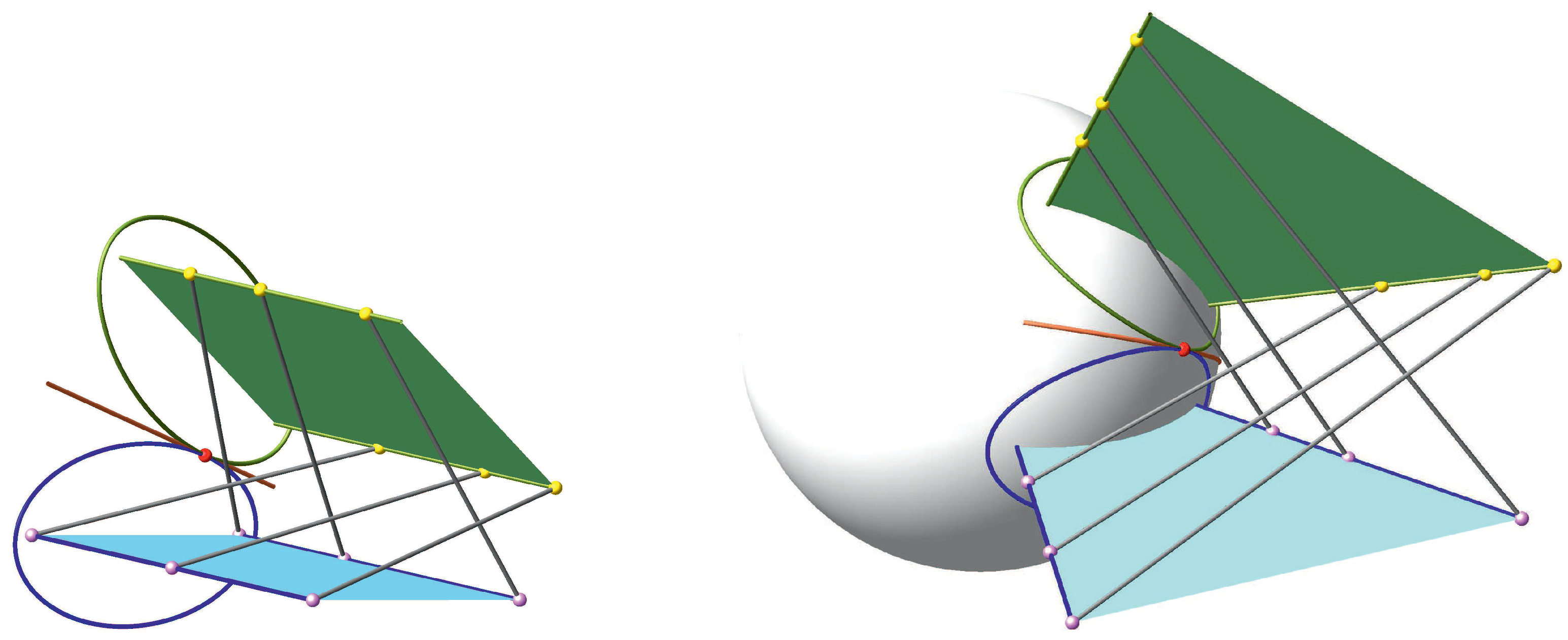
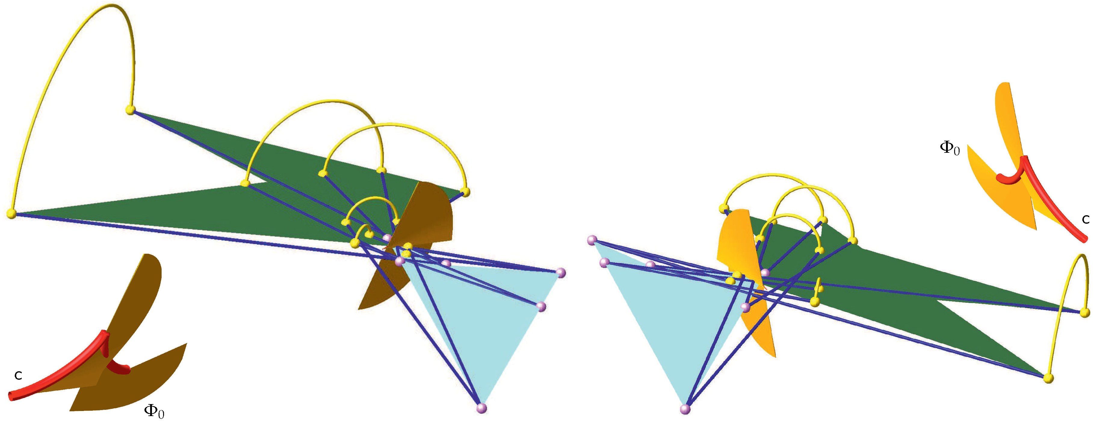
Figure 5.
Hexapods with plane-symmetric self-motions, where the platform (green) and the base (blue) are both planar. The axodes of the self-motions are cylinders (left) and cones (right), respectively, but we only illustrated the planar/spherical directrices of these singular quadrics to see better their connection to the planar/spherical symmetric rolling displayed in Figure 3 and Figure 4, respectively.

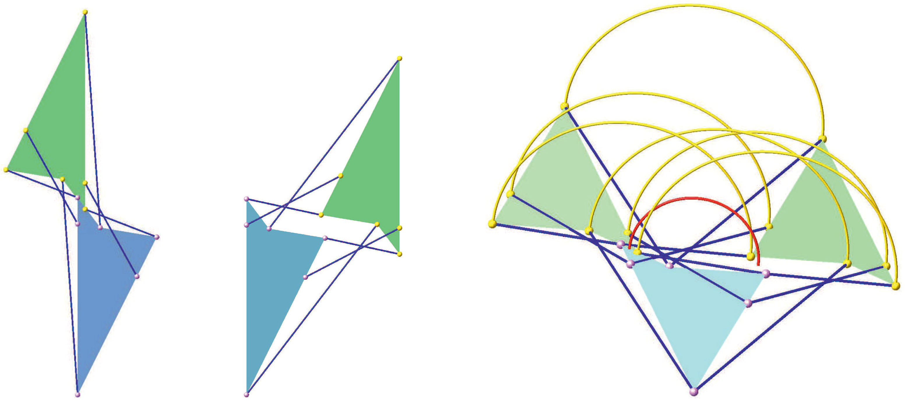
Figure 7.
Illustration of Duporcq’s complete quadrilaterals: The base (left) is congruent with the platform (right).
Figure 7.
Illustration of Duporcq’s complete quadrilaterals: The base (left) is congruent with the platform (right).

Figure 8.
(left:) the quartic is displayed under consideration of the normalization condition . For the example at hand, it consists of two components (as antipodal points yield the same displacement). Intersection points of the displayed spherical curve with the equator plane yield the branching singularities between plane-symmetric and line-symmetric self-motions. They are numbered from left to right by 1 to 4. (right): visualization of the surfaces under the assumption that corresponds to the ideal plane. The surface is a cylinder in direction of the -axis (for ).

Figure 9.
The four flat transition poses numbered from left to right by 1 to 4.

Figure 10.
Trajectories of the platform points during the plane-symmetric self-motion between the flat poses 1 and 2 (left) and the flat poses 3 and 4 (right). Moreover, the fixed axodes are displayed, which look like cones upon the first viewing. However, a blow up (in the lower left corner and upper right corner, respectively) of the region of the supposed vertex shows the line of regression of . For the illustrated self-motion, the tangents of in the two end points span the carrier plane (-plane) of the flat poses. If one considers the complete self-motion, then has four cusps (obtained by reflecting the illustrated curve at the -plane).

Figure 11.
The first and second flat pose (left and center, respectively) and the translational self-motion between them (right). This circular translation can also be seen as a point-symmetric motion, where the corresponding curve (half-circle) is illustrated in red.
Figure 11.
The first and second flat pose (left and center, respectively) and the translational self-motion between them (right). This circular translation can also be seen as a point-symmetric motion, where the corresponding curve (half-circle) is illustrated in red.


Table 1.
The Study parameters of the four flat transition poses illustrated in Figure 9. As they result as roots of a polynomial of degree 4, they can be computed explicitly, but, in order to avoid too long expressions, they are displayed numerically.
Table 1.
The Study parameters of the four flat transition poses illustrated in Figure 9. As they result as roots of a polynomial of degree 4, they can be computed explicitly, but, in order to avoid too long expressions, they are displayed numerically.
| Flat Pose | |||
|---|---|---|---|
| 1 | −0.63171148011492395006 | 0.77520358996267041460 | 0.24434973773984142590 |
| 2 | −0.26236530678800600560 | 0.96496862425367773706 | 0.36840718493416854565 |
| 3 | 0.89932040897259076870 | 0.43729029489044469464 | −1.6168042368274940498 |
| 4 | 0.98317707611585865513 | 0.18265496708349071532 | −2.3876030965525136289 |
Table 2.
The Study parameters of the two flat transition poses illustrated in Figure 11. As they result as roots of a polynomial of degree 2, they can be computed explicitly, but in order to avoid too long expressions they are again displayed numerically.
Table 2.
The Study parameters of the two flat transition poses illustrated in Figure 11. As they result as roots of a polynomial of degree 2, they can be computed explicitly, but in order to avoid too long expressions they are again displayed numerically.
| Flat Pose | |||
|---|---|---|---|
| 1 | 1 | 0.1406805116103807682 | −0.2234541534831142304 |
| 2 | 1 | 2.9246864608666834522 | −1.0586559382600050357 |
© 2018 by the author. Licensee MDPI, Basel, Switzerland. This article is an open access article distributed under the terms and conditions of the Creative Commons Attribution (CC BY) license (http://creativecommons.org/licenses/by/4.0/).
Share and Cite
MDPI and ACS Style
Nawratil, G. Hexapods with Plane-Symmetric Self-Motions. Robotics 2018, 7, 27. https://doi.org/10.3390/robotics7020027
AMA Style
Nawratil G. Hexapods with Plane-Symmetric Self-Motions. Robotics. 2018; 7(2):27. https://doi.org/10.3390/robotics7020027
Chicago/Turabian StyleNawratil, Georg. 2018. "Hexapods with Plane-Symmetric Self-Motions" Robotics 7, no. 2: 27. https://doi.org/10.3390/robotics7020027
Note that from the first issue of 2016, this journal uses article numbers instead of page numbers. See further details here.