
The Influence of Landscape Structure on Wildlife–Vehicle Collisions: Geostatistical Analysis on Hot Spot and Habitat Proximity Relations

Abstract
:1. Introduction
2. Materials and Methods
2.1. Study Area
2.2. Collision Data
2.3. Data Analysis
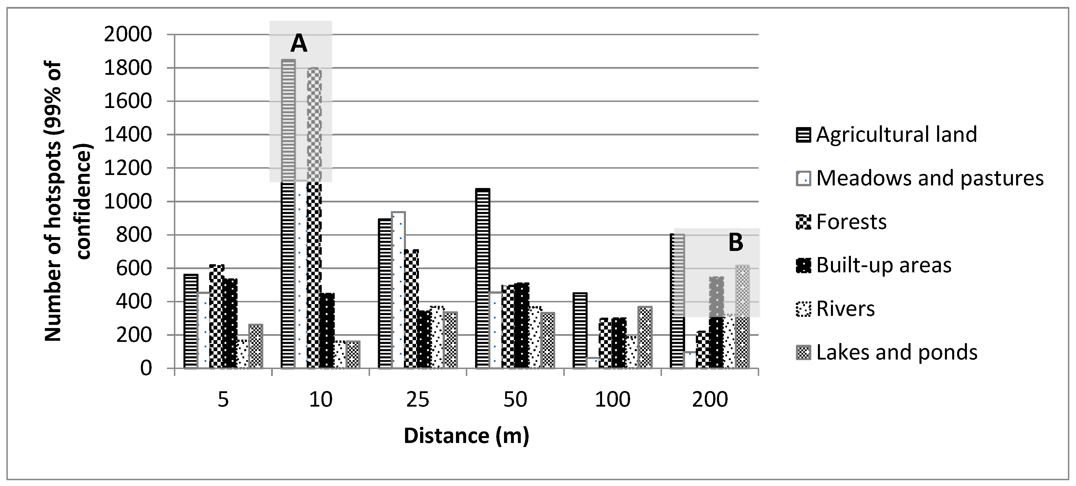
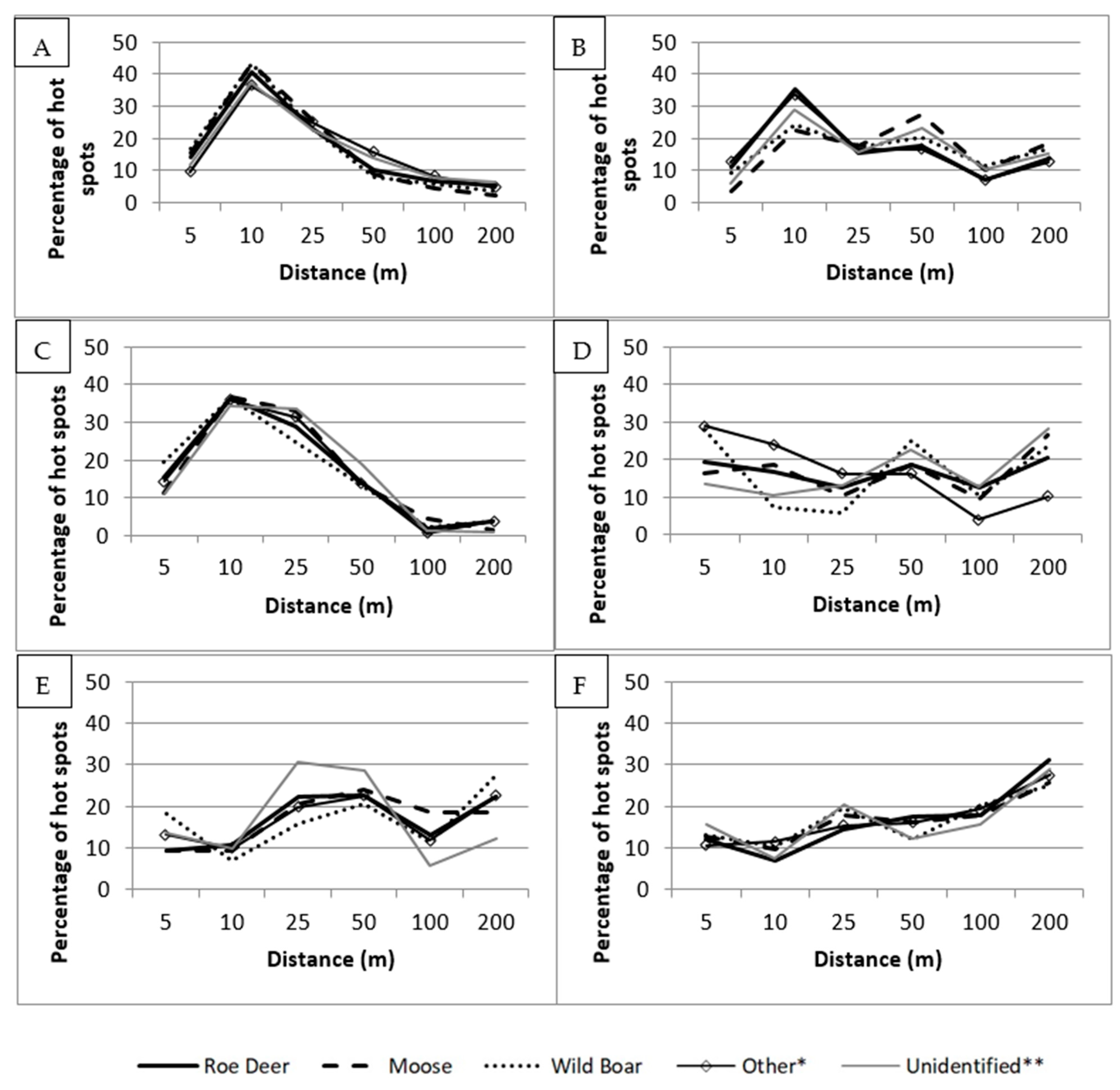
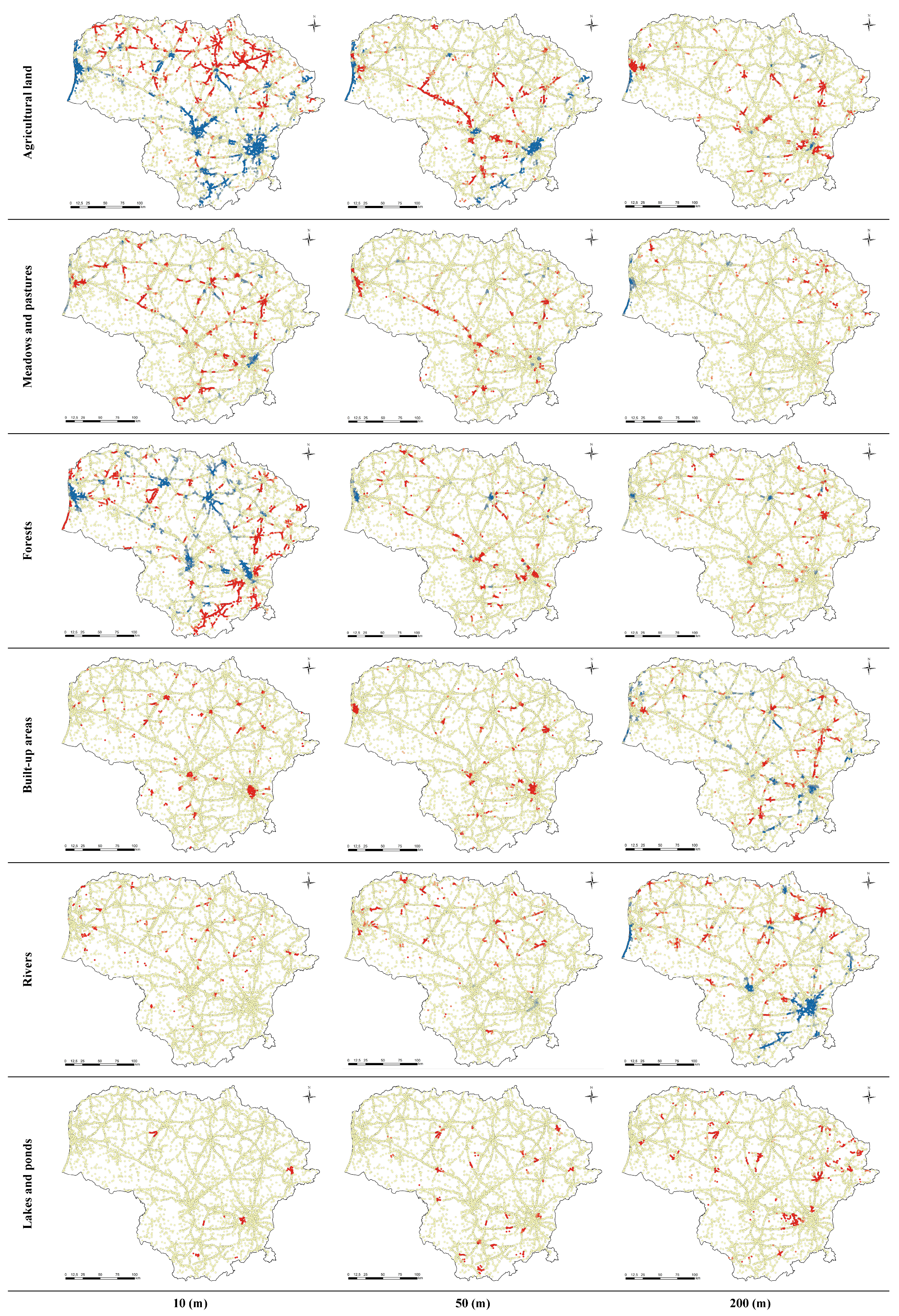
3. Results
4. Discussion
5. Conclusions
Author Contributions
Funding
Institutional Review Board Statement
Data Availability Statement
Acknowledgments
Conflicts of Interest
References
- Balčiauskas, L.; Jasiulionis, M. Reducing the incidence of mammals on public highways using chemical repellent. Balt. J. Road Bridge Eng. 2012, 7, 92–97. [Google Scholar] [CrossRef]
- Joyce, T.L.; Mahoney, S.P. Spatial and temporal distributions of moose-vehicle collisions in Newfoundland. Wildl. Soc. Bull. 2001, 29, 281–291. [Google Scholar] [CrossRef]
- Gunson, K.E.; Clevenger, A.P.; Ford, A.T.; Bissonette, J.A.; Hardy, A. A Comparison of Data Sets Varying in Spatial Accuracy Used to Predict the Occurrence of Wildlife-Vehicle Collisions. Environ. Manag. 2009, 44, 268–277. [Google Scholar] [CrossRef] [PubMed]
- Krisp, J.M.; Durot, S. Segmentation of lines based on point densities-An optimisation of wildlife warning sign placement in southern Finland. Accid. Anal. Prev. 2007, 39, 38–46. [Google Scholar] [CrossRef] [PubMed]
- Ramp, D.; Wilson, V.K.; Croft, D.B. Assessing the impacts of roads in peri-urban reserves: Road-based fatalities and road usage by wildlife in the Royal National Park, New SouthWales, Australia. Biol. Conserv. 2006, 129, 348–359. [Google Scholar] [CrossRef]
- Mountrakis, G.; Gunson, K.E. Multi-scale spatiotemporal analyses of moosevehicle collisions: A case study in northern Vermont. Int. J. Geogr. Inf. Syst. 2009, 23, 1389–1412. [Google Scholar] [CrossRef]
- Puglisi, M.J.; Lindzey, J.S.; Bellis, E.D. Factors associated with highway mortality of white-tailed deer. J. Wildl. Manag. 1974, 38, 799–807. [Google Scholar] [CrossRef]
- Hubbard, M.W.; Danielson, B.J.; Schmitz, R.A. Factors influencing the location of deer–vehicle accidents in Iowa. J. Wildl. Manag. 2000, 64, 707–713. [Google Scholar] [CrossRef]
- Clevenger, A.P.; Chruszczc, B.; Gunson, K.E. Spatial patterns and factors influencing small vertebrate fauna road-kill aggregations. Biol. Conserv. 2003, 109, 15–26. [Google Scholar] [CrossRef]
- Bíl, M.; Favilli, F.; Sedoník, J.; Andrášik, R.; Kasal, P.; Agreiter, A.; Streifeneder, T. Application of KDE+ software to identify collective risk hotspots of ungulate-vehicle collisions in South Tyrol, Northern Italy. Eur. J. Wildl Res. 2018, 64, 59. [Google Scholar] [CrossRef]
- Grilo, C.; Bissonette, J.; Santos-Reis, M. Spatial-temporal patterns in Mediterranean carnivore road casualties: Consequences for mitigation. Biol. Conserv. 2009, 142, 301–331. [Google Scholar] [CrossRef]
- Hoehun, H.; Fraser, S. Modelling potential wildlife-vehicle collisions (WVC) locations using environmental factors and human population density: A case-study from 3 state highways in Central California. Ecol. Inform. 2017, 43, 212–221. [Google Scholar] [CrossRef]
- Santos, S.M.; Lourenco, R.; Mira, A.; Beja, P. Relative effects of road risk habitat suitability, and connectivity on wildlife roadkills: The case of tawny owls (Strix aluco). PLoS ONE 2013, 8, e79967. [Google Scholar] [CrossRef] [Green Version]
- Snow, N.P.; Williams, D.M.; Porter, W.F. A landscape-based approach for delineating hotspots of wildlife-vehicle collisions. Landsc. Ecol. 2014, 29, 817–829. [Google Scholar] [CrossRef] [Green Version]
- Huijser, M.P.; McGowen, P.T.; Fuller, J.; Hardy, A.; Kociolek, A. Wildlife-Vehicle Collision Reduction Study: Report to Congress; FHWA-HRT-08-034; U.S. Department of Transportation, Federal Highway Administration: Washington, DC, USA, 2008; p. 254.
- Rodríguez-Morales, B.; Díaz-Varela, E.R.; Marey-Pérez, M.F. Spatiotemporal analysis of vehicle collisions involving wild boar and roe deer in NW Spain. Accid. Anal. Prev. 2013, 60, 121–133. [Google Scholar] [CrossRef]
- Shilling, F.M.; Waetjen, D.P. Wildlife-vehicle collision hotspots at US highway extents: Scale and data source effects. Nat. Conserv. 2015, 11, 41–60. [Google Scholar] [CrossRef] [Green Version]
- Langen, T.A.; Ogden, K.M.; Schwarting, L.L. Predicting hot spots of herpetofauna road mortality along highway networks. J. Wildl. Manag. 2009, 73, 104–114. [Google Scholar] [CrossRef]
- Gunson, K.E.; Mountrakis, G.; Quackenbush, L.J. Spatial wildlife-vehicle collision models: A review of current work and its application to transportation mitigation projects. J. Environ. Manag. 2011, 92, 1074–1082. [Google Scholar] [CrossRef] [PubMed]
- Bil, M.; Andrásik, R.; Janoska, Z. Identification of hazardous road locations of traffic accidents by means of kernel density estimation and cluster significance evaluation. Accid. Anal. Prev. 2013, 55, 265–273. [Google Scholar] [CrossRef]
- Galvonaitė, A.; Valiukas, D.; Kilpys, J.; Kitrienė, Z.; Misiūnienė, M. Climate Atlas of Lithuania; Lithuanian Hydrometeorological Service: Vilnius, Lithuania, 2013; pp. 8–15. [Google Scholar]
- Geoportal. Available online: https://www.geoportal.lt/geoportal/en/web/en/search#queryText=GRPK (accessed on 27 March 2021).
- Statistics of Fatal and Injury Road Accidents in Lithuania, 2014–2017. The Lithuanian Road Administration under the Ministry of Transport and Communications of the Republic of Lithuania. Available online: https://lakd.lrv.lt/lt/eismo-saugumas/eismo-ivykiu-statistika (accessed on 15 April 2021).
- Ministry of Environment of the Republic of Lithuania. Available online: https://am.lrv.lt/lt/veiklos-sritys-1/gamtos-apsauga/medziokle/medziojamuju-zveriu-apskaita (accessed on 10 May 2021).
- Getis, A.; Ord, J.K. The Analysis of Spatial Association by Use of Distance Statistics. Geogr. Anal. 1992, 24, 189–206. [Google Scholar] [CrossRef]
- Ord, J.K.; Getis, A. Local Spatial Autocorrelation Statistics: Distributional Issues and an Application. Geogr. Anal. 1995, 27, 286–306. [Google Scholar] [CrossRef]
- Mitchell, A. The ESRI Guide to GIS Analysis, 2nd ed.; ESRI Press: Redlands, CA, USA, 2005; pp. 161–187. [Google Scholar]
- Baleišis, R.; Bluzma, P.; Balčiauskas, L. Lietuvos Kanopiniai Žvėrys, 2nd ed.; Asveja: Vilnius, Lithuania, 1987. [Google Scholar]
- Hewison, A.J.M.; Vincent, J.P.; Joachim, J.; Angibault, J.M.; Cargnelutti, B.; Cibien, C. The effects of woodland fragmentation and human activity on roe deer distribution in agricultural landscapes. Can. J. Zool. 2001, 79, 679–689. [Google Scholar] [CrossRef]
- Borowik, T.; Cornulier, T.; Jędrzejewska, B. Environmental factors shaping ungulate abundances in Poland. Acta Theriol. 2013, 58, 403–413. [Google Scholar] [CrossRef] [PubMed] [Green Version]
- Ager, A.A.; Johnson, B.K.; Kern, J.W.; Kie, J.G. Daily and Seasonal Movements and Habitat Use by Female Rocky Mountain Elk and Mule Deer. J. Mammal. 2003, 84, 1076–1088. [Google Scholar] [CrossRef] [Green Version]
- Xie, S.; Marzluff, J.M.; Su, Y.; Wang, Y.; Meng, N.; Wu, T.; Gong, C.; Lu, F.; Xian, C.; Zhang, Y.; et al. The role of urban waterbodies in maintaining bird species diversity within built area of Beijing. Sci. Total Environ. 2022, 806, 150430. [Google Scholar] [CrossRef]
- Ancillotto, L.; Bosso, L.; Ramos, V.B.S.; Russo, D. The importance of ponds for the conservation of bats in urban landscapes. Landsc. Urban Plan. 2019, 190, 103607. [Google Scholar] [CrossRef]
- O’Brien, C.S.; Waddell, R.B.; Rosenstock, S.S.; Rabe, M.J. Widlife use of water catchments in Southeastern Arizona. Wildl. Soc. Bull. 2006, 34, 582–591. [Google Scholar] [CrossRef]
- Boroski, B.B.; Mossman, A.S. Distribution of mule deer in relation to water sources in Northern California. J. Wildl. Manag. 1996, 60, 770–776. [Google Scholar] [CrossRef]
- Found, R.; Boyce, M.S. Predicting deer-vehicle collisions in an urban area. J. Environ. Manag. 2011, 92, 2486–2493. [Google Scholar] [CrossRef]
- Zuberogoitia, I.; Real, J.; Torres, J.J.; Rodríguez, L.; Alonso, M.; Zabala, J. Ungulate Vehicle Collisions in a Peri-Urban Environment: Consequences of Transportation Infrastructures Planned Assuming the Absence of Ungulates. PLoS ONE 2014, 9, e107713. [Google Scholar] [CrossRef] [Green Version]
- Tajchman, K.; Drozd, L.; Karpiński, M.; Czyżowski, P.; Goleman, M.; Chmielewski, S. Wildlife—Vehicle collisions in urban area in relation to the behaviour and density of mammals. Pol. J. Natur. Sc. 2017, 32, 49–59. [Google Scholar]
- Litvaitis, J.A.; Tash, J.P. An Approach Toward Understanding Wildlife-Vehicle Collisions. Environ. Manag. 2008, 42, 688–697. [Google Scholar] [CrossRef] [PubMed]
- Ministry of Environment. Available online: http://senas.am.lt/VI/index.php#a/17724 (accessed on 5 April 2021).


| Species | Year | Total | ||||
|---|---|---|---|---|---|---|
| 2014 | 2015 | 2016 | 2017 | 2018 | ||
| Roe Deer | 1162/55.0 | 1352/55.8 | 1979/64.5 | 1561/65.2 | 2819/70.6 | 8873/63.4 |
| Moose | 160/7.6 | 183/7.6 | 210/6.8 | 173/7.2 | 260/6.5 | 986/7.1 |
| Wild Boar | 154/7.3 | 160/6.6 | 116/3.8 | 110/4.6 | 117/2.9 | 657/4.7 |
| Other * | 210/9.9 | 276/11.4 | 302/9.8 | 250/10.4 | 384/9.5 | 1422/10.2 |
| Unidentified ** | 425/20.2 | 452/18.6 | 459/15.1 | 300/12.6 | 414/10.5 | 2050/14.6 |
| Total | 2111/100.0 | 2423/100.0 | 3066/100.0 | 2394/100.0 | 3994/100.0 | 13,988/100.0 |
Publisher’s Note: MDPI stays neutral with regard to jurisdictional claims in published maps and institutional affiliations. |
© 2022 by the authors. Licensee MDPI, Basel, Switzerland. This article is an open access article distributed under the terms and conditions of the Creative Commons Attribution (CC BY) license (https://creativecommons.org/licenses/by/4.0/).
Share and Cite
Galinskaitė, L.; Ulevičius, A.; Valskys, V.; Samas, A.; Busher, P.E.; Ignatavičius, G. The Influence of Landscape Structure on Wildlife–Vehicle Collisions: Geostatistical Analysis on Hot Spot and Habitat Proximity Relations. ISPRS Int. J. Geo-Inf. 2022, 11, 63. https://doi.org/10.3390/ijgi11010063
Galinskaitė L, Ulevičius A, Valskys V, Samas A, Busher PE, Ignatavičius G. The Influence of Landscape Structure on Wildlife–Vehicle Collisions: Geostatistical Analysis on Hot Spot and Habitat Proximity Relations. ISPRS International Journal of Geo-Information. 2022; 11(1):63. https://doi.org/10.3390/ijgi11010063
Chicago/Turabian StyleGalinskaitė, Lina, Alius Ulevičius, Vaidotas Valskys, Arūnas Samas, Peter E. Busher, and Gytautas Ignatavičius. 2022. "The Influence of Landscape Structure on Wildlife–Vehicle Collisions: Geostatistical Analysis on Hot Spot and Habitat Proximity Relations" ISPRS International Journal of Geo-Information 11, no. 1: 63. https://doi.org/10.3390/ijgi11010063