Spatial–Temporal Data Imputation Model of Traffic Passenger Flow Based on Grid Division

Abstract

Traffic flows (e.g., the traffic of vehicles, passengers, and bikes) aim to reveal traffic flow phenomena generated by traffic participants in traffic activities. Various studies of traffic flows rely heavily on high-quality traffic data. The taxi GPS trajectory data are location data that include latitude, longitude, and time. These data are critical for traffic flow analysis, planning, infrastructure layout, and recommendations for urban residents. A city map can be divided into multiple grids according to the latitude and longitude coordinates, and traffic passenger flows data derived from taxi trajectory data can be extracted. However, random missing data occur due to weather and equipment failure. Therefore, the effective imputation of missing traffic flow data is a hot topic. This study proposes the spatio-temporal generative adversarial imputation net (ST-GAIN) model to solve the traffic passenger flows imputation. An adversarial game with multiple generators and one discriminator is established. The generator observes some components of the time-domain and regional traffic data vector extracted from the grid. It effectively imputes the missing values of the spatio-temporal traffic passenger flow data. The experimental data are accurate Kunming taxi trajectory data, and experimental results show that the proposed method outperforms five baseline methods regarding the imputation accuracy. It is significant and suggests the possibility of effectively applying the model to predict the passenger flows in some areas where traffic data cannot be collected for some reason or traffic data are randomly missing.

1. Introduction

Due to the rapid development of intelligent transportation, large amounts of valuable spatio-temporal traffic flow data are generated, including GPS trajectory data for taxis, buses, and shared motorbikes [1]. Several researchers have analyzed massive trajectory data to evaluate various traffic flows and real-time road conditions in a specific area or period. The travel patterns of urban residents have been investigated to guide urban transportation planning, infrastructure construction, and consumption [2]. However, trajectory data may have missing values due to weather conditions, failures of the positioning system, and building occlusion, resulting in incomplete collected data, which may mislead traffic analysis and management.

The generation of missingness in traffic data is a common phenomenon. Researchers typically refer to variables without missing values as complete variables and with missing values as incomplete variables. Three types of missing data problems have been identified [3]: (1) missing completely at random (MCAR) means that the reason for the missing data is not related to the data (incomplete and complete variables); (2) missing at random (MAR) indicates that the absence of data is not entirely random and depends on other complete variables; and (3) missing not at random (MNAR) implies that the missing data in the incomplete variable depend on the incomplete variable. Changes in the traffic flow data in adjacent areas can affect each other. For example, the traffic flow in an area adjacent to a missing data area is affected. As shown in Figure 1a, the missing flow value of road segment $s_3$ in period $t_4$ is correlated with the flow value of the adjacent road segment $s_2$ and $s_3$ in period $t_4$. The traffic flow in the previous time domain in a specific area affects the next time domain in the area. As shown in Figure 1b, the lack of flow in the continuous periods $t_4$ and $t_5$ in the road segment $s_1$ is related to the flow in periods $t_1$ to $t_3$. Therefore, the traffic flow data are MAR in most cases. It is crucial to use an effective data imputation method and correlation analysis of missing traffic flow data to achieve intelligent transportation in urban areas.

Data imputation is a way to deal with missing values in a dataset, usually using the correlation of known elements in the dataset to infer and fill in the missing values and improve the dataset’s quality to obtain better and more accurate results of data analysis [4]. Many techniques have been proposed for solving various missing traffic flow data. Most traffic data imputation methods utilize spatial, temporal, or spatio-temporal correlation between the data. Several statistical methods [5,6,7,8,9,10,11,12,13] and models have been proposed. Commonly used statistics used for imputation include the mean, weighted mean, or median for numerical data and the value of the largest category for categorical data. Some prediction models [14,15,16,17,18] predict the missing value utilizing information from existing values. Regression models [19,20,21,22,23] are used for the imputation of numerical variables, and classification models [24,25] are utilized for categorical variables. Researchers have exploited the spatio-temporal correlation of traffic data to construct a third-order flow tensor imputation model. The tensor with spatial and temporal dimensions has been used for tensor factorization [26] for the missing value imputation. Most researchers have used flow tensors to couple the spatio-temporal correlations [27,28,29] of traffic data and found that missing data imputation using tensor factorization was superior to most statistical-based methods. Machine learning techniques, especially deep learning models of the neural network, have been increasingly used in recent years to impute missing traffic data, providing good results [30]. Yoon et al. [31] first utilized a generative adversarial nets (GAN) [32] model for data imputation and proposed the generative adversarial imputation nets (GAIN) model, which achieved high imputation accuracy in missing values in the data vector.

Statistical methods often use the historical records of traffic data to impute missing values, which cannot deeply explore the traffic data’s spatial and temporal correlations and therefore have a lower performance. Models methods use tensor decomposition or deep learning to mine the correlation between traffic data from various dimensions, which usually achieves better results than statistical methods. The deep-learning-based model method has achieved better performance than the statistical and tensor model decomposition methods. Although deep learning performs well compared with other methods for missing traffic flow data, researchers still face the problem of not fully utilizing the correlation feature information between adjacent time and adjacent space of traffic flow data. In particular, when building the flow tensor, if the values in the tensor produced are missing randomly, rendering an incomplete tensor, the data similarity in the flow tensor is not fully utilized to impute the missing values, resulting in poor imputation results.

Aiming at the problem of random missing in the flow tensor, in this paper, we propose a traffic passenger flows imputation algorithm under the MAR assumption. We extract the pick-up points in taxi GPS trajectory data to construct a passenger flow tensor $\mathcal{N}\in \mathbb{R}i\times j\times s$ in a continuous period of the uniformly divided area; $i*j$ represents the grid division of the study region. The data in each grid represent the current time period (time period division, e.g., 11:00 to 12:00 as a time period), the number of pick-up points in this region is regarded as traffic passenger flows, and it is also a situation of traffic flow. $\mathcal{N}$ describes the flow change over time in s consecutive time periods in $i*j$ areas. The traffic distribution at the pick-up and drop-off points in taxi GPS trajectory data is representative of the traffic flow changes in an area. As shown in Figure 2, we select a representative period of three days (7, 10, 12, September 2019) in a part of the research area and visualize the distribution of pick-up and drop-off points on the real geographic grid, which shows that the pick-up and drop-off points are random, and the drop-off points are more centralized than the pick-up points. The number of pick-up points in each grid is not only more dispersed, but also the regional pick-up points flow further, reflecting the distribution of passenger flow demand. Therefore, selecting the pick-up points flow can more accurately simulate the random distribution of passenger demand within the region. This random distribution makes most of the grids that we divide contain a certain number of flow values, avoiding that only a small part of the grids contains flow values, resulting in a too concentrated distribution of flow values in the grids, thus making it difficult to mine the spatio-temporal correlation of passenger flow. We propose the missing traffic passenger flows data imputation model ST-GAIN based on spatio-temporal characteristics by introducing and improving the data imputation idea of the GAIN network. The problem of replacing missing data in the flow tensor is transformed into a data generation problem by minimizing the loss function. The improvement of this model is as follows:

(1) The new model observes the spatio-temporal correlation of the flow data vector. The flow tensor is unfolded into different flow matrices using different modes. Multiple generators with different weight parameters are used to simulate the vector components in different flow matrices. The flow matrix is restored to obtain a new flow tensor. The experimental results show that ST-GAIN can replace missing data and generate a result close to the real spatio-temporal traffic passenger flow distribution.

(2) We add a custom correlation loss to the loss item of the ST-GAIN model as part of the objective optimization function. The results of the ablation experiments demonstrate that this correlation loss term improves the model’s imputation performance.

The rest of this paper is organized as follows. Section 2 reviews the related work and explains the motivation for the study. Section 3 describes the proposed ST-GAIN method. Section 4 presents the experimental dataset, evaluation method, and experimental results. Section 5 concludes the paper and suggests topics for further research.

2. Literature Review

At present, the imputation methods of researchers for the missing traffic flow data in space and time mainly include imputation methods based on statistics, imputation methods based on tensor factorization models, and imputation methods based on deep learning models.

2.1. Data Imputation Based on Statistical Methods

Mazumder et al. [5] proposed a matrix-complete method, which used a convex algorithm to minimize the reconstruction error on the kernel norm to realize the missing values in the matrix completion. Royston and White [6] proposed a multiple imputation by chained equation (MICE), which used linear regression to perform multiple imputation on incomplete data. Stekhoven et al. [7] proposed an iterative imputation method (missForest) based on a random forest. Shi et al. [8] proposed a combined Bayesian principal component analysis and local least squares method to estimate missing values. Sha et al. [9] proposed a hybrid method for missing traffic data imputation based on the fuzzy C-means (FCM) [10], which is optimized by combining with other completion methods. The influence of multiple modes of traffic flow data is considered. Hong et al. [11] used the exponential smoothing method and the adjacent lane data weighting method to repair the missing problem in the traffic flow data. Song et al. [12] used an adaptive learning approach to learn a probabilistic regression model for each data tuple, and each tuple used the corresponding regression model to predict missing values. Tang et al. [13] proposed a hybrid model that combined adaptive network-based fuzzy inference system and fuzzy rough set to impute missing traffic data.

The traffic flow missing imputation based on statistical methods uses historical data to impute the current missing values. The performance of these methods depends on a priori estimation of the data distribution in the dataset. However, in many cases, the true distribution of traffic flow data is unknown, which leads to poor imputation performance.

2.2. Data Imputation Based on Tensor Factorization Models

Tan et al. [19] proposed a tensor-based traffic data imputation method for the first time. Based on the idea of coupled tensors, Zhou et al. [27] proposed an improved imputation method based on coupled matrix and tensor factorization (CMTF) to recover missing traffic data. Wu et al. [33] proposed an improved CP (CANDECOMP/PARAFAC) tensor factorization framework, which greatly improved the imputation performance of high missing rate data. Li et al. [28] used the tensor completion model to impute in the missing traffic data that indirectly improved the traffic flow prediction model. Cai et al. [29] used urban hotspots to introduce relevant information to impute in the missing areas based on CMTF. Yan et al. [20] proposed an imputation algorithm based on residual tensor factorization, which combined linear regression and CP factorization, and greatly improved the imputation accuracy. Chen et al. [21] proposed a low-rank autoregressive tensor model that uses the construction of a time-varying third-order tensor to capture the global consistency of traffic data, and experimentally demonstrated its effectiveness in diverse missing scenarios.

The traffic flow imputation model based on tensor factorization generally mines the internal characteristics of traffic data and analyzes the similarity and distribution pattern of the data. However, the existing methods require unfolding the original tensor into a matrix in the process of restoring the tensor, which leads to the loss of the correlation of some patterns in the constructed traffic tensor, thus reducing the imputation accuracy.

2.3. Data Imputation Based on Deep Learning Models

Che et al. [24] added gated recurrent units on the basis of the recurrent neural network (RNN) [34] to impute in time series data. Cao et al. [25] proposed a bidirectional long short-term memory (LSTM) to capture the data information before and after the current time point and improved the performance of data imputation. Li et al. [14] decomposed the input vector and combined LSTM and support vector machine to impute time series data through a multi-view method. Luo et al. [15] proposed to use the GAN network to perform missing value imputation for multivariate time series with a large number of missing values. Wang et al. [16] proposed a GAN-based road network traffic flow data imputation method. Zhang et al. [22] used LSTM to build a sequence-to-sequence model, and used the encoder–decoder structure for data imputation of time series. Luo et al. [17] combined a GAN and RNN variant gated recurrent unit network to build an end-to-end GAN network, and added the location information matrix of data missing points to impute time series data. Chen et al. [35] proposed a method that used parallel data and GAN to enhance traffic data imputation. Wang et al. [23] considered the temporal and spatial characteristics of traffic volume, and proposed a multilayer perceptron-multivariate imputation of chain equation (MLP-MICE) regression imputation method which combined multilayer perceptron and MICE, and further improved the use of MICE alone for imputation. Wang et al. [36] proposed a novel multi-view bidirectional spatio-temporal graph network, which comprehensively described traffic conditions from different temporal correlation views, and improved the loss function by considering the interactions between temporal correlation views, proving that the proposed method is suitable for traffic flow imputation with complex missing patterns. Yang et al. [18] proposed a spatio-temporal learnable bidirectional attention generative adversarial networks for missing traffic data imputation to improve imputation performance. Wang et al. [37] used a specific time-series analysis to mine periodic patterns and proposed a novel matrix decomposition method to describe the trend of the traffic flow data. Finally, the model built by fusing a novel dendritic neural network method greatly improved the imputation accuracy.

Data imputation methods based on deep learning usually have excellent imputation performance on spatio-temporal data and can well fit their distribution rules. However, when the dataset is too large, or the model is too complex, it will lead to a long training time and an overfitting problem.

3. Traffic Passenger Flows Imputation Model Based on Incomplete Flow Data

We propose the ST-GAIN model for unfolding the third-order flow tensor into different flow matrices using different modes. Moreover, we use three generators to simulate and generate the vector components in a flow matrix with different modes. The flow matrices generated by multiple generators are transformed into a new flow tensor using weight combinations. This new flow tensor can be regarded as a simulated tensor after learning the data distribution of the original tensor. The ST-GAIN model can learn the mutual influence of the traffic passenger flows in different areas and determine the correlation between traffic passenger flows in different areas and periods. Therefore, this model is a spatio-temporal correlation model.

3.1. Correlation Analysis

According to the latitude and longitude coordinates, the study area is divided into grids with a length and width of 500 m. We compute the number of pick-up points in each grid on different time periods. Then, we randomly extract some adjacent grids (for example, we choose the 611th grid and its four adjacent grids on the top, bottom, left, and right) and determine the traffic passenger flows within 24 h on the same day. Figure 3 shows a strong spatial correlation between the number of pick-up points in the five grids, and the flow trends of the five adjacent grids in different periods of the day are not only very similar, but also the flow values are very close at most of the same time periods.

In addition to a strong spatial correlation, a temporal correlation exists between the number of pick-up points. Figure 4 shows the number of pick-up points in grid 634 at different times on five working days. A temporal correlation is observed between the number of pick-up points on different days. The trends of the curves are similar, and the flow values at the same time period on different days are also very close in most cases.

3.2. Model Construction

The GAIN model is based on the GAN framework, and both have the same basic principle. In the GAIN, the task of the generator is to fill in the missing data, and the task of the discriminator is to distinguish whether the data are filled or real, i.e., it classifies and evaluates each element in the data matrix. The discriminator minimizes the classification error rate, and the generator maximizes the classification error rate of the discriminator since this is an adversarial network. In the GAIN, it is necessary to provide the discriminator with hint matrix (a hint mechanism) on the data matrix to obtain accurate results and ensure that the generator generates samples close to the real data distribution. The notations involved in the ST-GAIN model are described in

Table 1. Notations used in the ST-GAIN model.

Notation	Description
$\mathcal{N}$	$\mathcal{N}\in {\mathbb{R}}^{i\times j\times s}$, a third-order tensor representing the traffic passenger flows in period s in area $l*j$
$\mathcal{D}$	The elements in tensor $\mathcal{N}$ generating random missing tensors
$\mathcal{R}$	Random noise tensor with the same dimension as $\mathcal{N}$
$\mathcal{M}$	The mask tensor $l*j*s$ with a value of 0/1
$\mathit{A}$	Datasets $\mathit{A}=\{A_1,A_2,\dots ,A_l\}$, $A_l$ represents a matrix of dimension $j*s$
$\mathit{B}$	Datasets $\mathit{B}=\{B_1,B_2,\dots ,B_j\}$, $B_j$ represents a matrix of dimension $l*s$
$\mathit{C}$	Datasets $\mathit{C}=\{C_1,C_2,\dots ,C_s\}$, $Cs$ represents a matrix of dimension $l*j$
${\mathcal{D}}^{\prime }$	Combined $l*j*s$ tensor output obtained from multiple generators
${\mathcal{M}}^{\prime }$	The $l*j*s$ tensor output obtained from the discriminator, each element’s value represents the probability of predicting the real position in ${\mathcal{D}}^{\prime }$
$\mathcal{H}$	A tensor of the same dimension as $\mathcal{M}$, the element h in $\mathcal{H}$ depends on the distribution $\mathcal{H}|\mathcal{M}=m$

.

The model consists of three generators and one discriminator. The objective of the three generators is to observe the vector components in the $\mathit{A}$, $\mathit{B}$, and $\mathit{C}$ matrices and generate new vectors to form matrices (the $\mathit{A}$, $\mathit{B}$, and $\mathit{C}$ matrix sets can be regarded as the matrix set of the third-order flow tensor $\mathcal{N}$ unfolded from different modes). To ensure that the generator observes and learns the vector components in the matrices for different dimensions in the tensor $\mathcal{N}$, the discriminator receives the combined data from the three generators for classification and determines whether the generated data are real or filled. Therefore, the four deep neural networks are trained using an adversarial process.

We use the correlation coefficient to define the partial loss function of the generator to minimize the error of the data generated by the model. The correlation coefficient measures the degree of correlation between variables. The values range from −1 to 1. The closer they are to 1, the stronger the correlation is, and the closer to 0, the weaker the correlation. Three types of correlation coefficients [38] are typically used: Pearson’s correlation coefficient (PCC), Spearman’s correlation coefficient, and Kendall’s correlation coefficient. The latter two are based on the rank of the data. Usually, rank-based estimators are suitable for small datasets and specific hypothesis tests. The PCC is suitable for continuous variables with a normal distribution. Usually, traffic flow data within adjacent areas in each period are continuous in space and time. In order to test whether the traffic data used in the experiment conform to a normal distribution, we extract representative time periods of 8:00, 12:00, and 18:00 for each of the three days and calculate whether the traffic passenger flows in the research division area of each time period conform to the normal distribution. We use the KS test [39] in the empirical distribution test and use the kstest test module in Python (hypothesis test: normal distribution is met when the return value p is greater than 0.05); the p values are 0.12, 0.22, 0.25, 0.6, 0.24, 0.11, 0.61, 0.76, 0.16, each period is greater than the threshold 0.05 to meet the normal distribution hypothesis. Therefore, the PCC is introduced for reconstructing the generator loss function in the GAIN model. Figure 5 depicts the overall architecture, showing that the model architecture consists mainly of three generators and one discriminator, as well as the process of combining, inputting, and outputting data.

The data imputation process is divided into four steps: (1) We construct the original traffic passenger flows tensor $\mathcal{N}$, and the other flow tensors $\mathcal{D}$, $\mathcal{R}$ and $\mathcal{M}$, which have the same dimensions as $\mathcal{N}$. (2) We combine tensors $\mathcal{D}$, $\mathcal{R}$, and $\mathcal{M}$, then simulate the flow tensor ${\mathcal{D}}^{*}=\mathcal{D}\odot \mathcal{M}+(\mathbf{1}-\mathcal{M})\odot \mathcal{R}$ with the missing elements, and unfold ${\mathcal{D}}^{*}$ into flow matrix sets $\mathit{A}$, $\mathit{B}$, and $\mathit{C}$ using different modes. The mask matrix sets corresponding to the $\mathit{A}$, $\mathit{B}$, and $\mathit{C}$ matrix sets are obtained by unfolding $\mathcal{M}$ using different modes. (3) We combine $\mathit{A}$, $\mathit{B}$, and $\mathit{C}$ horizontally with their corresponding mask matrix and break into vectors one by one to pass to the respective generators to obtain the output vectors of the generators. We then combine the outputs of the three generators to obtain tensor ${\mathcal{D}}^{\prime }$. (4) Finally, the ${\mathcal{D}}^{\prime }$ and $\mathcal{H}$$hint$ tensors (the same principle as the $hint$ matrix in GAIN) are combined horizontally in the discriminator, and the final output is the tensor of the prediction mask ${\mathcal{M}}^{\prime }$.

3.3. Model Objective Function

The objective function of the ST-GAIN model consists of a generator loss function and a discriminator loss function. It ensures that the data with no missing values generated by the generator are similar to the original data, and the correlation between the two datasets should also be high. Therefore, a correlation loss term based on the generator loss term in the original GAIN model is added to the proposed model. It calculates the PCC between the generated and original data. We define the notation ${\pounds }_{\mathbf{G}}$ as the generator loss function, and ${\pounds }_{\mathbf{G}}$ consists of three parts named ${\pounds }_{{\mathbf{G}}_{\mathbf{1}}}$, ${\pounds }_{{\mathbf{G}}_{\mathbf{2}}}$ and ${\pounds }_{{\mathbf{G}}_{\mathbf{3}}}$, respectively. The notation $m_i$ is an element in tensor $\mathcal{M}$; $m_i^{\prime }$ is the element in ${\mathcal{M}}^{\prime }$; y represents the original value; $y_i^{\prime }$ represents the generated value; x represents the original data; f represents the generated data; r is the number of elements; $x_i,f_i$ are the observed values of the i point corresponding to x and f; $\widehat{x}$ is the mean of x; $\widehat{f}$ is the mean of f; and $\alpha$ is a hyperparameter. The loss function of the generator is defined as

$${\pounds }_{\mathbf{G}}={\pounds }_{{\mathbf{G}}_{\mathbf{1}}}+{\pounds }_{{\mathbf{G}}_{\mathbf{2}}}\ast \alpha +{\pounds }_{{\mathbf{G}}_{\mathbf{3}}},$$

(1)

$${\pounds }_{{\mathbf{G}}_{\mathbf{1}}}=-\frac{1}{m}\sum (1-m_i)log\left(m_i^{\prime }\right),$$

(2)

$${\pounds }_{{\mathbf{G}}_{\mathbf{2}}}=\frac{1}{n}\sum _{i=1}^n{(y-y_i^{\prime })}^2,$$

(3)

$${\pounds }_{{\mathbf{G}}_{\mathbf{3}}}=1-\frac{{\sum }_{i=1}^r\left(x_i-\widehat{x}\right)\left(f_i-\widehat{f}\right)}{\sqrt{{\sum }_{i=1}^r{\left(x_i-\widehat{x}\right)}^2}\sqrt{{\sum }_{i=1}^r{\left(f_i-\widehat{f}\right)}^2}},$$

(4)

${\pounds }_{{\mathbf{G}}_{\mathbf{1}}}$ evaluates the quality of data imputation. The smaller its value, the higher the probability that the discriminator evaluates $m_i=0$ as $m_i=1$ and vice versa. ${\pounds }_{{\mathbf{G}}_{\mathbf{2}}}$ represents the reconstruction error, which is used to evaluate the difference between the output value of the generator and the original value. The smaller its value, the closer the reconstructed value is to the real value. ${\pounds }_{{\mathbf{G}}_{\mathbf{3}}}$ is the correlation loss term, which evaluates the correlation between the data distribution output by the generator and the original data distribution. The smaller its value, the stronger the correlation between the two datasets. $\alpha$ ensures that ${\pounds }_{{\mathbf{G}}_{\mathbf{2}}}$ has the same order of magnitude as ${\pounds }_{{\mathbf{G}}_{\mathbf{1}}}$ and ${\pounds }_{{\mathbf{G}}_{\mathbf{3}}}$. $m_i$ indicates whether the position element in tensor $\mathcal{M}$ is missing for the position element corresponding to tensor $\mathcal{D}$ (0 means missing, 1 means not missing), and the $m_i^{\prime }$ is the output value of the discriminator, indicating the probability that each element generated by the generator is the original data.

The purpose of the discriminator is to identify which part of the generated data is the original data and which part is the filled data. The value represents the probability that the position of the generated data is the original data or the filled data. Therefore, a cross-entropy loss function is used. Its loss term is defined as

$${\pounds }_{\mathit{D}}=-\frac{1}{m}\sum \left[m_{i}log\left(m{\prime }_i\right)+(1-m_i)log(1-m_i^{\prime })\right],$$

(5)

The smaller the value of ${\pounds }_{\mathbf{D}}$, the closer the discriminator’s output $m_i^{\prime }$ is to the true value $m_i$ and vice versa.

3.4. Algorithm Description

The steps of the algorithm for data imputation using the ST-GAIN model are described below, and algorithm’s pseudocode is described in Algorithm 1.

Algorithm 1: Pseudo-code of ST-GAIN

Input:$\mathcal{N},\mathcal{M},\mathcal{R}$ Output: completed data${\mathcal{D}}^{\prime }$ Initialize: epochs$\mathit{E}$, other hyper-parameters 1. for $e=1$ to E do 2.   repeat 3.      $d_i\in {\mathcal{D}}^{\prime },h_i\in \mathcal{H}$ 4.      optimization discriminator D 5.      ${\mathcal{M}}^{\prime }\leftarrow$ feed D$(d_i,h_i)$    // Input data $d_i,h_i$ to discriminator D, D returns $\mathcal{M}{}^{\prime }$ 6.      updated D using Adam // Update the discriminator D using the Adam optimizer 7.      $A,B,C$ = splitDimensions ($\mathcal{N},\mathcal{M},\mathcal{R}$) 8.      $A^{\prime }\leftarrow$ feed Generator1$\left(A\right)$ 9.      $B^{\prime }\leftarrow$ feed Generator2$\left(B\right)$ 10.    $C^{\prime }\leftarrow$ feed Generator3$\left(C\right)$ 11.    ${\mathcal{D}}^{\prime }=convertToTensors(a\ast A’,b\ast B’,c\ast C’)\odot (1-\mathcal{M})+\mathcal{N}\odot \mathcal{M}$ 12.    updated Generator1, Generator2, Generator3 using Adam 13. until running out all 14. end for

$\mathbf{Step}\mathbf{1}:$ Extract the traffic data of the taxi pick-up points in a specified area within a specific time range and construct the tensor $\mathcal{N}$ ($38\ast 35\ast 168$), where $38\ast 35$ represents the longitude and latitude coordinates of the specified rectangular area. The area is evenly divided into a grid of $38*35$, and 168 represents 168 consecutive periods (each hour is a time segment).

$\mathbf{Step}\mathbf{2}:$ Randomly set 20% of the points in the tensor $\mathcal{N}$ to null (replace with 0 values) and construct a random missing point tensor $\mathcal{D}$ of the same dimension as $\mathcal{N}$. Construct a tensor $\mathcal{M}$ of the same dimension as $\mathcal{N}$ and use $0/1$ values to correspond to the values in $\mathcal{M}$ to determine whether the value of each position in $\mathcal{N}$ is missing or not. Construct a random noise tensor $\mathcal{R}$ with the same dimension as $\mathcal{N}$; set the input value ${\mathcal{D}}^{*}$ (See Section 3.3 for further explanations).

$\mathbf{Step}\mathbf{3}:$ The discriminator is trained to receive the combined data $G_{sample}$ generated from the three generators. The generator and discriminator are fully connected neural networks. The discriminator uses the cross-entropy loss function to distinguish whether the data are filled or raw, which is equivalent to the value of m in the prediction mask tensor $\mathcal{M}$.

$\mathbf{Step}\mathbf{4}:$ Train the generator. The three generators receive data vectors of the flow matrix sets $\mathit{A}$, $\mathit{B}$, and $\mathit{C}$ after different modules have unfolded the flow tensor ${\mathcal{D}}^{\prime }$ and their corresponding vectors of mask matrix sets. Use the latest updated discriminator output value and then combine it with the corresponding mask matrices $\mathit{A}$, $\mathit{B}$, and $\mathit{C}$. Set the final $G_{sample}=a\ast G_1+b\ast G_2+c\ast G_3$, ($G_1$, $G_2$, and $G_3$ represent the output values of the corresponding generator), where $a+b+c=1,a>=0,b>=0,c>=0$. The weight values of a, b, and c are determined by continuous optimization of the defined loss item ${\pounds }_{\mathbf{G}}$.

$\mathbf{Step}\mathbf{5}:$ Continuously optimize the adversarial loss of the three generators (G) and the discriminator (D) to maximize the probability of correctly predicting $\mathcal{M}$ and minimize the probability of predicting $\mathcal{M}$. Use the optimal ST-GAIN network for training and input the spatio-temporal tensor with missing values into the network to impute the missing data.

4. Experiment and Results

The performance of the ST-GAIN model was evaluated by an ablation study and comparison with baseline methods. We construct traffic passenger flows data under MAR as model input data. By conducting each experiment 10 times and using 5-cross validations. We report RMSE, MAE, and R${}^2$ as the performance metric along with their standard deviations across the 10 experiments.

4.1. Dataset and Experimental Settings

The dataset used in this experiment is GPS trajectory data (latitude, longitude, and pick-up point) of 7457 taxis in Kunming (7–13 September 2019). The latitude and longitude range of the study area is ${102}^{\circ }{628}^{\prime }\sim {102}^{\circ }{798}^{\prime }$ E and ${24}^{\circ }{865}^{\prime }$∼${25}^{\circ }{135}^{\prime }$ N. The number of pick-up points per hour in each grid is used as the passenger flow, establishing a third-order tensor $\mathcal{N}$ of $38\ast 35\ast 168$. All of our experiments were performed on 64 core Intel i7-9800X [email protected] × 16 with 512GB RAM and NVIDIA GeForce RTX 2080Ti GPU. The operating system and software platforms are Ubutu 18.04, Pytorch r1.8 and Python 3.6. The hyperparameter $\alpha$ is set to 100. The parameters of the baseline methods are referred to as the settings in the original papers.

4.2. Evaluation Metrics

We randomly remove 10∼60% of the numerical terms from the third-order tensor $\mathcal{N}$ to simulate missing values. The root mean square error (RMSE), mean absolute error (MAE), and coefficient of determination (R${}^2$) are used to evaluate the imputation performance. They are calculated using Equations (6)–(8). The smaller the RMSE and RAE values, the smaller the difference between the filled and real values is. The closer the R${}^2$ value is to 1, the better the model’s performance:

$$\mathit{RMSE}=\sqrt{\frac{1}{n}\sum _{i=1}^n{(x^{\left(i\right)}-y^{\left(i\right)})}^2},$$

(6)

$$\mathit{MAE}=\frac{1}{n}\sum _{i=1}^n\mid x^{\left(i\right)}-y^{\left(i\right)}\mid ,$$

(7)

$${\mathit{R}}^{\mathbf{2}}=1-\frac{{\sum }_{i=1}^n{\left(x^{\left(i\right)}-y^{\left(i\right)}\right)}^2}{{\sum }_{i=1}^n{\left(\widehat{y}-y^{\left(i\right)}\right)}^2},$$

(8)

where $x^{\left(i\right)}$ represents the predicted value, $y^{\left(i\right)}$ represents the real value, $\widehat{y}$ represents the average value, and n represents the number of predicted values.

4.3. Results of Ablation Study

The ST-GAIN model uses three generators and a correlation loss term ${\pounds }_{{\mathbf{G}}_{\mathbf{3}}}$ to determine the partial loss of the generator, and uses the hint matrix [31]. The ${\pounds }_{{\mathbf{G}}_{\mathbf{3}}}$ item, one generator, two generators, and hint (hint matrix) are removed sequentially to verify the importance of the complete ST-GAIN structure. The tensor $\mathcal{N}$ with 20% missing values is used.

Table 2. Results of ablation study.

Method/Indicator	RMSE	MAE	R${}^2$
ST-GAIN	3.041 ± 0.0464	1.191 ± 0.0435	0.953 ± 0.0018
ST-GAIN-hint	3.065 ± 0.0467	1.198 ± 0.0441	0.951 ± 0.0018
ST-GAIN-${\pounds }_{{\mathbf{G}}_{\mathbf{3}}}$	3.235 ± 0.0695	1.396 ± 0.0445	0.945 ± 0.0019
ST-GAIN-G	3.304 ± 0.1046	1.329 ± 0.0479	0.931 ± 0.0033
ST-GAIN-2G	3.405 ± 0.2912	1.472 ± 0.1356	0.917 ± 0.0181

lists the results of the ablation study. The ST-GAIN model has the optimal imputation performance. Its RMSE (MAE) value is 6% (15%) lower than that of ST-GAIN-${\pounds }_{{\mathbf{G}}_{\mathbf{3}}}$, 8% (10%) lower than that of ST-GAIN-G, and 11% (19%) lower than that of ST-GAIN-2G. Moreover, the R${}^2$ value of the ST-GAIN has the largest R${}^2$ value, although it is not much higher than that of the other three models above. Although hint has achieved a significant performance improvement in the GAIN [31] model architecture, Table 2 shows that the ST-GAIN-hint model is almost the same in performance compared to the complete ST-GAIN model. Their RMSE, MAE, and R${}^2$ values are approximately similar. Due to the reference to the GAIN model architecture, our ST-GAIN model still uses the hint mechanism for the model’s integrity. However, the hint has limited performance improvement for our model.

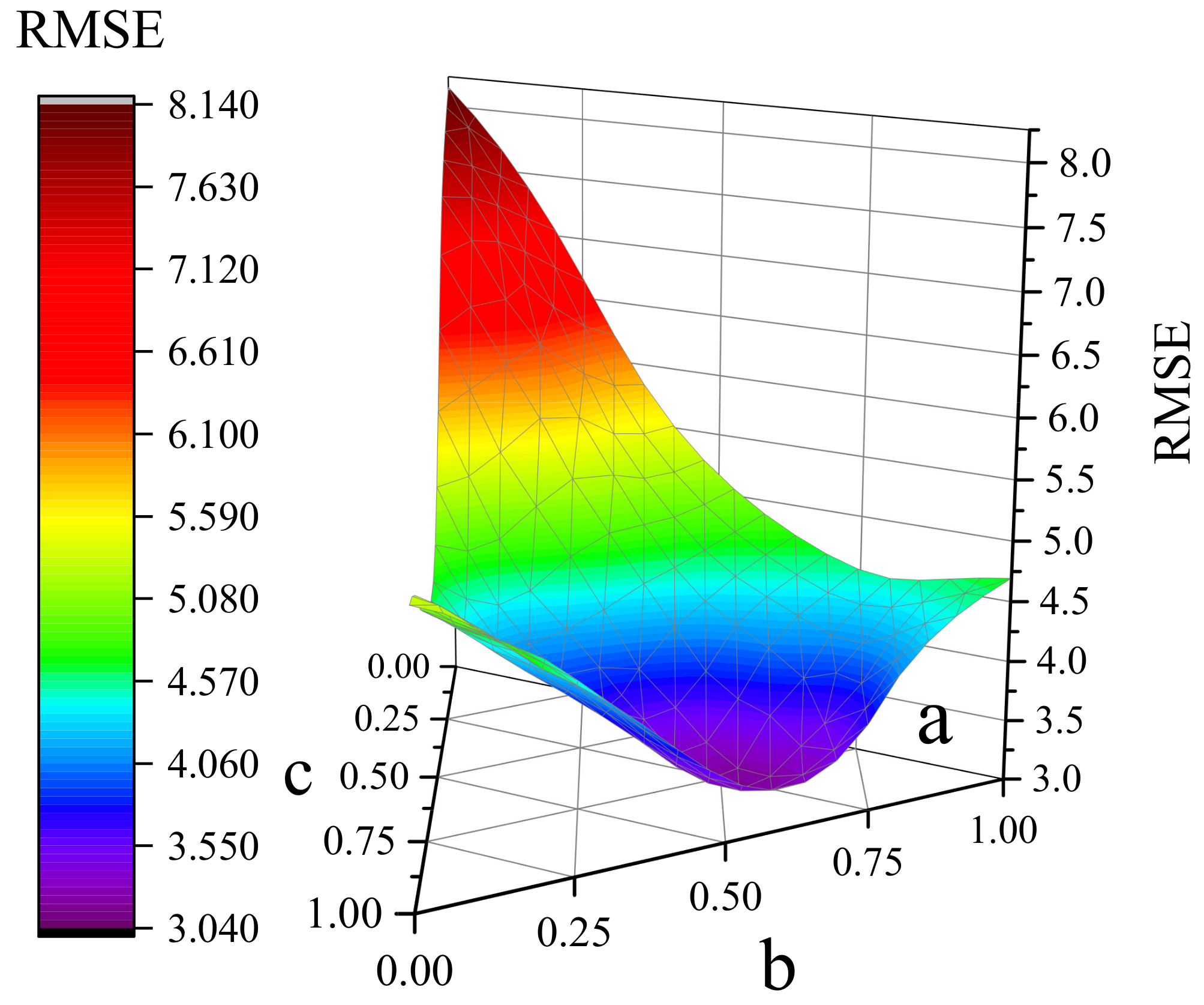
Figure 6 and Figure 7 show the evaluation metrics for the three generators with different weights (a, b, and c respectively represent the output weights of generators $G_1$, $G_2$, and $G_3$). The optimal RMSE, MAE, and R${}^2$ values are obtained when $a=0.2$, $b=0.5$, and $c=0.3$ (i.e., $G_1$ weight is 0.2, $G_2$ weight is 0.5, and $G_3$ weight is 0.3), the weight ratio of $G_2$ is higher than that $G_1$ and $G_3$. The weight of b is increased to determine if this improves the imputation performance. However, the imputation performance does not increase but decreases when $b=0.7$. Thus, increasing the weight ratio of the $G_2$ generator does not improve the model’s performance. In other words, the three generators that receive the vector in flow matrices of the same flow tensor are unfolded in different modes as the input data. Since the internal elements of the different matrix sets after unfolding have different degrees of correlation, each generator is used for each flow matrix. Setting an appropriate weight optimizes the imputation performance.

We conduct extensive experiments by adjusting different values of the respective weights of the three generators to test the imputation performance changes. Figure 8 shows the value changes of RMSE when the weight changes of ternary variables a, b, and c. When a, b, and c are respectively close to the optimal weight value, the RMSE will reach the optimal value.

4.4. Comparison of Different Models

Table 3. Imputation performance of different algorithms.

Method/Indicator	RMSE	MAE	R${}^2$
Matrix-Complete	5.867 ± 0.2204	2.505 ± 0.0469	0.682 ± 0.0183
MICE	5.006 ± 0.1959	1.992 ± 0.0403	0.731 ± 0.0156
CP	4.741 ± 0.2405	2.025 ± 0.0936	0.724 ± 0.0060
missForest	3.763 ± 0.1013	1.759 ± 0.0222	0.882 ± 0.0030
GAIN	3.429 ± 0.1138	1.353 ± 0.0865	0.913 ± 0.0052
ST-GAIN	3.041 ± 0.0464	1.191 ± 0.0435	0.953 ± 0.0018

lists the imputation performances of the ST-GAIN model and five baseline algorithms: CP [33], GAIN [31], Matrix-Complete [5], MICE [6], and missForest [7]. The input data to the GAIN, Matrix-Complete, MICE, and missForest algorithms are the matrix obtained from the horizontal combination of the hourly flow matrix in the study area (equivalent to the matrix unfolded from mode-s of the tensor $\mathcal{N}$). As can be seen from Table 3, the ST-GAIN model has the lowest RMSE and MAE and the highest R${}^2$ value among all models, indicating that the proposed method outperforms the baseline methods for imputation of the traffic dataset with 20% missing values.

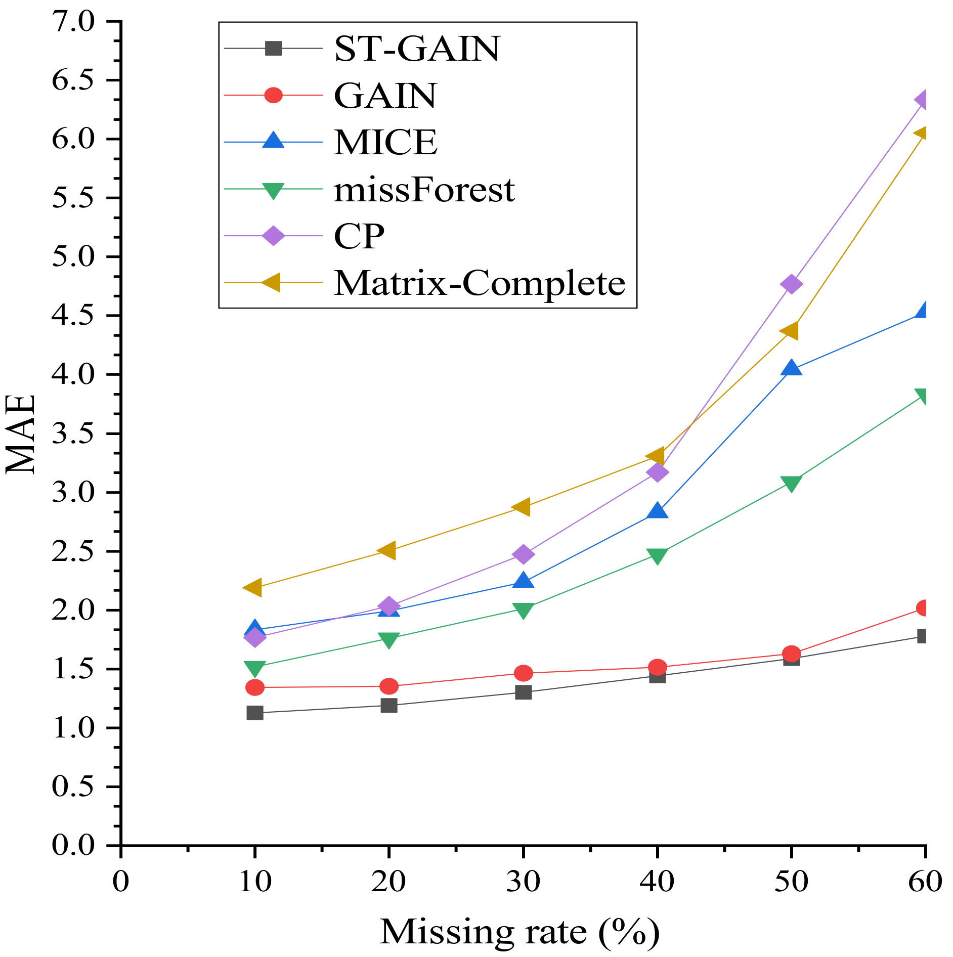
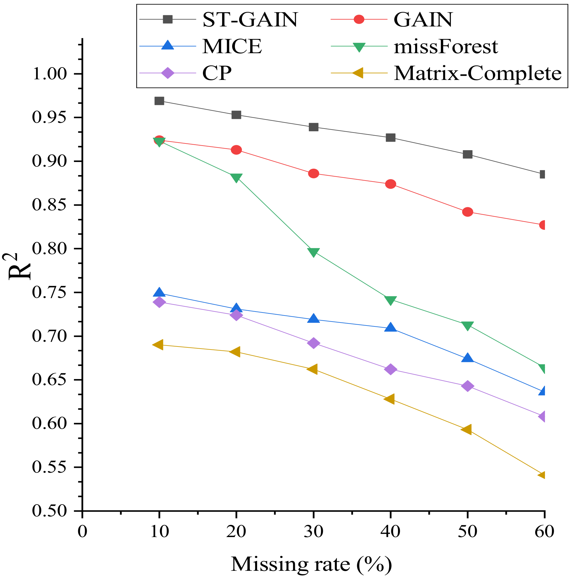
Figure 9, Figure 10 and Figure 11 show the changes of the evaluation metrics (RMSE, MAE, and $R^2$) for the five baseline methods and the ST-GAIN network for different miss rates (10%, 20%, 30%, 40%, 50%, and 60%). The performances of all algorithms decrease as the miss rate increases. ST-GAIN consistently outperforms the other baseline methods in the entire miss rate range, indicating the proposed model’s high robustness and relatively stable imputation performance, especially at a higher miss rate.

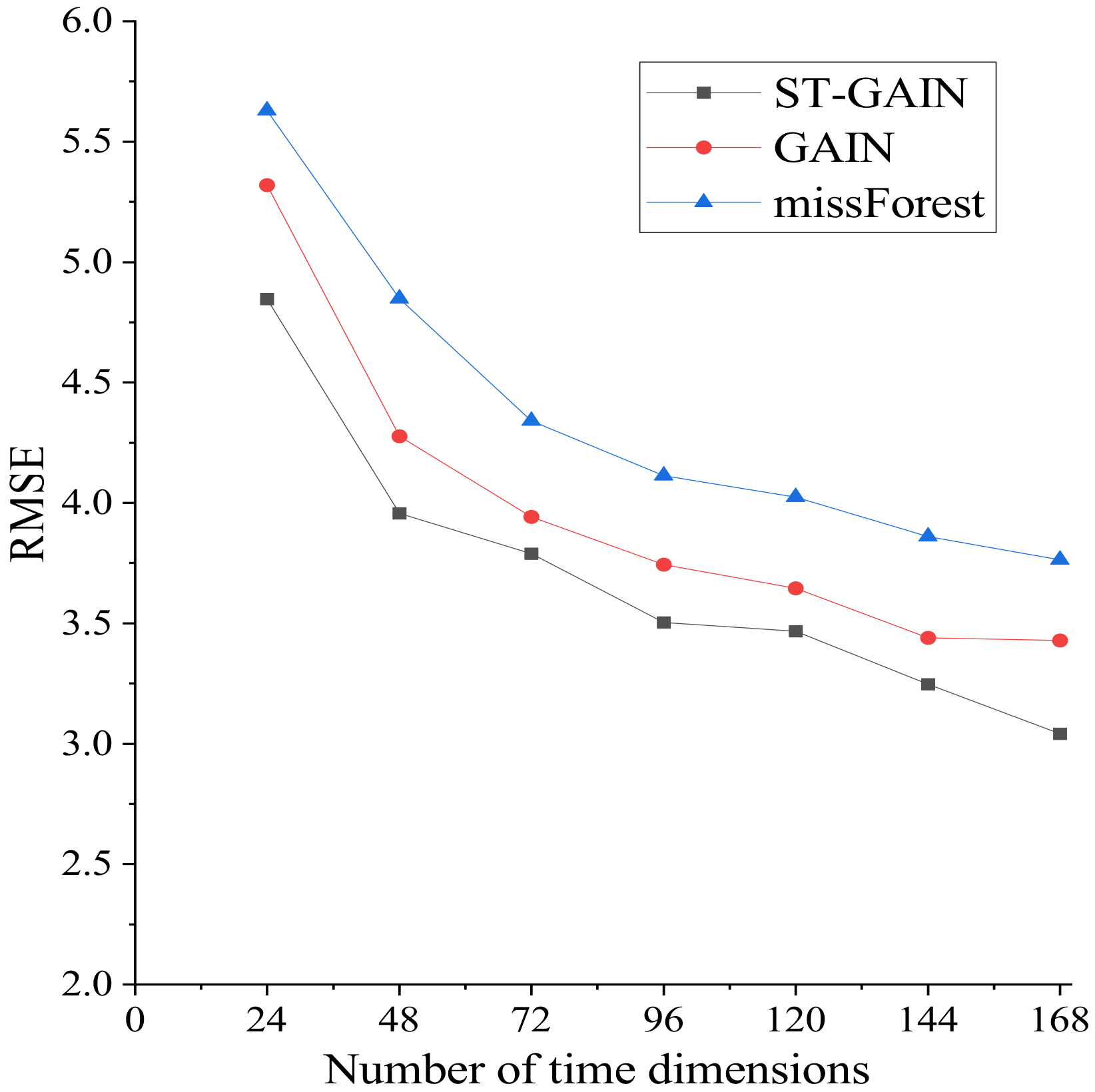
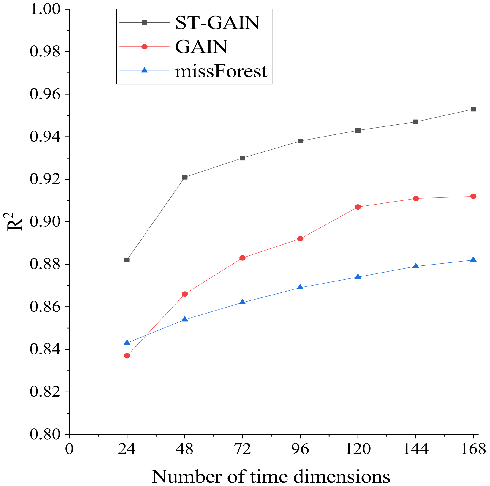
To better understand ST-GAIN, we conduct the following experiments in which we vary the number of temporal dimensions. Figure 12, Figure 13 and Figure 14 show the changes in the evaluation metrics when the temporal dimensions s of our input flow tensor $\mathcal{N}$ is different, which indicates that the constructed tensor $\mathcal{N}$ has different time dimensions (continuous 24, 48, 72, 96, 120, 144, 168 time periods). The figures show that ST-GAIN is also robust to the number of temporal dimensions by comparing to the two most competitive benchmarks (GAIN and missForest). With the increase in the set temporal dimensions in the experiment, the improvement of ST-GAIN is significantly higher than the other two benchmarks.

5. Discussion and Conclusions

This paper proposed the novel ST-GAIN model based on the GAIN network to impute missing elements in spatio-temporal traffic passenger flows data, which typically has random missing values. The method transforms the traffic passenger flows data into a third-order flow tensor and unfolds it into three flow matrices using different modes. Three generators are used to observe and learn the vector components in different matrices, and each generates new vectors to form a flow matrix. The output weight of each generator is determined separately to obtain the generated data after combining the three generators to improve the correlation of the traffic passenger flows data in the spatio-temporal dimensions. We used PCC to define a correlation loss term as part of the generator loss to ensure that the data obtained from the generator are similar to the real data. The experimental results verified that the ST-GAIN model outperformed five baseline imputation methods for filling in missing values using the flow tensor.

In some real scenes, by extracting the three attributes of time, longitude, and latitude of traffic data, and dividing the real geography into grids, the traffic flow matrix information of each time domain in the region can be constructed. The traffic flow information of each time period in a specific range can be obtained without the real traffic network structure information, and it is easier to know the traffic situation of each sub-region in the real geographical region. Moreover, when the traffic data in some partitions cannot be obtained or the data are missing due to the failure of collectors in some partitions, the model ST-GAIN can effectively impute the missing data so that the traffic data with improved quality can be used for the next analysis and utilization.

In future research, we can improve and verify the model’s imputation performance in various ways. Firstly, the traffic flow data exhibit spatio-temporal correlation and were closely related to the quantity and type of points of interest in the city. Future studies can focus on improving the imputation performance of the proposed model by fusing the urban point of interest data with the traffic flow data in the grid and extracting the features. Secondly, this paper only considered the imputation performance of traffic flow data under random missing scenarios. However, in real scenarios, there are various missing patterns in the data. The general adaptability of the ST-GAIN model to various missing data scenarios can be explored and improved in the future. Lastly, the grid size can be changed to verify the performance change of the ST-GIAN model and how to convert the traffic flows under the underlying road network for spatial correlation as input to verify the model.

References

- Zhang, N.; Chen, H.; Chen, X.; Chen, J. Forecasting public transit use by crowdsensing and semantic trajectory mining: Case studies. ISPRS Int. J. Geo-Inf. 2016, 5, 180. [Google Scholar] [CrossRef] [Green Version]
- Chen, Y.; Yuan, P.; Qiu, M.; Pi, D. An indoor trajectory frequent pattern mining algorithm based on vague grid sequence. Expert Syst. Appl. 2019, 118, 614–624. [Google Scholar] [CrossRef]
- Little, R.J.A.; Rubin, D.B. Statistical Analysis with Missing Data; John Wiley Sons: Hoboken, NJ, USA, 2019; Volume 793. [Google Scholar]
- Jadhav, A.; Pramod, D.; Ramanathan, K. Comparison of performance of data imputation methods for numeric dataset. Appl. Artif. Intell. 2019, 33, 913–933. [Google Scholar] [CrossRef]
- Mazumder, R.; Hastie, T.; Tibshirani, R. Spectral regularization algorithms for learning large incomplete matrices. J. Mach. Learn. Res. 2010, 11, 2287–2322. [Google Scholar] [PubMed]
- Royston, P.; White, I.R. Multiple imputation by chained equations (MICE): Implementation in Stata. J. Stat. Softw. 2011, 45, 1–20. [Google Scholar] [CrossRef] [Green Version]
- Stekhoven, D.J.; Bühlmann, P. MissForest—Non-parametric missing value imputation for mixed-type data. Bioinformatics 2012, 28, 112–118. [Google Scholar] [CrossRef] [Green Version]
- Shi, F.; Zhang, D.; Chen, J.; Karimi, H.R. Missing value estimation for microarray data by Bayesian principal component analysis and iterative local least squares. Math. Probl. Eng. 2013, 2013, 162938. [Google Scholar] [CrossRef]
- Shang, Q.; Yang, Z.; Gao, S.; Tan, D. An imputation method for missing traffic data based on FCM optimized by PSO-SVR. J. Adv. Transp. 2018, 2018, 2935248. [Google Scholar] [CrossRef]
- Tang, J.; Zhang, G.; Wang, Y.; Wang, H.; Liu, F. A hybrid approach to integrate fuzzy C-means based imputation method with genetic algorithm for missing traffic volume data estimation. Transp. Res. Part C Emerg. Technol. 2015, 51, 29–40. [Google Scholar] [CrossRef]
- Meng, H.; Chen, S. A comparative analysis of data imputation methods for missing traffic flow data. J. Transp. Inf. Saf. 2018, 36, 61–67. [Google Scholar]
- Zhang, A.; Song, S.; Sun, Y.; Wang, J. Learning individual models for imputation. In Proceedings of the 2019 IEEE 35th International Conference on Data Engineering (ICDE), Macao, China, 8–11 April 2019; pp. 160–171. [Google Scholar]
- Tang, J.; Zhang, X.; Yu, T.; Liu, F. Missing traffic data imputation considering approximate intervals: A hybrid structure integrating adaptive network-based inference and fuzzy rough set. Phys. A Stat. Mech. Appl. 2021, 573, 125776. [Google Scholar] [CrossRef]
- Li, L.; Zhang, J.; Wang, Y.; Ran, B. Missing value imputation for traffic-related time series data based on a multi-view learning method. IEEE Trans. Intell. Transp. Syst. 2018, 20, 2933–2943. [Google Scholar] [CrossRef]
- Luo, Y.; Cai, X.; Zhang, Y.; Xu, J. Multivariate time series imputation with generative adversarial networks. Adv. Neural Inf. Process. Syst. 2018, 31, 1603–1614. [Google Scholar]
- Wang, L.; Li, M.; Yan, J.Q. Urban traffic flow data recovery method based on generative adversarial network. J. Sci. J. Transp. Syst. Eng. Inf. Technol. 2018, 18, 63–71. [Google Scholar]
- Luo, Y.; Zhang, Y.; Cai, X.; Yuan, X. E2gan: End-to-end generative adversarial network for multivariate time series imputation. In Proceedings of the 28th International Joint Conference on Artificial Intelligence, Macao, China, 10–16 August 2019; pp. 3094–3100. [Google Scholar]
- Yang, B.; Kang, Y.; Yuan, Y.; Huang, X.; Li, H. ST-LBAGAN: Spatio-temporal learnable bidirectional attention generative adversarial networks for missing traffic data imputation. Knowl.-Based Syst. 2021, 215, 106705. [Google Scholar] [CrossRef]
- Tan, H.; Yang, Z.; Feng, G.; Wang, W.; Ran, B. Correlation analysis for tensor-based traffic data imputation method. Procedia-Soc. Behav. Sci. 2013, 96, 2611–2620. [Google Scholar] [CrossRef] [Green Version]
- Yan, J.; Li, H.; Bai, Y.; Lin, Y. Spatial—Temporal Traffic Flow Data Restoration and Prediction Method Based on the Tensor Decomposition. Appl. Sci. 2021, 11, 9220. [Google Scholar] [CrossRef]
- Chen, X.; Lei, M.; Saunier, N.; Sun, L. Low-rank autoregressive tensor completion for spatiotemporal traffic data imputation. IEEE Trans. Intell. Transp. Syst. 2022, 23, 12301–12310. [Google Scholar] [CrossRef]
- Zhang, Y.F.; Thorburn, P.J.; Xiang, W.; Fitch, P. SSIM—A deep learning approach for recovering missing time series sensor data. IEEE Internet Things J. 2019, 6, 6618–6628. [Google Scholar] [CrossRef]
- Wang, X.; Ma, Y.; Huang, S.; Xu, Y. Data Imputation for Detected Traffic Volume of Freeway Using Regression of Multilayer Perceptron. J. Adv. Transp. 2022, 2022, 4840021. [Google Scholar] [CrossRef]
- Che, Z.; Purushotham, S.; Cho, K.; Sontag, D.; Liu, Y. Recurrent neural networks for multivariate time series with missing values. Sci. Rep. 2018, 8, 6085. [Google Scholar] [CrossRef] [PubMed] [Green Version]
- Cao, W.; Wang, D.; Li, J.; Zhou, H.; Li, L.; Li, Y.B. Bidirectional recurrent imputation for time series. arXiv 2018, arXiv:1805.10572. [Google Scholar]
- Zhao, Q.; Zhang, L.; Cichocki, A. Bayesian CP factorization of incomplete tensors with automatic rank determination. IEEE Trans. Pattern Anal. Mach. Intell. 2015, 37, 1751–1763. [Google Scholar] [CrossRef] [PubMed] [Green Version]
- Zhou, W.; Zheng, H.; Feng, X.; Lin, D. A multi-source based coupled tensors completion algorithm for incomplete traffic data imputation. In Proceedings of the 2019 11th International Conference on Wireless Communications and Signal Processing (WCSP), Xi’an, China, 23–25 October 2019; pp. 1–6. [Google Scholar]
- Li, Q.; Tan, H.; Wu, Y.; Ye, L.; Ding, F. Traffic flow prediction with missing data imputed by tensor completion methods. IEEE Access 2020, 8, 63188–63201. [Google Scholar] [CrossRef]
- Cai, L.; Wang, H.; Sha, C.; Jiang, F.; Zhang, Y.; Zhou, W. The mining of urban hotspots based on multi-source location data fusion. IEEE Trans. Knowl. Data Eng. 2023, 35, 2061–2077. [Google Scholar] [CrossRef]
- Duan, Y.; Lv, Y.; Kang, W. A deep learning based approach for traffic data imputation. In Proceedings of the 17th International IEEE Conference on Intelligent Transportation Systems (ITSC), Qingdao, China, 8–11 October 2014; pp. 912–917. [Google Scholar]
- Yoon, J.; Jordon, J.; Schaar, M. Gain: Missing data imputation using generative adversarial nets. In Proceedings of the International Conference on Machine Learning, Stockholm, Sweden, 10–15 July 2018; pp. 5689–5698. [Google Scholar]
- Goodfellow, I.; Pouget-Abadie, J.; Mirza, M. Generative adversarial nets. Commun. ACM 2020, 63, 139–144. [Google Scholar] [CrossRef]
- Wu, Y.; Tan, H.; Li, Y.; Zhang, J.; Chen, X. A fused CP factorization method for incomplete tensors. IEEE Trans. Neural Netw. Learn. Syst. 2018, 30, 751–764. [Google Scholar] [CrossRef]
- Cho, K.; Van Merriënboer, B.; Gulcehre, C.; Bahdanau, D.; Bougares, F.; Schwenk, H.; Bengio, Y. Learning phrase representations using RNN encoder-decoder for statistical machine translation. arXiv 2014, arXiv:1406.1078. [Google Scholar]
- Chen, Y.; Lv, Y.; Wang, F.Y. Traffic flow imputation using parallel data and generative adversarial networks. IEEE Trans. Intell. Transp. Syst. 2019, 21, 1624–1630. [Google Scholar] [CrossRef]
- Wang, P.; Zhang, T.; Zheng, Y.; Hu, T. A multi-view bidirectional spatiotemporal graph network for urban traffic flow imputation. Int. J. Geogr. Inf. Sci. 2022, 36, 1231–1257. [Google Scholar] [CrossRef]
- Wang, P.; Hu, T.; Gao, F.; Wu, R.; Guo, W.; Zhu, X. A hybrid data-driven framework for spatiotemporal traffic flow data imputation. IEEE Internet Things J. 2022, 9, 16343–16352. [Google Scholar] [CrossRef]
- Jin, L.; Li, Y. Analysis of Several Correlation Coefficients and Their Implementation in R Language. Stat. Inf. Forum 2019, 34, 3–11. [Google Scholar]
- Yap, B.W.; Sim, C.H. Comparisons of various types of normality tests. J. Stat. Comput. Simul. 2011, 81, 2141–2155. [Google Scholar] [CrossRef]
Figure 1.
Missing characteristics of regional traffic flow data. (Black squares indicate missing data.) (a) The flow is missing randomly within the area; (b) missing flow in the continuous time domain within the area.
Figure 2.
Distribution of pick-up and drop-off points in parts of the area. (Blue dots are pick-up points, and red dots are drop-off points).
Figure 3.
Traffic passenger flows at different times of the day in adjacent grids.
Figure 4.
Traffic passenger flows in grid 634 at different times on 5 working days.
Figure 5.
The architecture of ST-GAIN model.
Figure 6.
RMSE and MAE values for different generator weights.
Figure 7.
R values for different generators weights.
Figure 8.
RMSE under different values of ternary variables. (a–c) respectively represent the output weights of generators G1, G2, and G3.
Figure 9.
MAE for different miss rates.
Figure 10.
RMSE for different miss rates.
Figure 11.
R for different miss rates.
Figure 12.
RMSE for different time dimensions.
Figure 13.
MAE for different time dimensions.
Figure 14.
R for different time dimensions.