A Geographic Information Systems (GIS)-Based Approach to Derivative Map Production and Visualizing Bedrock Topography within the Town of Rutland, Vermont, USA

Abstract
:1. Introduction
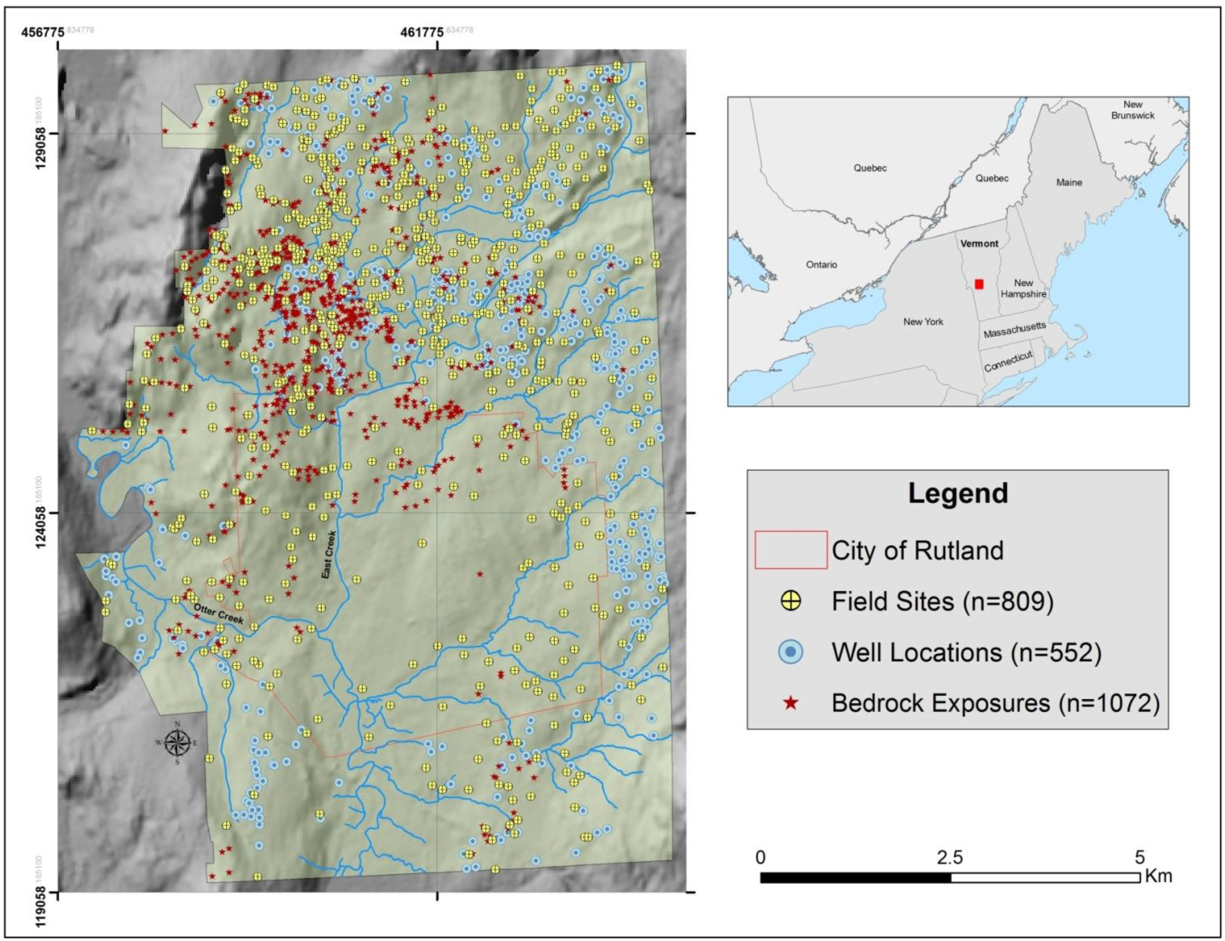
2. Study Area

3. Methodology


| Cross Validation Prediction Error Results—Kriging | ||||
|---|---|---|---|---|
| Variogram Type | Mean Prediction Error | RMS Error | Average Standard Error | RMS Standardized |
| Circular | 0.02 | 36.83 | 26.37 | 1.38 |
| Spherical | 0.02 | 36.91 | 25.66 | 1.42 |
| Tetrapsherical | 0.02 | 37.01 | 24.95 | 1.47 |
| Pentaspherical | 0.02 | 37.11 | 24.24 | 1.52 |
| Exponential | −0.01 | 42.21 | 14.15 | 3.61 |
| Gaussian | −0.05 | 36.74 | 33.11 | 1.11 |
| Rational Quadratic | 0.05 | 36.55 | 30.10 | 1.20 |
| Hole Effect | −0.05 | 36.72 | 33.23 | 1.10 |
| K-Bessel | −0.05 | 36.73 | 33.18 | 1.10 |
| J-Bessel | −0.04 | 36.72 | 33.28 | 1.09 |
| Stable | −0.05 | 36.74 | 33.13 | 1.11 |
| Validation Prediction Error Results – Kriging | ||||
|---|---|---|---|---|
| Variogram Type | Mean Prediction Error | RMS Error | Average Standard Error | RMS Standardized |
| Circular | −0.24 | 28.67 | 26.46 | 1.06 |
| Spherical | −0.31 | 28.61 | 25.76 | 1.11 |
| Tetrapsherical | −0.32 | 28.56 | 25.07 | 1.11 |
| Pentaspherical | −0.34 | 28.52 | 24.36 | 1.14 |
| Exponential | −0.90 | 29.76 | 14.64 | 2.75 |
| Gaussian | 0.27 | 30.92 | 33.12 | 0.93 |
| Rational Quadratic | −0.28 | 29.47 | 30.13 | 0.97 |
| Hole Effect | 0.23 | 30.81 | 33.24 | 0.92 |
| K-Bessel | 0.24 | 30.83 | 33.19 | 0.92 |
| J-Bessel | 0.22 | 30.78 | 33.29 | 0.91 |
| Stable | 0.26 | 30.90 | 33.14 | 0.93 |
4. Results and Discussion
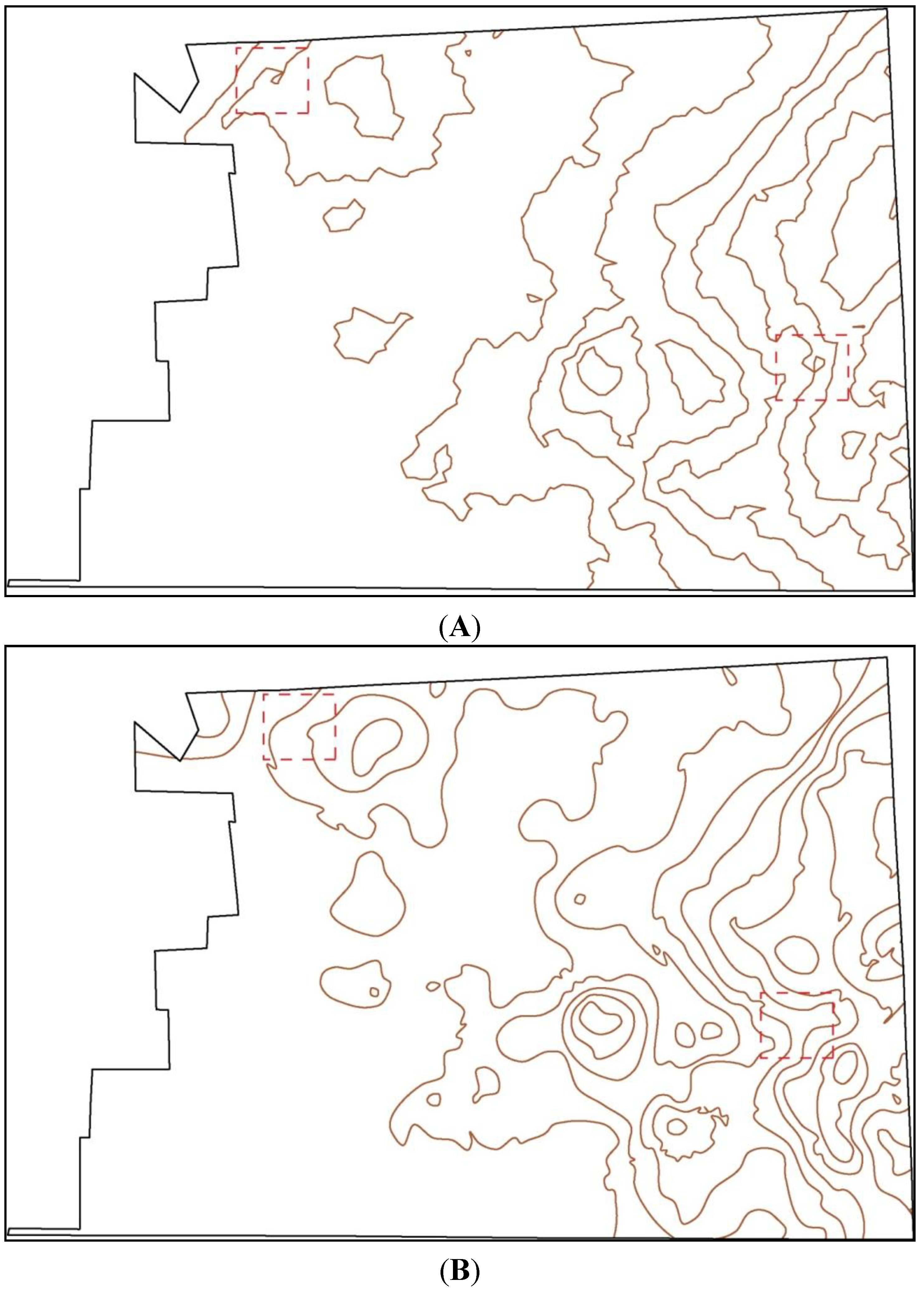
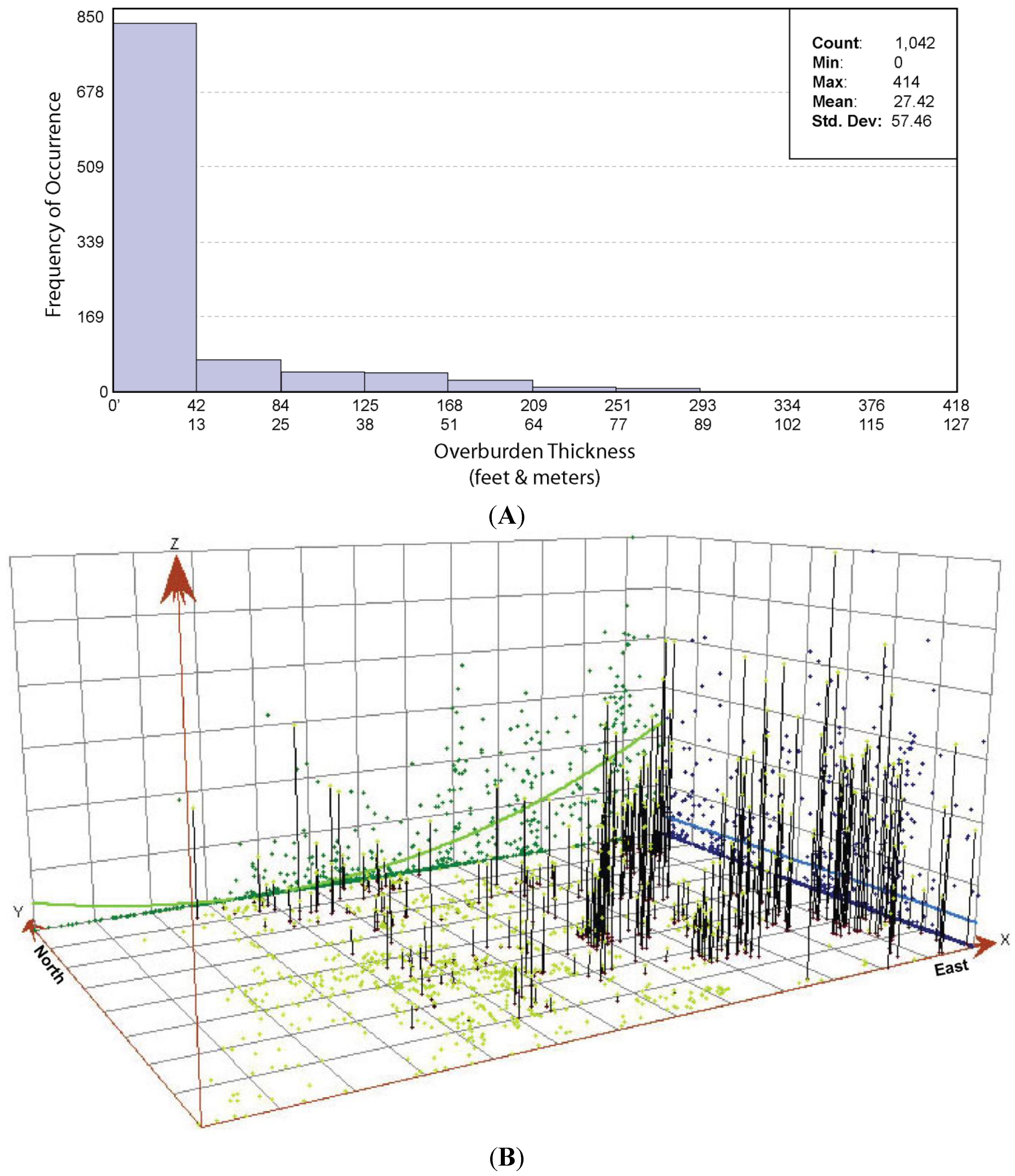
4.1. Isopach Map
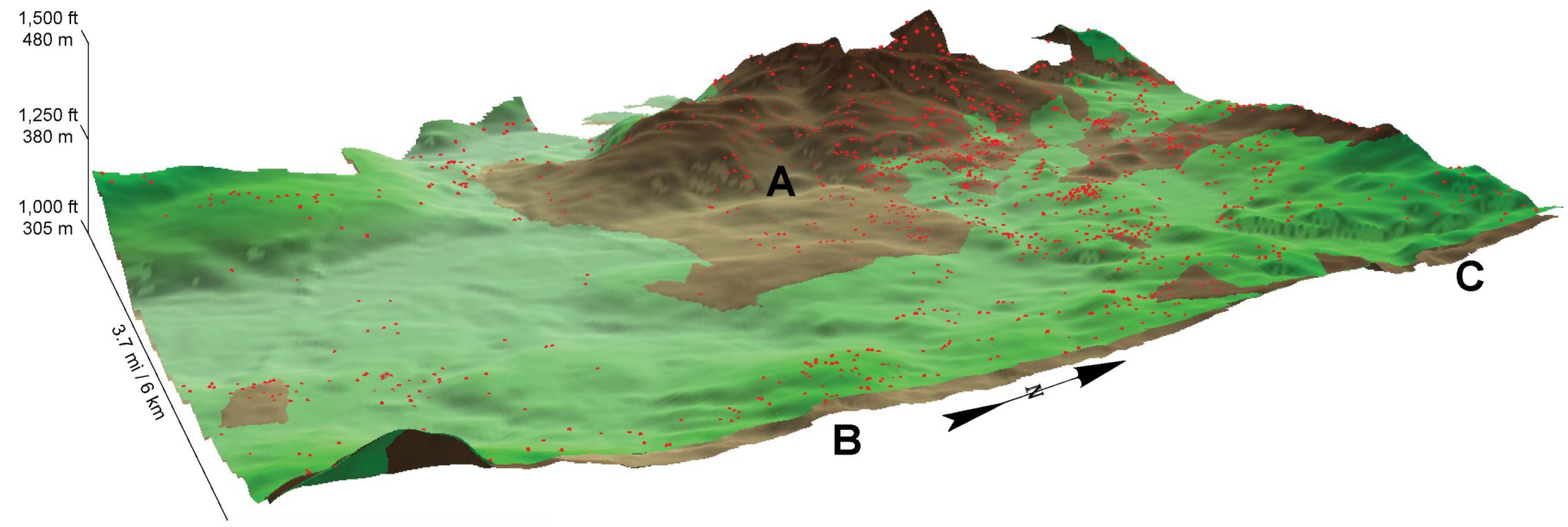
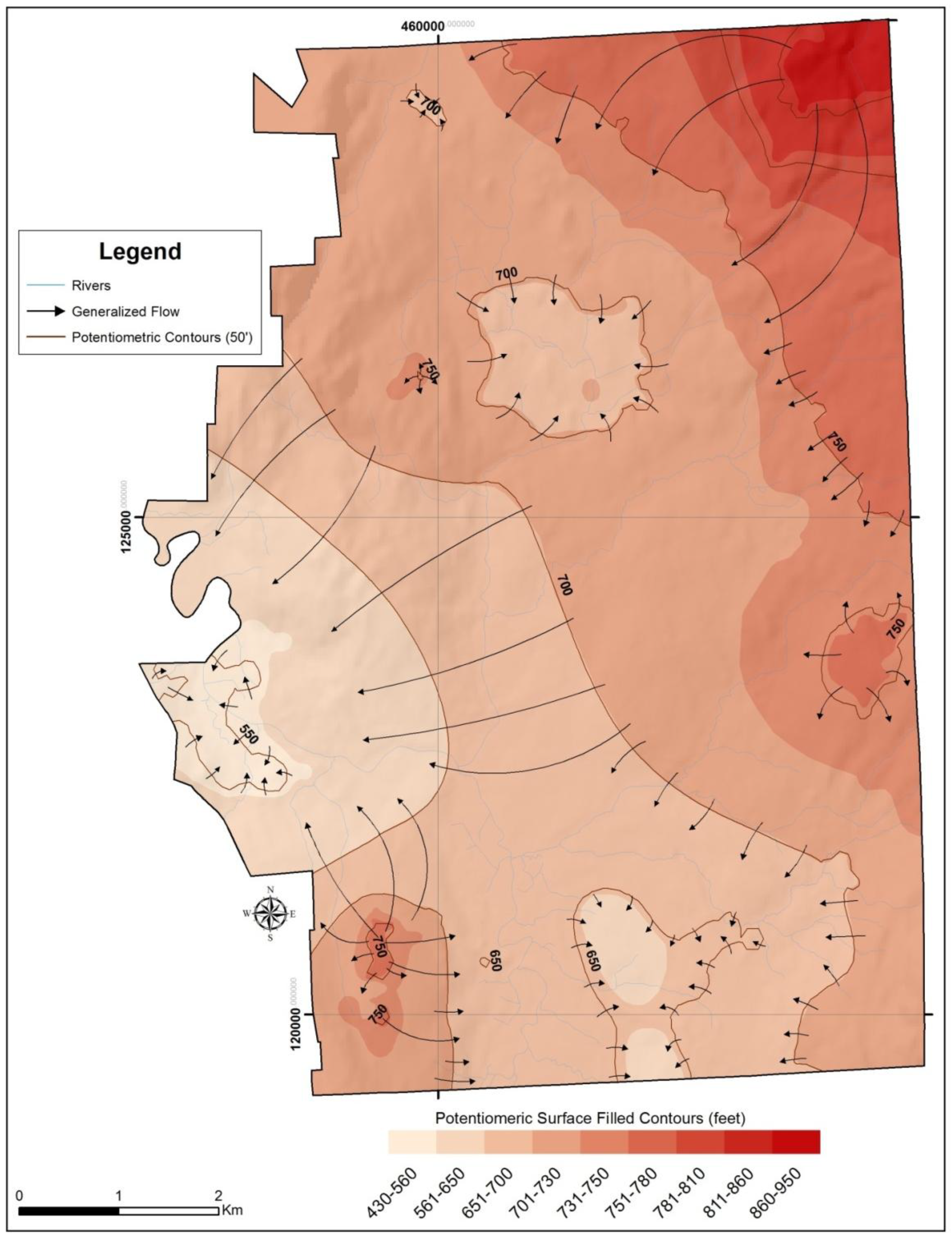
4.2. Potentiometric Surface


5. Discussion
6. Conclusion
Acknowledgments
Conflicts of Interest
References and Notes
- Bernknopf, R.L.; Brookshire, D.S.; Soller, D.R.; McKee, M.J.; Sutter, J.F.; Matti, J.C.; Campbell, R.H. Societal Value of Geologic Maps. Available online: http://pubs.usgs.gov/circ/1993/1111/report.pdf (accessed on 1 December 2013).
- Bhagwat, S.B.; Ipe, V.C. The Economic Benefits of Detailed Geologic Mapping to Kentucky. Available online: https://www.ideals.illinois.edu/bitstream/handle/2142/45219/economicbenefits03bhag.pdf (accessed on 1 December 2013).
- Johnston, K.M.; Ver Hoef, J.; Krivoruchko, K.; Lucas, N. Using the Geostatistical Analyst; ESRI Press: Redlands, CA, USA, 2004; p. 306. [Google Scholar]
- Desbarats, A.J.; Logan, C.E.; Hinton, M.J.; Sharpe, D.R. On the kriging of water table elevations using collateral information from a digital elevation model. J. Hydrol. 2002, 255, 25–38. [Google Scholar] [CrossRef]
- Gao, C.; Shirota, J.; Kelly, R.I.; Brunton, F.R.; van Haaften, S. Bedrock topography and Overburden Thickness Mapping, Southern Ontario. Available online: http://www.geologyontario.mndm.gov.on.ca/mndmfiles/pub/data/imaging/MRD207/MRD207BedrockTopMapping.pdf (accessed on 1 December 2013).
- Kassenaar, J.D.C.; Wexler, E.J. Groundwater Modeling of the Oak Ridges Moraine Area. Available online: http://www.ypdt-camc.ca/Publications/CAMCYPDTReports/tabid/221/Default.aspx (accessed on 1 December 2013).
- Logan, C.; Russell, H.A.J.; Sharpe, D.R. The Role of GIS and Expert Knowledge in 3-D Modeling Oak Ridges Moraine, Southern Ontario. Available online: http://data.gc.ca/data/en/dataset/bb5801cd-f42c-5fe7-af2d-f93361d776af (accessed on 1 December 2013).
- Paulen, R.C.; McClenaghan, M.B.; Harris, J.R. Bedrock Topography and Drift Thickness Models from the Timmins Area, Northeastern Ontario: An application of GIS to the Timmins Overburden Drillhole Database. In An Application of GIS to the Timmins Overburden Drillhole Database; Geological Association of Canada: St. John’s, Canada, 2006; pp. 413–444. [Google Scholar]
- Spahr, P.N.; Jones, A.W.J.; Barret, K.A.; Angle, M.P.; Raab, J.M. Using GIS to Create and Analyze Potentiometric-Surface Maps; US Geological Survey Open-File Report 2007–1285; US Geological Survey: Reston, VA, USA, 2007.
- Locke, R.A.; Meyers, S.C. Kane County Water Resources Investigations: Final Report on Shallow Aquifer Potentiometric Surface Mapping; Contract Report 2007-6; Illinois State Water Survey: Champaign, IL, USA, 2007. [Google Scholar]
- Venteris, E.R. 3D modeling of glacial stratigraphy using public water well data, geologic interpretation and geostatistics. Geosphere 2007, 3, 456–468. [Google Scholar] [CrossRef]
- Nageswara Rao, K.; Bhaskara, Ch.U.; Venkateswara Rao, T. Estimation of sediment volume through geophysical and GIS analyses—A case study of the red sand deposit along Visakhapatnam Coast. J. Indian Geophys. Union 2008, 12, 23–30. [Google Scholar]
- Strassberg, G.; Jones, N.L.; Lemon, A. ArcHydro Groundwater Data Model and Tools: Overview and Use Cases. Available online: http://www.acquesotterranee.it/en/rivista/aquamundi/articoli/arc-hydro-groundwater-data-model-and-tools-overview-and-use-cases (accessed on 6 January 2014).
- Berg, R.C.; Mathers, S.J.; Kessler, H.; Keefer, D.A. Synopsis of current three-dimensional geological mapping and modeling in geological survey organizations. Ill. State Geol. Surv. Circ. 2011, 578, 92. [Google Scholar]
- Samui, P.; Sitharam, T.G. Application of geostatistical methods for estimating spatial variability of rock depth. Engineering 2011, 3, 886–894. [Google Scholar] [CrossRef]
- Trabelsi, F.; Tarhouni, J.; Mammou, A.B.; Ranieri, G. GIS-based subsurface databases and 3-D geological modeling as a tool for the set up of a hydrogeological framework: Nabeul-Hammamet coastal aquifer case study (Northern Tunisia). Environ. Earth Sci. 2011, 70, 2087–2105. [Google Scholar]
- Rao, T.V.; Naik, D.R.; Rao, V.V.; Swamy, C.J. Estimation of aquifer volume using geophysical and GPS studies for a part of Mehadrigedda Reservoir catchment, Visakhaptnam, India—A 3-dimensional modelling approach using GIS. Int. J. Civil, Struct. Environ. Infrastruct. Eng. 2013, 3, 155–164. [Google Scholar]
- Ratcliffe, N.M. Digital and Preliminary Bedrock Geologic Map of the Rutland Quadrangle, Vermont; USGS Open-File Report 98-121; US Geological Survey: Reston, VA, USA, 1998.
- Nicholson, S.W.; Dicken, C.L.; Horton, J.D.; Foose, M.P.; Mueller, J.A.L.; Hon, R. Preliminary Integrated Geologic Map Databse for the United States: Connecticut, Maine, Massachusetts, New Hampshire, New Jersey, Rhode Island, and Vermont; US Geological Survey Open-File Report 2006-1272; US Geological Survey: Reston, VA, USA, 2006.
- Van Hoesen, J.G. Surficial Geologic Map of Rutland, Vermont; Vermont Geological Survey Open File Report VG09-7; US Geological Survey: Reston, VA, USA, 2009.
- Ratcliffe, N.M. Preliminary Bedrock Geologic Map of the Chittenden Quadrangle, Rutland County, Vermont; US Geological Survey Open-File Report 97-703; US Geological Survey: Reston, VA, USA, 1997.
- Bajjali, W. Model the effect of four artificial recharge dams on the quality of groundwater using geostatistical methods in GIS environment, Oman. J. Spatial Hydrol. 2005, 5, 1–15. [Google Scholar]
- Gold, C.M. Drill-hole Data Validation for Subsurface Stratigraphic Modeling. In Computer Mapping of Natural Resources and the Environment; Harvard University, Laboratory for Computer Graphics and Spatial Analysis: Cambridge, MA, US, 1979; pp. 52–58. [Google Scholar]
- Chang, K. Introduction to Geographic Information Systems; McGraw Hill Publisher: New York, NY, USA, 2004. [Google Scholar]
- Yang, X.; Hodler, T. Visual and statistical comparisons of surface modeling techniques for point-based environmental data. Cartogr. Geogra. Inf. Syst. 2000, 27, 165–175. [Google Scholar] [CrossRef]
- Hiscock, K. Hydrogeology: Principles and Practice, 1st ed.; Wiley-Blackwell: Oxford, UK, 2005. [Google Scholar]
- Ely, M.G. The differential susceptibility of topographic map interpretation to influence from training. Appl. Cogn. Psychol. 1993, 7, 23–42. [Google Scholar] [CrossRef]
- Schofield, N.J.; Kirby, J.R. Position location on topographical maps: Effects of task factors, training and strategies. Cogn. Instr. 1994, 12, 35–60. [Google Scholar] [CrossRef]
- Gerson, H.B.; Sorby, S.A.; Wysocki, A.; Baartmans, B.J. The development and assessment of multimedia software for improving 3D spatial visualization skills. Comput. Appl. Eng. Educ. 2001, 9, 105–113. [Google Scholar] [CrossRef]
- Uttal, D.H. Seeing the big picture: Map use and the development of spatial cognition. Dev. Sci. 2000, 3, 247–286. [Google Scholar]
- Libarkin, J.; Brick, C. Research methodologies in science education. J. Geosci. Educ. 2002, 50, 449–455. [Google Scholar]
- Hunt, B.; Banada, N.; Smith, B.A. Three-dimensional geological model of the Barton Springs segment of Edwards Aquifer, Central Texas. Gulf Coast Assoc. Geol. Soc. Trans. 2010, 60, 355–367. [Google Scholar]
- House, P.K.; Clark, R.; Kopera, J. Overcoming the Momentum of Anachronism: American Geologic Mapping in a Twenty-first Century World. In Rethinking the Fabric of Geology; Baker, V.R., Ed.; The Geological Society of America: Boulder, CO, USA, 2013; pp. 103–125. [Google Scholar]
© 2014 by the authors; licensee MDPI, Basel, Switzerland. This article is an open access article distributed under the terms and conditions of the Creative Commons Attribution license (http://creativecommons.org/licenses/by/3.0/).
Share and Cite
Van Hoesen, J.G. A Geographic Information Systems (GIS)-Based Approach to Derivative Map Production and Visualizing Bedrock Topography within the Town of Rutland, Vermont, USA. ISPRS Int. J. Geo-Inf. 2014, 3, 130-142. https://doi.org/10.3390/ijgi3010130
Van Hoesen JG. A Geographic Information Systems (GIS)-Based Approach to Derivative Map Production and Visualizing Bedrock Topography within the Town of Rutland, Vermont, USA. ISPRS International Journal of Geo-Information. 2014; 3(1):130-142. https://doi.org/10.3390/ijgi3010130
Chicago/Turabian StyleVan Hoesen, John G. 2014. "A Geographic Information Systems (GIS)-Based Approach to Derivative Map Production and Visualizing Bedrock Topography within the Town of Rutland, Vermont, USA" ISPRS International Journal of Geo-Information 3, no. 1: 130-142. https://doi.org/10.3390/ijgi3010130