An Automatic Matcher and Linker for Transportation Datasets

Abstract

Multimodality requires the integration of heterogeneous transportation data to construct a broad view of the transportation network. Many new transportation services are emerging while being isolated from previously-existing networks. This leads them to publish their data sources to the web, according to linked data principles, in order to gain visibility. Our interest is to use these data to construct an extended transportation network that links these new services to existing ones. The main problems we tackle in this article fall in the categories of automatic schema matching and data interlinking. We propose an approach that uses web services as mediators to help in automatically detecting geospatial properties and mapping them between two different schemas. On the other hand, we propose a new interlinking approach that enables the user to define rich semantic links between datasets in a flexible and customizable way.

1. Introduction

Multimodality requires the integration of heterogeneous transportation data to construct a broad view of the transportation network. The transportation field is continuously evolving with new services that are growing quickly to take part in passengers’ daily commute or travel, e.g., car pooling (https://www.blablacar.fr/), car sharing (https://www.deways.com/ or https://www.drivy.com/) and bike sharing (https://www.velib.fr). The problem is that these services differ in data representation, and there is no specific standard for them to follow. This results in people manually combining different sub-trips from different sources (websites or applications) in order to create optimized trips that fit their needs. Such a task requires users to be fully aware of the surrounding services in addition to a complex task of finding links between one system and another. This raises the need for integrating multiple transportation data in order to provide a global view of the network. Enabling such a solution for each company requires identifying the nearby services and finding ways to integrate them, which is a repetitive and tedious task, especially when done manually. This limits operators to isolated solutions, which have to understand, translate and integrate every single relevant data source. Even though this task is a complicated one, it becomes even more complex when considering the evolution of the integrated data and the necessity of maintaining them and keeping them up to date. Some approaches have moved into creating a public repository to integrate public transportation data (Google Transit (http://maps.google.com/landing/transit/index.html), Syndicat des transports d’ile-de-France (STIF) (http://www.stif.info)); however, they still do not take into consideration highly-evolving datasets, such as car sharing, bike sharing, car pooling, etc. Such services are highly dynamic and do not always have the notion of a fixed transportation stop.

Our goal is to find a simple way for operators to identify nearby transportation services by providing a connection portal enabling one to identify the connections between one transportation data source to other sources. In this work, we approach this problem from two perspectives. The first one is at the schema level, and it targets the automatic integration of datasets with different schemas. The second one is at the instance level, and it targets the discovery of transportation relations between different entities scattered between the datasets. We propose a homogeneous light-weight representation of transportation connections (transfer points from one stop to another) and the means to discover them in a flexible and customized manner. With this representation, we can link different types of transportation services regardless of the mode or service they offer. All transportation systems need to know is just how to handle these light connections and use them to connect with the outer world, which is much simpler than handling heterogeneous data and maintaining them.

In this article, we tackle two main problems from both fields: automatic schema matching and data interlinking.

1.1. Schema Matching

Automatic schema matching/mapping aims at proposing an automated way of discovering matching rules between datasets. However, the domain of transportation has some specific characteristics that existing approaches cannot handle. Transportation data contain geospatial properties that are represented in various formats and structures. A simple example to be considered is how an address can be modeled in different sources. Figure 1 shows three different representations for the same real-world address.

Figure 1a shows a model that combines the attributes Street1, Street2, Zip-code, City and a Country to represent an address. Figure 1b shows the address as a combination of latitude and longitude values, while the final Figure 1c shows a WKT (http://www.opengeospatial.org/standards/wkt-crs) (well-known text) representation of the same entity.

In order to detect a mapping between different representations, existing approaches use individual or combined matchers that work on schema and/or instance levels using various techniques, e.g., linguistic, constraint-based, data-type based, etc. However, the mathematical-based operators used to define the similarity between relations are not suitable alone to detect the complex relations in transportation data. For instance, there is no way to find out that a combination of street1, street2, zip-code, city and country is the same as a combination of latitude and longitude between two datasets by using only some mathematical functions. This problem raises the question of how we can be able to automatically identify and map different representations of geospatial characteristics between two schemas.

The fact that each transportation dataset may contain different instances is a challenge since we cannot rely on the basic instance matching techniques to know the schema mappings. Moreover, relying only on other properties, such as column names or value types, may not be sufficient by themselves. To tackle this problem, we introduce an instance-based approach to detect geospatial properties for transportation points of transfers by the use of geospatial web services.

1.2. Data Interlinking

Enabling a transportation integration solution requires access to transportation sources, which can be obtained from open data [1,2], which is gaining a great deal of popularity, and numerous transportation operators are using it to publish their data on the web in order to increase their market visibility (http://opendata.paris.fr/page/home/, http://www.strasbourg.eu/ma-situation/professionnel/open-data/donnees/mobilite-transport-open-data, http://www.uitp.org/tags/open-data). Many solutions have benefited from this to provide rich data for smart city applications. They use linked data techniques and data interlinking tools to provide extended information relevant to both transportation and passenger profile queries [3,4]. These techniques address equivalence detection between entities to establish links between data sources. This may help in enriching data about entities. However, this is not always enough in transportation data. Further complex relations are required to reflect the nature of transportation connections. Beyond equivalence or sameAslinks, we are interested in finding connections between transportation data sources based on the geospatial characteristics of the data, which capture the reachability between different transportation networks. Furthermore, using the given tools, we face two main limitations. The first is the restriction to a predefined set of functions for composing linking rules, due to the lack of flexibility of existing systems in defining custom functions. For instance, to calculate information such as the closeness of two transportation points of transfer (bus stop, train station, etc.), we cannot define custom functions to calculate walking distances, driving distances, etc. The user is forced to dig into the code (if available) and modify it directly. The second limitation is the representation of the generated output. Supporting complex relations requires more complex output patterns. As an example, let us suppose that a link is established between two transportation points of transfers. Existing tools can provide the output (BusStop1 nextTo TrainStation132) which does not give information about the occurrence of this relation. They are next to each others, but how close are they, and what are the modes of transportation that we can use, etc.?

This article is structured as follows: In Section 2, we present the background work and related work to both the automatic schema matching and data interlinking domains. Our contributions are then presented in Section 3 and Section 4. Section 3 discusses our automatic schema-matching approach for transportation datasets. Section 4 discusses our flexible and customizable way of generating transportation connections for open data transportation datasets. Later, both approaches are put up to test with a real case scenario represented in Section 5. Finally, we conclude our work and discuss some perspectives in Section 6.

2. State of the Art

2.1. Automatic Schema Matching

Automatic schema matching is one of the approaches to solve schema heterogeneity. It provides the means and the techniques necessary for uniform access to the data.

Based on [5,6,7], a mapping element is a five-uple: $(id,e,e^{\prime },n,R)$ where:

• id is a unique identifier of the given mapping element
• e and e’ are the entities of the first schema/ontology, respectively
• n is a confidence measure holding the correspondence between the entities e and e’
• R is a relation (e.g., equivalence, more general, disjointedness, overlapping) holding between the entities e and e’

The matching operation determines an alignment (a set of mapping elements) for a pair of schemas, with additional optional parameters, such as: an input alignment, matching parameters (weights, thresholds) and external resources (e.g., thesauri). See Figure 2.

The domain of automatic schema matching has been studied by several computer science communities and used by many applications [8]. Many interesting surveys [7,9,10,11,12,13] and benchmarks [14,15] were provided through the past few years. Here, we will state the latest approaches regarding automatic schema matching in general and the approaches specific to geospatial data.

In [9], the authors indicate generic schema-matching approaches that do not take into account geospatial data. They mainly use string-based techniques, such as N-grams in [16], sub-string concatenations [17] or pattern based [18]. These techniques are not well suited to geospatial matching since geospatial matching requires more than string similarities to be compared, and their attributes cannot have their values described by patterns [19].

In the artificial intelligence domain, the SEMINTsystem [20] uses a neural network solution to determine 1:1 mappings by learning attributes’ meta-data and data values. In [21], the authors apply knowledge from domain ontology snippets and data frames to detect 1:n schema mappings. These techniques do not suit geospatial data since patterns are not sufficient in detecting attributes. Moreover, attributes can share similar meta-data or data value patterns while being completely different, e.g., city and county.

In the geospatial domain, schema-matching approaches mainly rely on external knowledge, such as domain ontologies and gazetteers or data instances to guide the matching task. Brauner et al. [22] propose an instance-based approach to match export schemas of geographical database web services. They assume the web services to be well described so that their input and output is known. A query formulator queries the web services WS1 and WS2 based on a set of global instances defined based on a global schema. The results are then compared to the global instances to find similarity between the global schema and the web service schema. This approach is simple and effective in the case that the databases share the same instances. Otherwise, it does not consider the possible different data type or structural representation between the input schemas.

In [23], the authors propose to take advantage of geographic reference databases for matching and visualizing thematic data by heterogeneous spatial references. They anchor different thematic references to the same reference geo-dataset using the geographic references databases as background knowledge resources. Then they derive equivalence or other relationships from the anchoring relationships. This approach requires knowing the schemas in advance.

The authors in [24] proposed another matching approach that translates qualitative queries in geospatial databases. They handle queries, such as left, right, near, above, etc. The queries are translated into SQL and are evaluated with a trip advisor application called the Bremen Tourist Advisor.

Handling geospatial queries was also targeted by [25] in their system OnGIS, where they propose broker techniques for answering user complex spatial queries.

In [26], the authors proposed an automatic matching technique for creating links between objects within different datasets that model the same real-world phenomenon. They first match nodes based on some distance metrics, then roads based on a shortest path algorithm.

The authors in [27] use an attribute relational graph to represent the pattern of geospatial objects. Probabilistic relaxation is then used to find the optimal matching of the objects among different geodata schemas. The limitation of such an approach is that it does not work in the case that two different representation exist between the datasets. In addition, they use only attribute names and values for the similarity measure, which is not accurate in all cases.

In [28], the authors propose a scalable instance matching approach named VMI. It automatically generate links between ontology instances by building a set of inverted index-based rules to get the primary matching candidates. User-customized property values are then used to further eliminate the incorrect matchings. Finally, the similarities are computed as the integrated vector distances, and the matching results are extracted.

The current trend in schema matching is now more focused on combining matchers instead of creating new ones. Most of the recent approaches are focusing on the problem of large-scale schemas and how to handle them efficiently. There is not much support for n:m alignments; otherwise, systems mostly focus on 1:1 ones. Evaluations in [29,30] show that regarding matching geospatial datasets, such as DBpediaand Geonames, the existing tools are efficient for simple geospatial representations, such as (latitude, longitude), while failing with more complex ones.

The transportation domain requires richer and more suitable mappings that are more relevant to its concepts. Geospatial patterns are still not found in the current systems, and the existing matchers lack the ability to match some complex transportation schemas.

2.2. Data Interlinking

The goal of data interlinking is to discover entities representing the same object over distinct RDF data sources in a semi-automatic fashion [31]. The goal is to link similar instances in order to connect data sources. The survey presented in [32] describes data interlinking in more detail and highlights the characteristics of the most popular approaches.

Transportation data interlinking could be used to discover relationships between transportation entities. These relations describe how entities are semantically related to each other, e.g., near, reachable, can be accessed on (time), etc. Providing these relations enables a better view of the data and enables more accurate services. Existing tools detect equivalence relationships (sameAs) based on distance similarity metrics (string, geographical, numeric, etc.).

Many solutions have been provided to support data interlinking and publishing [33,34]. They provide the necessary tools to transform, link, publish and query data extracted from multiple different sources with different formats. An example of a data publishing approach is GeomRDF [35]. It is a tool that helps users to convert spatial data from traditional GIS formats to the RDF model. Regarding data interlinking, Silk [36] provides easy ways to add datasets, configure linking rules, use reference links and output configuration to generate links between the datasets. Interlinking geospatial data is done using some mathematical distance functions, e.g., Euclidean distance. LIMES [37] provides better geographical distance functions than Silk (e.g., orthodromic, Hausdorff, Frechet, etc.), which makes it more suitable for geospatial datasets. GNAT [38] works on music datasets and is based on a similarity aggregation algorithm to detect relations based on resource’s neighbors in a graph. ODD-Linker [39] proposed an extensible framework for interlinking relational data with high quality links. Linking rules are expressed in the LinQLlanguage, which is later translated to SQL queries to compare and identify links. RKB-CRS (co-reference resolution system) [40] is an architecture for managing Uniform Resource Identifiers (URI)equivalences on the web of data by using consistent reference services. RDF-AI [41] is a dataset matching and fusion architecture based on string similarity using an external resource (WordNet).

Using the information provided in [32], we can summarize existing interlinking solutions with their properties and compare them to our approach, as shown in

Table 1. Interlinking tools. CRS, co-reference resolution system.

	Techniques	Output	Domain
RKB-CRS [40]	String	owl:sameAs	Publications
GNAT [38]	String, similarity-propagation	owl:sameAs	Music
ODD-Linker [39]	String	link set	Independent
RDF-AI [41]	String, WordNet	alignment format	Independent
Silk [36]	String, numerical, date	owl:sameAs, user-specified	Independent
LIMES [37]	String, geographical, numerical, date	owl:sameAs, user-specified	Independent
Link++	User-defined	User-defined	Independent

.

The user defined links provided by existing approaches are actually sameAs links, which have been renamed to suit the user preferences, unlike in our approach, where they have a complex structure specified by the user.

Other approaches, such as BLOOMS [29] and STROMA [42], provide links with different semantics as sameAs. BLOOMS uses Wikipedia as a background knowledge to detect semantic relationships between linked open data classes. The derived semantic relations are owl:subClassOf and owl:equivalentClass. STROMA extends the existing is-a and related correspondences provided by generating part-of relationships.

Analyzing existing link discovery approaches shows that they are more suitable to equivalence matching. They provide functions and aggregations to detect sameAs, part-of or subClassrelationships. These approaches may be suitable in some cases for geospatial data (the GeoKnow project [43] and LinkedGeoData [44]), but they are not sufficient for transportation data. Interlinking solutions must take into account both the spatial and temporal characteristics of transportation data in addition to the real-time state. Consider that we want to connect two transportation data sources with the intention of discovering how we can reach one stop from another. Doing so with existing tools limits us to equivalence detection due to the provided functions and output format. What is required is a more representative and semantic way to connect these sources [45] showing how they can be connected from a transportation point of view.

As a conclusion, the output of an interlinking process mainly focuses on detecting a set of owl:sameAs links. However, we need to have more information in the generated links to enable better post-processing and analysis and to reduce re-calculation costs (e.g., include information about a connection status and the distance between two connected entities in transportation links).

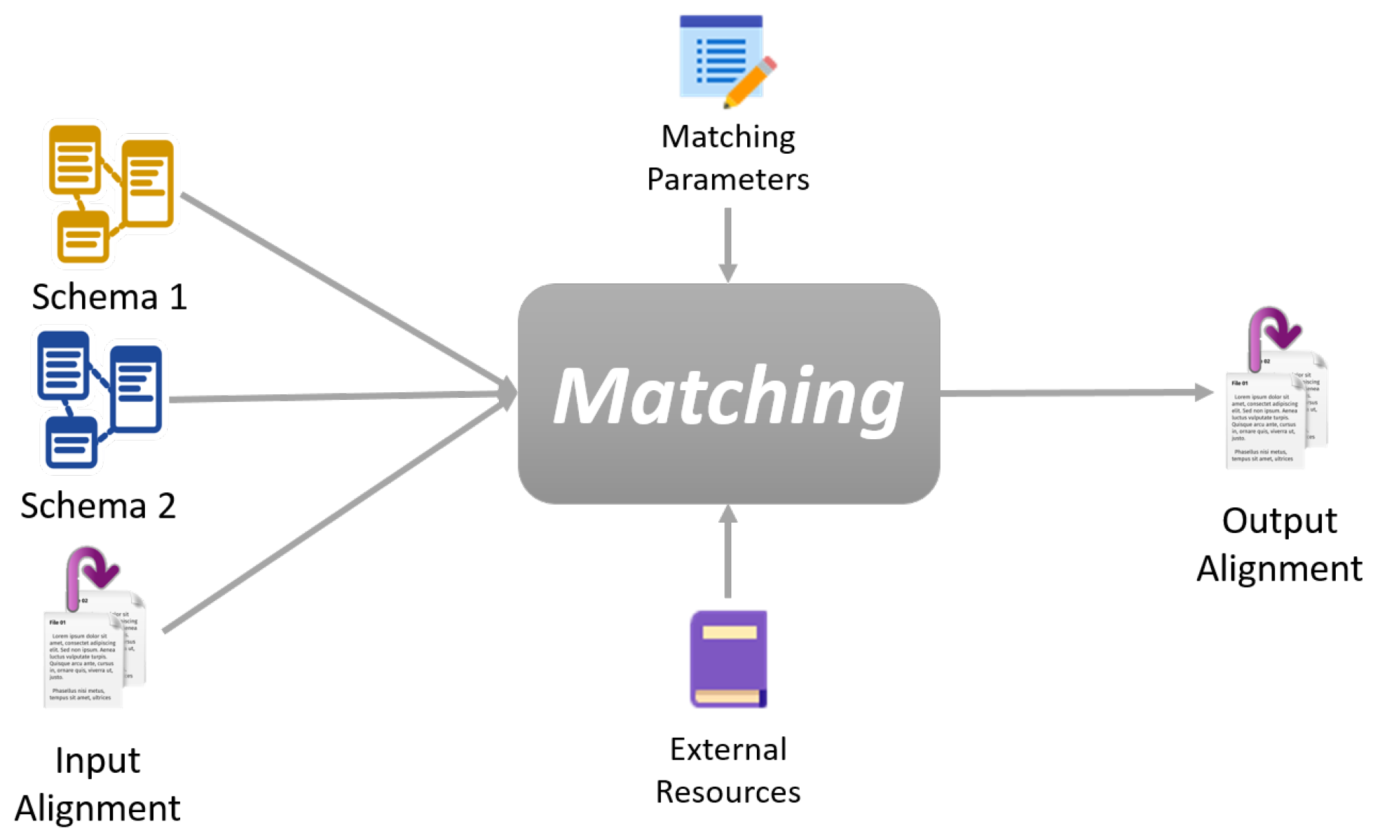
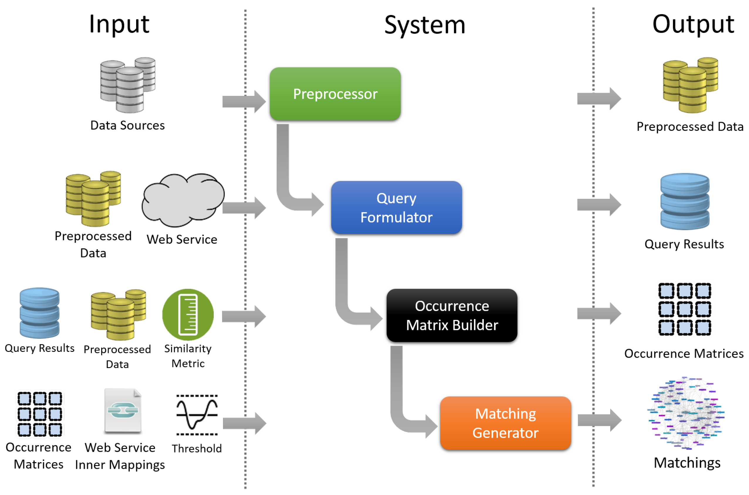
3. An Automatic Matcher for Transportation Datasets

Transportation data instances always refer to real-world objects, e.g., bike stations, bus or train stops, etc. These data are characterized by the description of an object’s geographical location, represented by properties, such as coordinates, addresses, etc. The problem we are faced with is the different representations of this information. We aim at investigating a way to automatically identify and match geospatial information in transportation datasets despite their heterogeneity.

Geocoding services (https://developers.google.com/maps/documentation/geocoding/intr, http://dev.virtualearth.net/REST/v1/Locations/, http://cloudmade.com/documentation/geocoding/, http://www.mapquestapi.com/geocoding/, https://developer.yahoo.com/boss/placefinder/) provide the means of transforming a description of a location (name of a place, coordinates, etc.) to a location on the Earth’s surface via geocoding and reverse geocoding functions. They work as a search engine where the output contains all possible information regarding the location of the queried data.

We believe that exploiting these services can guide the matching process in automatically identifying the geospatial characteristics in the datasets. The idea in general is the following: First we query a geocoding/reverse-geocoding web service with existing instances in order to find matching rules between the queried instances and the web service response. The schema of the web service must be known in advance, so a match between the queried instance and the web service instance will give us some information on the schema of the queried instance. This enables us to detect complex relations between two different representations by using the web service as a mediator. Data sources are mapped to the mediator at first, then by previously-known information about the structure of the mediator, we can detect the required matching rules. Due to the fact that we know how a web service is defined, we can detect n to m relations between the schemas.

Our system consists of four components that include: web service selection and query formulation, co-occurrence matrix construction and, finally, the matching rules generator. A preprocessing step precedes our approach in order to unify the structure representations in each data source and to do some filtering and/or modifications. Here, we use CSV format due to its simplicity. Moreover, since some columns on their own cannot provide meaningful input for a web service query, preprocessing can perform some random combination/split of columns as additional data that may improve the web service query results, e.g., combine street name with city name to get more precise results from the web service. The combination is done automatically and blindly without any prior information about the dataset schema. We note that even when the format is the same, the representation may be totally different. For example, both files are in CSV format, but each represents addresses differently. Figure 3 shows a global view of our system.

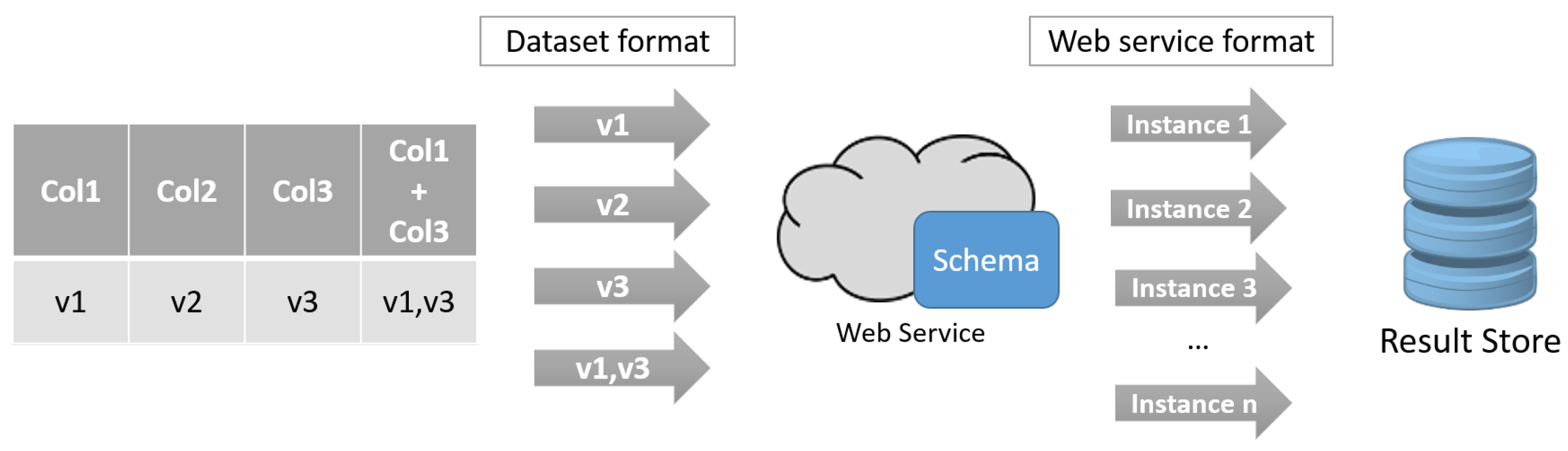
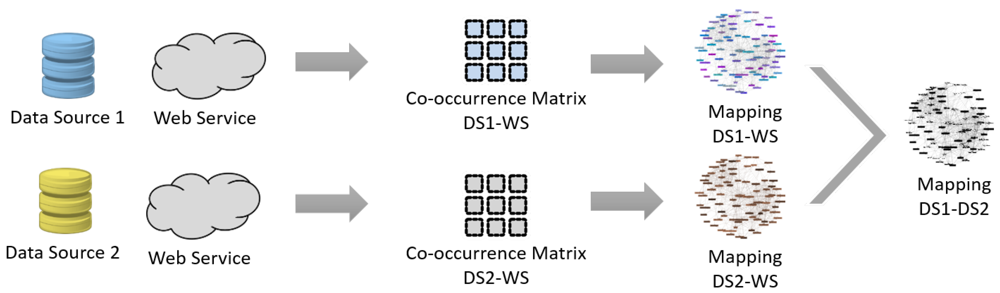
3.1. Web Service-Based Query Formulation

A web service stands as a mediator that maps the data sources. We can identify more formats and representations given a richer web service schema. Therefore, it is required to provide a web service that contains enough representations of addresses to cover any possible encountered format. In addition to the service definition, the knowledge of how the elements are mapped within the web services must be defined. For example, if a web service contains longitude, latitude and a WKT representation of an address, we must specify that a combination of latitude and longitude can be represented in WKT and vice versa. These information are saved as “inner mapping rules” of a web service that are used later in the matching task.

The objective of a query formulator is to query the selected web service with existing instances aiming to get richer information. This step is done on each dataset separately. The query formulator creates a query and sends it to the web service. Separate requests are issued for each column in a row as shown in Figure 4 or by random split/combination of columns previously done in a preprocessing phase, e.g., the fourth column in Figure 4 is the result of preprocessing the file by combining Columns 1 and 3. Note that Col1, Col2, Col3 represent any column names while v1, v2, v3 represent any possible value. The web service results are grouped by the queried columns and stored in a repository for later tasks.

3.2. Co-Occurrence Matrix Construction

Here, we use the web service results and the dataset instances in order to construct a co-occurrence matrix. A co-occurrence matrix is a matrix of n *m rows, where n and m are the number of columns in the dataset and the web service schema, respectively. Each entity in this matrix corresponds to the number of times an element ${\mathrm{a}}_{ij}$ appears at the same time in the column i of the dataset schema and the column j of the web service result schema.

The element comparison is done via a similarity metric [46,47] in which each time a similarity is detected, the corresponding value in the matrix is incremented by one. The higher the value is, the higher the probability that these two columns map to each other. An example of what precedes is shown in Figure 5 with the elements in red representing common occurrences. We see two schemas, one representing a dataset schema and the second representing the web service schema. In the dataset schema, a street is represented by its name and zip-code written in English words, while it is in the web service schema represented by the set {Voie, CodeP and Ville} that stands for {Street, Postal code and City} in French. The co-occurrence matrix lists the columns of both schemas as rows and columns of the array, and each element in the matrix represents the number of times the same value appears in row/column combination. For example, we see that the columns “Voie” and “Street Name” have two values in common, which are “Rue Edme Bouchardon” and “Rue des Chantiers”. To calculate the matrix, we first iterate over each row in the dataset and compare the value of each column with the column values of each row in the web service results. If the similarity between the values exceeds a threshold, the value at the specific row/column index in the matrix is incremented, e.g., if the value at Street Name is similar to the value at Rue, then the cell corresponding to column Street Name and row Rue is incremented.

A co-occurrence matrix is created for each repository, where a repository represents the query results of each column’s instance values. Since we have multiple co-occurrence matrices, we combine them with one aggregated matrix in order to maximize the similarity. This matrix represents the global view on how the columns of each dataset are related to the web service schema based on all of the queries.

3.3. Matching Rules Generation

The calculated co-occurrence matrices capture the possible matching rules between the data sources and the web service and in turn will help with generating the matching rules between their schemas. Here, we iterate over each row and select the highest value. Then, we generate a matching between the corresponding row/column if the number of co-occurrences is higher than some pre-defined threshold.

After having the matching between each dataset and the web service, we use the web service inner mappings to detect how elements from each dataset can be matched together. To illustrate, let us consider two datasets, DS1, DS2, and a web service, WS. Suppose that DS1 contains the columns a1 and b1, the WS schema contains ws1,ws2 and ws3 and DS2 contains a2. Knowing that the column ws3 is the combination of ws1 and ws2, a1 and b1 map to ws1 and ws2, respectively, and a2 maps to ws3, we can conclude that we can map DS1 elements to DS2 elements by the property “a1 combined with b1 is equivalent to a2”. The global picture is shown in Figure 6.

Summing up, the idea is to query each dataset element with a web service that has a known schema and inner mapping rules. We then use the resulting instances to create co-occurrence matrices for each dataset. The matrices are then used to define a matching between each dataset and the web service schema until finally using the inner mapping rules of the web service to create matching rules between the input datasets.

This process is done twice for both datasets. Using the matching rules from D1 to WS and from D2 to WS in addition to the inner mapping rules of WS, the process terminates by showing the matching between D1 and D2.

4. Discovering Semantic Connections between Transportation Datasets

Discovering connections between transportation points of transfer cannot be done using existing interlinking tools. A more complex connection generation process is needed to enable richer and more flexible connection representation. We introduce Link++ (shown in Figure 7), a system that enables flexible connection discovery and customized output definition using connection patterns, custom functions and linking rules. Connection patterns are templates for connection generation used to define both the content and format of a linking process output.

In general, the approach consists of two main phases:

• The definition phase, where users define the connection patterns, the required functions and linking rules.
• The generation phase, where the definitions are taken and applied to the datasets. The rule is applied to the entities, and when valid, a connection will be created and stored in a repository.

In a formal definition, a linking task T requires the following input for the process:

• Input data sources $D1$ and $D2$ representing the datasets to be linked
• O is the custom-defined connection pattern
• R is the linkage rule that defines when a connection must be generated
• F is a set of functions required for the linking task
• L is a set of pre-defined libraries implementing the dependencies of F

The following sections explain in detail the tasks required for an interlinking process.

4.1. Specifying Custom Functions and External Libraries

Users are able to write any functions to be used in their linking rules or similarity calculations. This ensures the flexibility of the approach and the ability to support any interlinking task. In addition, external libraries are supported and can be used within functions’ implementations. These functions may represent a linking rule, a similarity metric, a transformation/preprocessing operations or any other function based on users’ needs. The functions are gathered in a JAVA file accompanied with the used jar libraries.

4.2. Defining a Linking Rule

A linking rule specifies the conditions required to generate a connection between a given pair of entities. The main goal is to apply this rule to each entity pair in order to seek for a match and create the specified connection. Defining a rule requires a set of functions (similarity metrics and preprocessing functions) previously defined by the user. Each rule is defined with a root node that is either an aggregation or a comparison operator and sub-nodes specifying any other function chained in a way to suit the linking task.

An aggregation operator combines the values of different operators/values by applying the specified aggregation method, e.g., max, min, average, etc. It is defined by an aggregation function and a threshold. Each function contains a set of parameters that can be specified from the given data sources or directly by the user. The threshold defines whether the value of the operator must be evaluated as true or false in the linking rule.

Since data sources can be represented in different ways, we can use the transformation operator to modify how values are represented. To this end, we define a function that takes its parameters from the data sources or from the composition of other transformation operators, e.g., lowercase, uppercase, concatenation, round, ceiling, etc.

Finally, the comparison operator is used to define the similarity (or the relatedness) between two properties of the given data sources. A comparison is valid between operators themselves or with other transformation functions, and a threshold defines whether the value is accepted or not for the rule to be valid, e.g., distance, equality, etc.

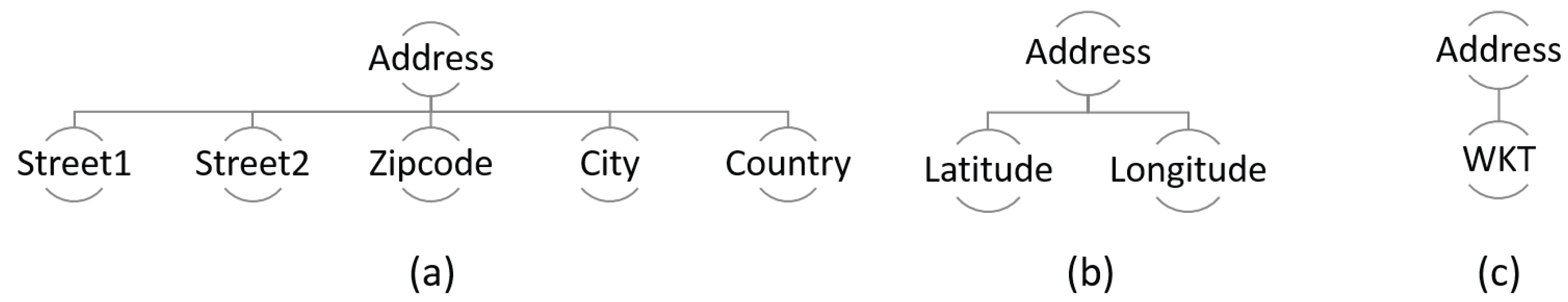
4.3. Configuring a Connection Pattern

The connections are the final outputs of the interlinking task, and it is important to be precise when defining a connection pattern. A pattern specifies the format of the generated connections and the required information they must contain. In other words, it represents a template that will be filled when a connection is instantiated.

A connection pattern is composed of a set of properties, where each property is defined by a function that calculates it. Function parameters can be the inputs from the data sources or predefined by the rule composer. A connection pattern is freely chosen by a user according to the interlinking task and the post-processing needs. The formal definition of a connection pattern O is as follows:

Definition 1.

Let D₁ and D₂ be two data sources. Given V any data type and F a set of custom functions required to generate the patterns, Pr is a set of properties where each property is represented by a property name n, a value v and a corresponding function f, which calculates the property value during the generation process.

$$Pr=\left\{\right(n,v,f\left)\right|n\in String,v\in Vf\in F\}$$

(1)

A connection pattern is formalized as:

$$O=(d_1,d_2,pr)|d_1\in D_1,d_2\in D_2,pr\subseteq Pr$$

(2)

We will give a demonstration case with a real scenario of defining both the linking rule and the connection pattern in Section 5.

Once the configuration step is completed, the connection discovery is performed as described in the sequel.

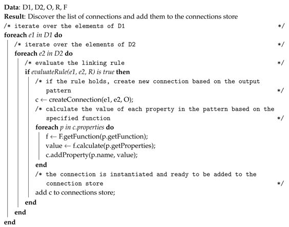
4.4. Connection Discovery Algorithm

Algorithm 1 represents the pseudo-code of the implemented linking process.

The algorithm iterates over each pair of entities in the two data sources and evaluates the linking rule between them. Based on the rule evaluation, the algorithm decides if a connection must be created or not. If a rule is triggered, a new connection is generated by evaluating the connection pattern and applying the corresponding function of each property. The values are calculated by the specified functions in the output pattern, and their parameters are filled from the currently-compared entities. Here, we instantiate the connection and fill in its information from the return values of the functions. The connection is stored in a specified repository, and the algorithm continues on the remaining pairs until all are treated.

Algorithm 1: Connection discovery algorithm.

In the worst cases, the time complexity of the algorithm is O(n * m), where n and m are the sizes of the input datasets. The storage complexity (in terms of data pages) is the same as a nested loop join in databases that is equal to the size of the smallest dataset + one page, which usually fits in memory. This complexity may be reduced by using some pre-filtering techniques that the system may offer in a future version; for instance, using a spatial index to replace the inner loop by a search in an index (which reduces the cost to log(n)). Then, the specific rules and function defined by the user will be applied in a refinement phase automatically by the system.

Both the connection pattern and the linking rule files are described in XML files that conform a data type definition (DTD) ; custom functions are written using JAVA (users can write any JAVA file and use the defined methods in his/her connection pattern or rule), and the output is generated in RDF. An example with real linked datasets is presented in the evaluation section; it illustrates the configuration process and shows an instance of the XML files (output pattern and rule).

We have implemented our approach, and an executable version of the system can be found online via the link https://github.com/alimasri/link-plus-plus.git; in addition to a video tutorial on: https://youtu.be/u2gr7Wa4eT4.

5. Evaluation

We evaluate both of our two approaches using two datasets representing transportation companies in the Paris area, SNCF and Autolib, a railway company and a car sharing service, respectively.

The main idea is to provide missing connections between stops belonging to different transportation modes and see how this would improve users’ trip planning. We first show how we automatically discover the geospatial properties between the two datasets and then how we can use this information to link them using the proposed interlinking approach.

The input data are collected from the open data portals for SNCF (http://gtfs.s3.amazonaws.com/transilien-archiver_20160202_0115.zip) and Autolib (http://opendata.paris.fr/explore/dataset/stations_et_espaces_autolib_de_la_metropole_parisienne/) in CSV representations. The number of instances in each of the SNCF and Autolib datasets is 1067 and 869, respectively. Figure 8 shows the original schema of the datasets.

5.1. Automatic Schema Matching

We will describe the process of automatically detecting the geospatial properties of both datasets according to the steps shown in Section 3.

In a preprocessing phase, we split columns containing special characters (commas, semi-colons) into two or more columns named by the original column’s name with an incremented value concatenated to its end. Therefore here Autolib’s column “Cordonnees geo” is split into two columns “Cordonnees geo 0” and “Cordonnees geo 1”.

For the web service selection, we chose Google’s geocoding web service (https://developers.google.com/maps/documentation/geocoding) with one function on top implemented by us to filter out the results in a simple schema that consists of three columns: formatted-address (representing a textual address representation), lng (longitude) and lat (latitude).

The query formulator queries the web service with each column’s value for all of the existing rows, then groups the results by column names and saves them into a repository. The total number of issued queries is 20,185 divided into 8536 and 11,649 for SNCF and Autolib, respectively.

One co-occurrence matrix is constructed for each column ignoring columns that gave no results from the web service. The used similarity metric is the Levenshtein distance in order to show how a simple similarity metric can give us good results. However, more complex metrics can be used to increase the precision of the similarity calculation. An aggregation matrix is then created by calculating the mean value of all co-occurrence matrices’ values. The resulting matrices for SNCF and Autolib are shown in

Table 2. SNCF’s co-occurrence matrix.

	Formatted_Address	Lat	Lng
stop_id	0	35.750	39.625
stop_code	0	0	0
stop_name	11.875	0	0
stop_desc	1.375	0	0
stop_lat	0	296.875	5.375
stop_lon	0	0.625	14.375
location_type	0	0	0
parent_station	0	0	0

and

Table 3. Autolib’s co-occurrence matrix.

	Formatted_Address	Lat	Lng
ID	0	12.364	0.364
Identifiant Autolib’	18.818	0	0
Rue	2.545	0	0
Code postal	0	0	0
Ville	27.636	0	0
Coordonnees geo_0	0	5876.818	523.909
Coordonnees geo_1	0	545.636	916.636
Emplacement	0	0	0
Autolib’	1397	0	0
Tiers	0	0	0
Abri	0	0	0

.

In order to generate the matching rules, we iterate over each row, get the maximum value and assign a matching between the corresponding row/column pair. Using Table 2 and Table 3, we obtain the following matching rules between each of them and the web service; for SNCF: (stop-id, lng), (stop-name, formatted-address), (stop-desc, formatted-address), (stop-lat, lat) and (stop-lon, lng); for Autolib: (ID, lat), (Identifiant Autolib’, formatted-address), (Rue, formatted-address), (Ville, formatted-address), (Cordonnees geo-0, lat), (Cordonnees geo-1, lng) and (Autolib’, formatted-address). The execution time took around 3.5 min on the given datasets, including a one-second cool-down per each ten queries to comply with the restrictions of the web service.

Analyzing the results for SNCF, our system correctly obtained matching of the latitude and longitude properties. Moreover, since the stop-name and stop-dec are normally names of the corresponding area, they were detected as geospatial properties, as well. Regarding the stop id, this false positive matching rule can be solved by combining the results with some constraint-based approaches. Regarding Autolib, the matching rules detected correct relations between rue and formatted-address and the same for the latitude and longitude with cordonnees geo 0 and 1. The false positive matches were: (ville, formatted-address), (ID, lat), (Identifiant Autolib’, formatted-address) and, finally, (Autolib’, formatted-address). The false negatives’ matching rules can also be discarded using constraint-based approaches, for example by removing matching from repeated column values or id columns, etc.

The results show a 100% precision and 80% recall for SNCF and 100% precision 42% and recall for Autolib. Matching results could be improved in different ways: (i) choosing richer web services; (ii) refining the preprocessing of the output; or (iii) using alternative similarity metrics. Combining both matching rules, we can deduce the following valid rules between SNCF and Autolib: “Cordonnees geo” from Autolib maps to the combination of (stop-lat,stop-lon) in SCNF; “Rue” from Autolib maps to “stop-desc” in SNCF.

We tested the algorithm on other datasets to validate it. The chosen datasets are hospital locations in the U.K. and points of interests (POI)in Paris, in addition to the previous train and car stations. The idea here is that this approach can help in checking if the datasets contain geospatial information in addition to the ability to identify them and the relation to other datasets. This can be used in uses cases such as finding the nearest hospital from an accident location or finding some POIs near a hotel, etc. The results are shown in

Table 4. Evaluation of the matching algorithm.

	Precision	Recall	F-Measure
SNCF 1	1	0.8	0.88
Autolib 2	1	0.42	0.59
Hospitals 3	1	0.8	0.88
POI 4	1	1	1

¹ http://gtfs.s3.amazonaws.com/transilien-archiver_20160202_0115.zip; ² http://opendata.paris.fr/explore/dataset/stations_et_espaces_autolib_de_la_metropole_parisienne/; ³ https://data.gov.uk/dataset/hospitals; ⁴ http://opendata.paris.fr/explore/dataset/zones-touristiques-internationales/export/.

.

5.2. Link Discovery

After the detection of the geospatial properties, the following process is to find the transportation connections between both datasets. In transportation networks, a connection can be described as an accessible path from one transportation point of transfer to another. A point of transfer is any stop that allows users to change a transportation unit or mode. A connection contains properties describing both the departure and arrival stops in addition to other properties. We define a transportation connection as one of the following two types:

• Timetable connection that has specific departure and arrival times. This type of connection will be referred to as a scheduled connection. It has the following properties: departure-time, arrival-time, departure-stop and arrival-stop.
• Other connections that have no schedule information and for which availability is not restricted by timing constraints. We will refer to these connections as unscheduled connections. They have the following properties: departure-stop, arrival-stop and distance.

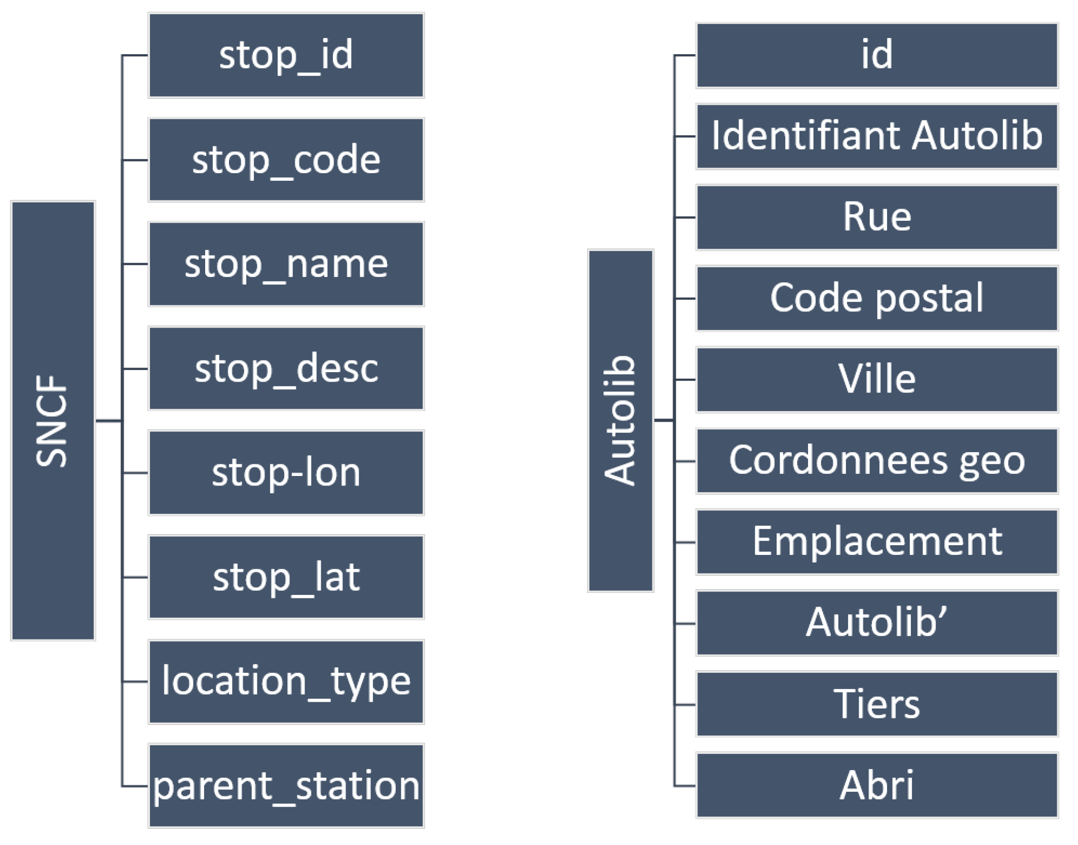
5.2.1. Data Preparation

In this phase, the goal is to represent the timetable information in a format compatible with our definition of connection. Instead of designing a network by a series of stops or other representations, we want to represent it by a series of connections between stops. Since SNCF is a public transportation company with data described in timetables, the task here is to extract scheduled connections from the given data. To this end, we have proposed an algorithm that transforms timetable data from GTFS files into scheduled connections. The algorithm iterates over the timetable information for each stop and creates a connection that starts from a departure stop at a departure time and ends with an arrival stop with the specified time. The process is repeated to a predefined date range to limit the number of connections created.

In case of Autolib, we do not have timetable information, so we need a way to discover the connections between its stops. Using our approach, we can match Autolib’s dataset with itself (in order to know when a Autolib station is reachable from an another) to discover these unscheduled connections between. Since the configuration task is common and independent, the following section describes how to use our approach to discover the unscheduled connections for Autolib-Autolib and Autolib-SNCF.

5.2.2. Discovering New Connections

Two tasks are required one for Autolib-Autolib connections and one for Autolib-SNCF connections. In this example, unscheduled connections are driving or walking connections between Autolib-VELIBand Autolib-SNCF, respectively. We use our approach to search for connections that match a predefined criteria. Since our approach works on RDF data, we have used the DataLift [34] platform to transform both SNCF stops and VELIB CSV files into RDF turtle formats. In the sequel, we describe in detail all of the required tasks to achieve our goal.

• Defining custom functions: Our system is flexible as it allows users to create any custom function to be used in the linking task. Users can use external dependencies, as well. In our example, we define the functions getWalkingDistance, getWalkingTime, getDrivingDistance and getDrivingTime. In a real scenario, we get this information from a web service, such as Google’s distance matrix API (https://developers.google.com/maps/documentation/distance-matrix/), However, due to the query limit, we have chosen to implement them by local functions based on mathematical calculations (http://www.movable-type.co.uk/scripts/latlong.html).
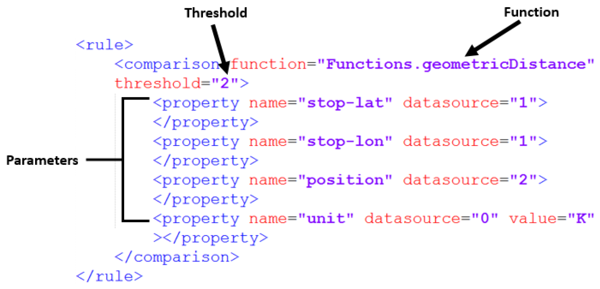
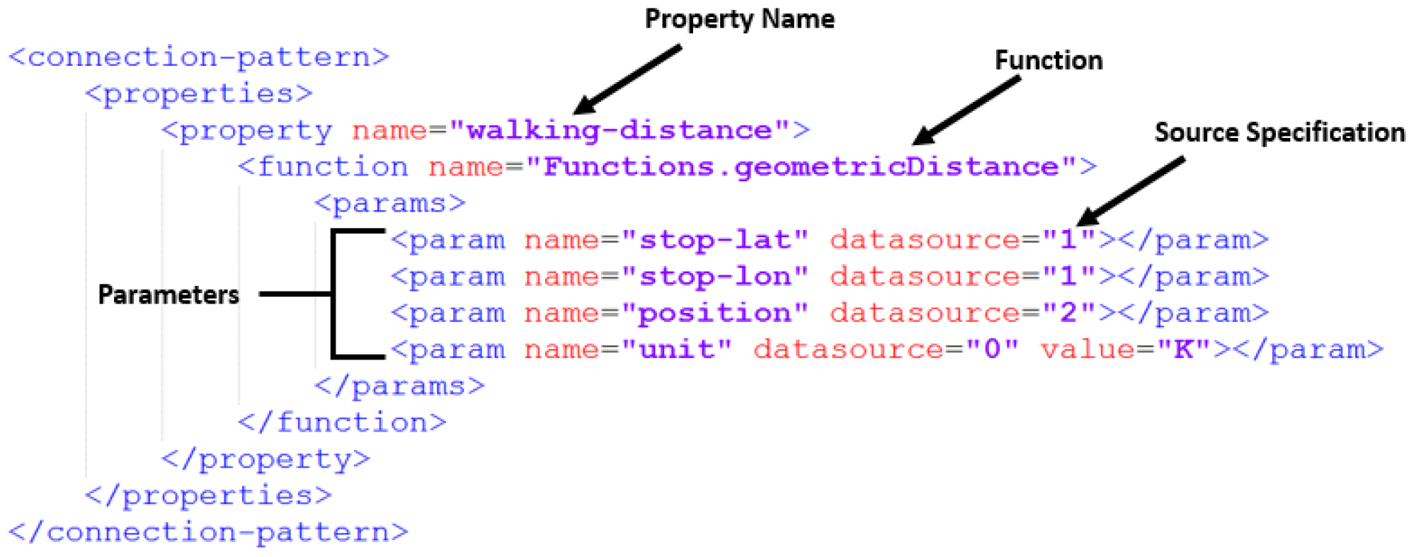
• Define the linking rules: Recall that the linking rule describes the condition that triggers the creation of a connection. Two rules are required, one for Autolib-Autolib and the other for Autolib-SNCF. For the first one, the condition of the defined rule is the following: “If a driving path exists within 200 km (the time before the battery is totally discharged), create a connection”. For Autolib-SNCF connections, the rule is: “If a walking path exists from one stop to another within one kilometer, create a connection”. Rules are written in XML format, and the functions that calculate the walking distance and time are referenced from the custom functions file. We note that the parameters “200 km” and “1 km” are given by the user who is responsible for the configuration. We set these parameters as the maximum feasible scope for a person to ride the car or walk from one station to another. Figure 9 shows an example of how a rule can be defined.
• Defining the connection pattern: We define the output generated by the system at each valid rule. We have chosen the following properties to be represented in a connection pattern: source-id, target-id, walking/driving distance and walking/driving time. This pattern is the same for both tasks, and an example is shown in Figure 10.

Executing these tasks with the above configuration enabled us to enrich the network with discovering 535,966 internal connections between Autolib car stations and 272 new connections between the two different transportation modes SNCF and Autolib. We will illustrate hereafter how to use these connections to calculate the earliest arrival time (EAT).

5.2.3. Calculating Routes Using Discovered Connections

EAT is the earliest time we can reach all stops in a transportation network given a departure stop and time. We have chosen this approach to get a broad view on how the newly-introduced connections can massively affect a large network. We have used the connection scan algorithm (CSA) [48] as an EAT implementation, since it matches with our notion of connection. In short, CSA works by receiving a stream of connections ordered by departure time and chooses the fastest way to reach one stop from another. Due to the fact that the connections are pre-sorted and can be accessed one by one in a single iteration, CSA is faster and more scalable than other existing algorithms. However, it has some limitations in our case. Firstly, it only supports timetable networks, which makes it unable to compute trips, including other services. Secondly, it does not support unscheduled connections. It only supports one footpath transition between two points of transfers. It is therefore not possible to combine scheduled connections, unscheduled connections and footpaths to create a more optimized trip.

CSA handles only public transportation networks with footpaths. In order to support multimodality, we have introduced unscheduled connections beside the ones based on timetables. We have also enabled multiple unscheduled connections between multiple points of transfer. The unscheduled connections are created when a connection is reached. For each iteration, all of the available unscheduled connections from an arrival stop are checked to create scheduled connections by setting the departure time to be equal to the arrival time at the station; to this is added the minimum transfer duration and the arrival time for the unscheduled connection.

We fed our new algorithm with both scheduled and unscheduled connections and tested the estimated arrival time for each stop. To check the effects of introducing generated connections, we have calculated the estimated arrival times with and without them, and we have compared the results. Figure 11 represents the estimated arrival time for every stop starting from the SNCF departure stop DUA8711617. The intuition is that the lower the value, the earlier a passenger can reach a stop point starting from a departure station.

Analyzing Figure 11 shows that using the generated connections and integrating them in the transportation network can reduce the estimated arrival time. Therefore, introducing these connections decreases the waiting time for passengers and results in more optimized trips. We can now consider new types of mobility that were not previously taken into account (bike sharing, car sharing, etc.). This can be used to fit to passengers profiles by combining the appropriate connections while planning trips. Passengers will be able to define connection types, modes and find the best trip type.

Compared to the existing link discovery frameworks, our approach succeeded in discovering links with richer representations and extendable properties that can be used for numerous tasks (EAT in our example).

6. Conclusions

The diversity of transportation systems and services raises the need for a broader integrated view of the transportation network. This in turn can provide multimodality that greatly improves passenger’s experience with more optimized and customizable trips.

In this paper, we proposed an approach to automatically detect geospatial data between transportation data sources in addition to a way to provide rich semantic connections between their entities. This enables a better way for transportation systems to access information about new services and integrate them with their own network.

We evaluated our approach with a scenario of integrating a car sharing and a train station company in France. The result shows that the approach was able to detect the geospatial entities and find relations between the dataset schemas. Moreover, using the rich generated links between the datasets, the integration of the new mode of transportation improved the earliest arrival time at each stop.

In the future, we want to adapt the approach to handle the dynamicity of the connections. This will make us able to maintain the status of existing connections and handle new services, such as dynamic ride-sharing, car sharing, etc. The problem here is how to track connections’ evolution in real time. How can we make use of external events that may affect their use, etc.? Furthermore, some speed optimization is to be considered for both the automatic matching and interlinking approaches. We will target data sampling to reduce the web service calls and a smarter query formulator to more efficiently get relevant results from the web service. Integrating geospatial querying solutions shown in [25] may help with increasing the accuracy of the query formulator. The use of a web service to bridge the gap between different dataset representations could apply to other domains as long as web services are provided for these datasets.

References

1. Gurstein, M.B. Open data: Empowering the empowered or effective data use for everyone? First Monday 2011. [Google Scholar] [CrossRef]
2. Bizer, C.; Heath, T.; Berners-Lee, T. Linked data-the story so far. Int. J. Semant. Web Inf. Syst. 2009, 5, 1–22. [Google Scholar] [CrossRef]
3. Plu, J.; Scharffe, F. Publishing and linking transport data on the web: Extended version. In Proceedings of the First International Workshop on Open Data, Nantes, France, 25 May 2012; pp. 62–69.
4. Consoli, S.; Mongiovì, M.; Recupero, D.R.; Peroni, S.; Gangemi, A.; Nuzzolese, A.G.; Presutti, V. Producing linked data for smart cities: The case of Catania. Big Data Res. 2016. [Google Scholar] [CrossRef]
5. Euzenat, J. An API for ontology alignment. In The Semantic Web–ISWC 2004; Springer: Berlin/Heidelberg, Germany, 2004; pp. 698–712. [Google Scholar]
6. Euzenat, J.; Shvaiko, P. Ontology Matching; Springer: Berlin/Heidelberg, Germany, 2007. [Google Scholar]
7. Shvaiko, P.; Euzenat, J. A survey of schema-based matching approaches. In Journal on Data Semantics IV; Springer: Berlin/Heidelberg, Germany, 2005; pp. 146–171. [Google Scholar]
8. Segev, A.; Kantola, J.; Jung, C.; Lee, J. Analyzing multilingual knowledge innovation in patents. Expert Syst. Appl. 2013, 40, 7010–7023. [Google Scholar] [CrossRef]
9. Rahm, E.; Bernstein, P.A. A survey of approaches to automatic schema matching. VLDB J. 2001, 10, 334–350. [Google Scholar] [CrossRef]
10. Kalfoglou, Y.; Schorlemmer, M. Ontology mapping: The state of the art. Knowl. Eng. Rev. 2003, 18, 1–31. [Google Scholar] [CrossRef]
11. Wache, H.; Voegele, T.; Visser, U.; Stuckenschmidt, H.; Schuster, G.; Neumann, H.; Hübner, S. Ontology-based integration of information-a survey of existing approaches. In IJCAI-01 Workshop: Ontologies and Information Sharing; Citeseer: Princeton, NJ, USA, 2001; pp. 108–117. [Google Scholar]
12. Bernstein, P.A.; Madhavan, J.; Rahm, E. Generic schema matching, ten years later. Proc. VLDB Endow. 2011, 4, 695–701. [Google Scholar]
13. Shvaiko, P.; Euzenat, J. Ontology matching: State of the art and future challenges. IEEE Trans. Knowl. Data Eng. 2013, 25, 158–176. [Google Scholar] [CrossRef] [Green Version]
14. Daskalaki, E.; Flouris, G.; Fundulaki, I.; Saveta, T. Instance matching benchmarks in the era of Linked Data. Web Semant. Sci. Serv. Agents World Wide Web 2016, 39, 1–14. [Google Scholar] [CrossRef]
15. Zaiss, K.; Conrad, S.; Vater, S. A benchmark for testing instance-based ontology matching methods. In Proceedings of the 17th International Conference Knowledge Engineering and Knowledge Management, Lisbon, Portugal, 11–15 October 2010.
16. Dai, B.T.; Koudas, N.; Srivastava, D.; Tung, A.K.; Venkatasubramanian, S. Validating multi-column schema matchings by type. In Proceedings of the 2008 IEEE 24th International Conference on Data Engineering, Cancun, Mexico, 7–12 April 2008.
17. Warren, R.H.; Tompa, F.W. Multi-column substring matching for database schema translation. In Proceedings of the 32nd International Conference on Very Large Data Bases, Seoul, Korea, 12–15 September 2006.
18. Bohannon, P.; Elnahrawy, E.; Fan, W.; Flaster, M. Putting context into schema matching. In Proceedings of the 32nd International Conference on Very Large Data Bases, Seoul, Korea, 12–15 September 2006.
19. Partyka, J.; Parveen, P.; Khan, L.; Thuraisingham, B.; Shekhar, S. Enhanced geographically typed semantic schema matching. Web Semant. Sci. Serv. Agents World Wide Web 2011, 9, 52–70. [Google Scholar] [CrossRef]
20. Li, W.S.; Clifton, C. SEMINT: A tool for identifying attribute correspondences in heterogeneous databases using neural networks. Data Knowl. Eng. 2000, 33, 49–84. [Google Scholar] [CrossRef]
21. Embley, D.W.; Xu, L.; Ding, Y. Automatic direct and indirect schema mapping: Experiences and lessons learned. ACM SIGMOD Rec. 2004, 33, 14–19. [Google Scholar] [CrossRef]
22. Brauner, D.F.; Intrator, C.; Freitas, J.C.; Casanova, M.A. An instance-based approach for matching export schemas of geographical database web services. In Proceedings of the IX Brazilian Symposium on Geoinformatics, São Paulo, Brazil, 25–28 November 2007.
23. Feliachia, A.; Abadieb, N.; Hamdic, F. Matching and Visualizing Thematic Linked Data: An Approach Based on Geographic Reference Data; IOS Press: Amsterdam, The Netherlands, 2014. [Google Scholar]
24. Al-Salman, R.; Dylla, F.; Fogliaroni, P. Matching geo-spatial information by qualitative spatial relations. In Proceedings of the 1st ACM SIGSPATIAL International Workshop on Crowdsourced and Volunteered Geographic Information, Redondo Beach, CA, USA, 7–9 November 2012.
25. Smid, M.; Kremen, P. OnGIS: Semantic Query Broker for Heterogeneous Geospatial Data Sources. Open J. Semant. Web (OJSW) 2016, 3, 32–50. [Google Scholar]
26. Lüscher, P.; Burghardt, D.; Weibel, R. Matching road data of scales with an order of magnitude difference. In Proceedings of the XXIII International Cartographic Conference, Moscow, Russia, 4–10 August 2007.
27. Yi, S.; Huang, B.; Wang, C. Pattern matching for heterogeneous geodata sources using attributed relational graph and probabilistic relaxation. Photogramm. Eng. Remote Sens. 2007, 73, 663–670. [Google Scholar] [CrossRef]
28. Li, J.; Wang, Z.; Zhang, X.; Tang, J. Large scale instance matching via multiple indexes and candidate selection. Knowl.-Based Syst. 2013, 50, 112–120. [Google Scholar] [CrossRef]
29. Jain, P.; Hitzler, P.; Sheth, A.P.; Verma, K.; Yeh, P.Z. Ontology alignment for linked open data. In The Semantic Web–ISWC 2010; Springer: Berlin/Heidelberg, Germany, 2010; pp. 402–417. [Google Scholar]
30. Ferrara, A.; Nikolov, A.; Noessner, J.; Scharffe, F. Evaluation of instance matching tools: The experience of OAEI. Web Semant. Sci. Serv. Agents World Wide Web 2013, 21, 49–60. [Google Scholar] [CrossRef]
31. Isele, R.; Bizer, C. Active learning of expressive linkage rules using genetic programming. Web Semant. Sci. Serv. Agents World Wide Web 2013, 23, 2–15. [Google Scholar] [CrossRef]
32. Scharffe, F.; Euzenat, J. MeLinDa: An interlinking framework for the web of data. Artif. Intell. 2011. [Google Scholar]
33. Le Grange, J.J.; Lehmann, J.; Athanasiou, S.; Garcia-Rojas, A.; Giannopoulos, G.; Hladky, D.; Isele, R.; Ngomo, A.C.N.; Sherif, M.A.; Stadler, C.; et al. The GeoKnow Generator: Managing Geospatial Data in the Linked Data Web. In Proceedings of the Linking Geospatial Data, London, UK, 5–6 March 2014.
34. Scharffe, F.; Atemezing, G.; Troncy, R.; Gandon, F.; Villata, S.; Bucher, B.; Hamdi, F.; Bihanic, L.; Képéklian, G.; Cotton, F.; et al. Enabling linked data publication with the Datalift platform. In Proceedings of the AAAI Workshop on Semantic Cities, Toronto, ON, Canada, 22–23 July 2012.
35. Hamdi, F.; Abadie, N.; Bucher, B.; Feliachi, A. Geomrdf: A geodata converter with a fine-grained structured representation of geometry in the web. Int. Workshop Geospat. Linked Data arXiv 2015. [Google Scholar]
36. Volz, J.; Bizer, C.; Gaedke, M.; Kobilarov, G. Silk-A Link Discovery Framework for the Web of Data. Linked Data Web 2009. [Google Scholar] [CrossRef]
37. Ngomo, A.C.N.; Auer, S. Limes-a time-efficient approach for large-scale link discovery on the web of data. In Proceedings of the 22nd International Joint Conference on Artificial Intelligence, Barcelona, Spain, 16–22 July 2011.
38. Raimond, Y.; Sutton, C.; Sandler, M.B. Automatic interlinking of music datasets on the Semantic Web. In Proceedings of the Linked Data on the Web (LDOW 2008), Beijing, China, 22 April 2008.
39. Hassanzadeh, O.; Lim, L.; Kementsietsidis, A.; Wang, M. A declarative framework for semantic link discovery over relational data. In Proceedings of the 18th International Conference on World Wide Web, Madrid, Spain, 20–24 April 2009.
40. Jaffri, A.; Glaser, H.; Millard, I. Managing URI synonymity to enable consistent reference on the Semantic Web. In Proceedings of the IRSW2008—Identity and Reference on the Semantic Web, Tenerife, Spain, 2 June 2008.
41. Scharffe, F.; Liu, Y.; Zhou, C. Rdf-ai: An architecture for rdf datasets matching, fusion and interlink. In Proceedings of the IJCAI 2009 Workshop on Identity, Reference, and Knowledge Representation (IR-KR), Pasadena, CA, USA, 11 July 2009.
42. Arnold, P.; Rahm, E. Enriching ontology mappings with semantic relations. Data Knowl. Eng. 2014, 93, 1–18. [Google Scholar] [CrossRef]
43. Athanasiou, S.; Hladky, D.; Giannopoulos, G.; Garcia Rojas, A.; Lehmann, J. GeoKnow: Making the web an exploratory place for geospatial knowledge. ERCIM News 2014, 96, 12–13. [Google Scholar]
44. Stadler, C.; Lehmann, J.; Höffner, K.; Auer, S. Linkedgeodata: A core for a web of spatial open data. Semant. Web 2012, 3, 333–354. [Google Scholar]
45. Batet, M.; Harispe, S.; Ranwez, S.; Sánchez, D.; Ranwez, V. An information theoretic approach to improve semantic similarity assessments across multiple ontologies. Inf. Sci. 2014, 283, 197–210. [Google Scholar] [CrossRef]
46. Cheatham, M.; Hitzler, P. String similarity metrics for ontology alignment. In Proceedings of the 12th International Semantic Web Conference, Sydney, Australia, 21–25 October 2013.
47. Lesot, M.J.; Rifqi, M.; Benhadda, H. Similarity measures for binary and numerical data: A survey. Int. J. Knowl. Eng. Soft Data Paradig. 2008, 1, 63–84. [Google Scholar] [CrossRef]
48. Dibbelt, J.; Pajor, T.; Strasser, B.; Wagner, D. Intriguingly simple and fast transit routing. In Experimental Algorithms; Springer: Berlin/Heidelberg, Germany, 2013; pp. 43–54. [Google Scholar]
Figure 1. Different address representations.
Ijgi 06 00029 g001
Figure 2. The matching operation.
Ijgi 06 00029 g002
Figure 3. A system for the automatic detection of geospatial information.
Ijgi 06 00029 g003
Figure 4. Querying web services to obtain instances with richer data.
Ijgi 06 00029 g004
Figure 5. Example of co-occurrence matrix calculation.
Ijgi 06 00029 g005
Figure 6. Discovering matching rules between datasets using a web service as a mediator. DS, dataset; WS, web service.
Ijgi 06 00029 g006
Figure 7. Link++: An approach for flexible and customizable connection generation.
Ijgi 06 00029 g007
Figure 8. The original schemas of SNCF and Autolib datasets.
Ijgi 06 00029 g008
Figure 9. An example of rule definition in XML.
Ijgi 06 00029 g009
Figure 10. An example of a connection pattern in XML.
Ijgi 06 00029 g010
Figure 11. The estimated arrival time for each stop with and without our created connections.
Ijgi 06 00029 g011