Detection of Electronic Anklet Wearers’ Groupings throughout Telematics Monitoring

Abstract

Ankle bracelets (anklets) imposed by law to track convicted individuals are being used in many countries as an alternative to overloaded prisons. There are many different systems for monitoring individuals wearing such devices, and these electronic anklet monitoring systems commonly detect violations of circulation areas permitted to holders. In spite of being able to monitor individual localization, such systems do not identify grouping activities of the monitored individuals, although this kind of event could represent a real risk of further offenses planned by those individuals. In order to address such a problem and to help monitoring systems to be able to have a proactive approach, this paper proposes sensor data fusion algorithms that are able to identify such groups based on data provided by anklet positioning devices. The results from the proposed algorithms can be applied to support risk assessment in the context of monitoring systems. The processing is performed using geographic points collected by a monitoring center, and as result, it produces a history of groups with their members, timestamps, locations and frequency of meetings. The proposed algorithms are validated in various serial and parallel computing scenarios, and the correspondent results are presented and discussed. The information produced by the proposed algorithms yields to a better characterization of the monitored individuals and can be adapted to support decision-making systems used by authorities that are responsible for planning decisions regarding actions affecting public security.

1. Introduction

The use of electronic anklets by investigated and convicted persons has been applied by the Brazilian enforcement authorities to try to reduce mass incarceration in the country. 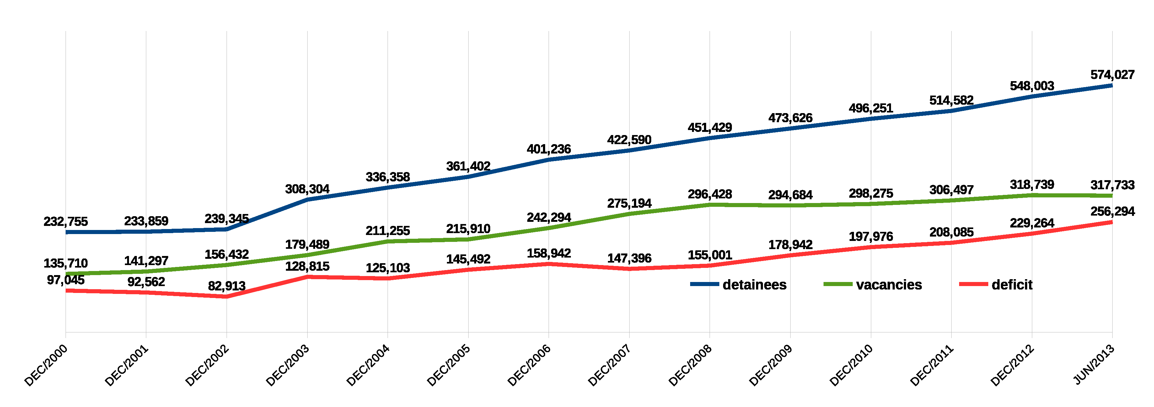According to December 2013 data from the National Penitentiary Department (DEPEN - Departamento Penitenciário Nacional ) of the Ministry of Justice, Brazil has one of the largest prison populations in the world, with 581,507 inmates [1]. The number of people incarcerated increased 52% in the 2005–2013 period. At the same time, there is a growing deficit of prison capacity (Figure 1), resulting in overloaded prisons. In Figure 1, the presented information was extracted from the Penitentiary Information Integrated System (INFOPEN - Sistema Integrado de Informação Penitenciária) from DEPEN, last updated in July 2014.

Sentence serving effectiveness inside current overloaded prisons has been stressed by indoctrinators, who claim that such prisons, together with their management methods, are a failure as a means of rehabilitating offenders. Moreover, these indoctrinators argue that this institution has not been proven for behavior rehabilitation, but serves on the contrary as a “true school for criminals”.

In principle, prison sentence serving in Brazil must follow well-defined parameters regarding the respect to and the dignity of the prisoner, a requirement of the entire prison community, thus respecting the limitations arising from the sentence, as well as social, economic and cultural rights. Therefore, the possibility that the convict regains her or his dignity through social interaction is one of the goals that guides all sentence serving schemes and, consequently, law enforcement. It seems that a remedy contributing to rehabilitation is to re-socialize a convict, asking the State to rigorously perform the monitoring of this process.

In this sense, the use of convict surveillance by telematics means has proven to be a viable alternative for monitoring sentence servings, thus leading to the development of innovations in the control of individuals who violate criminal laws. One such alternative is the monitoring of convicts who are required to wear electronic anklets that integrate GPS sensors, a form of surveillance that proved effective both in the United States and Europe [2]. Thus, criminal justice systems use GPS devices to monitor offenders, individuals that are out of prison, but forced by law to wear anklets that report their locations to monitoring agencies [3]. This electronic monitoring of convicts may be considered an effective means of social reintegration, which can be gradual since the individual monitoring can be adapted to different sentence serving regimes, as for instance the closed, semi-open and open regimes in the Brazilian legal system.

The use of electronic monitoring brings a breakthrough to the criminal enforcement system. First, from the social point of view, it provides better reintegration for the rehabilitating convict into a society that otherwise is not prepared for dialog and much less prone to assist convicted individuals in the social reintegration process. Furthermore, electronic monitoring answers the issue of the intimate life privacy of the monitored persons and their families. Taking into account that currently “35% of the prison population in Brazil is made up of pre-trial detainees and 30% of inmates were sentenced for committing crimes without violence or serious threat” [4], electronic monitoring is presented as a key to evolving the penitentiary system.

Another advantage is that electronic monitoring saves public money expenses regarding the prison system, especially considering the issue of the operational effort and cost of surveillance. A succeeding convict monitoring system can reduce, to a great extent, the number of gradual steps to freedom that are currently employed in prison regime progression, including temporary leaves. Similar savings can be obtained from other applications for convict monitoring without direct supervision.

The architectures used in monitoring systems with electronic anklets follow, in general, the following workflow: geodesic coordinates collected by the anklet devices are sent through a GSM/General Packet Radio Service (GPRS) data transmission network via mobile network operators, thus pushing the data to the monitoring center. This latter processes geographic data from the anklets and issues reports and alerts for the relevant authorities to take action in accordance with the policies of each state. The most common monitoring information output is the indication of a tracked offender entering forbidden geographical areas.

Following, we briefly describe the main elements that are part of the structure used for an anklet monitoring system, since these elements are necessary for understanding the system operation and its respective data stream:

• GPS:
  Global Navigation Satellite Systems (GNSS) comprise constellations of satellites that by transmitting signals to a receiver, make it possible to determine its coordinates. These signals, which are transmitted at specific frequencies, possess peculiar characteristics that allow their identification by receivers, characterizing what is called GNSS observables [5]. The GNSS adopted for this paper presentation is the North American Global Positioning System (GPS). Through this system, electronic devices constantly receive signals from satellites and determine their distance from these satellites by calculating the time elapsed for receiving the signal and their speed. Given the distances between the devices and the satellites, the device calculates its relative position on the globe and generates a pair of numbers that identifies its location (coordinates), observing a specific georeferencing system.
• GSM/GPRS:
  The Global System for Mobile (GSM) standard is a digital communications system that allows data to be moved both synchronously and asynchronously and also preserves the GSM Short Message Service (SMS) existing in previous systems [6]. General Packet Radio Service (GPRS) is considered an intermediary between GSM and 3G cellular networks, offering data transmission via a GSM network in the range of 9.6 Kbits–115 Kbits. Furthermore, GPRS technology supports telephone calls and data transmission at the same time, thus allowing for example a GPRS mobile phone user to make calls and receive e-mail messages, simultaneously. GPRS reserves radio resources only when there are data to send and reduces reliance on traditional circuit-switched network elements, then enabling IP protocol data transmission over GSM [6].
• The monitored device:
  The device comprises a box with an electronic circuit equipped with a GPS module for geolocation. It also has slots for one or more mobile network connection SIM cards for pushing data via GSM/GPRS. In order to maintain a continuous operation, the device has a built-in battery that must be recharged periodically by the user via a charger supplied with the equipment. A survey carried out among electronic anklet suppliers shows that most devices have the following characteristics: quad-band GSM/GPRS 850/900/1800/1900 MHz, GPS signal reception from at least 20 satellites, the ability to operate with one or more mobile operators (multiple SIM card slots), sufficient memory to accumulate at least the last 24 h of trajectory in case of off-line communications, at least 24 h of battery life, a sensor and warning indicator for low battery events, a sensor and warning about the physical violation of the device, a radio jamming detection sensor and data communication encryption.
• The monitoring central system:
  The most common information output from an anklet monitoring system is an indication of a tracked offender entering restricted areas. Thus, its central system must deploy storage and computing resources able to capture data from the monitoring network, organize this data, perform calculations in maps, register forbidden areas for individuals and support the functions of authentication, authorization and auditing.

Moreover, this paper considers the possibility that the monitoring center can also provide additional services related to data on the formation of groups of monitored individuals, based on proximity detection regarding the coordinates provided by the anklets. In addition to showing the groups and their location, it is also possible to consolidate information on the time elapsed during which each group remains together, the number of individuals, as well as the frequency and time of the meetings. Such information has the potential of contributing to risk analysis that includes preventive actions by law enforcement agencies.

Law Enforcement Telecommunications Systems (LETS) should take into account the actual risk posed by specific groups, taking into consideration factors, such as the danger level posed by their elements and the types of offenses committed by each of them, among others factors [7]. Therefore, it is important to design algorithms that provide data in order to corroborate risk assessments and decision-making in this context. The objective is to thereby issue alerts informing of probable riot formation, preparation for criminal activities, among other suspicious activities.

The core contribution of this paper is to design a set of articulated algorithms, providing a systemic model able to process data from the monitoring network in order to: (1) verify proximities (detection of pairs); (2) group devices that are in proximity with each other into clusters (detection of groups); and (3) record groupings’ duration and the average number of grouped elements (detection of risks). Additional contributions are described regarding the implementation and performance aspects of these algorithms. It is interesting to point that such algorithms are applicable in other situations, e.g., monitoring animal groupings in forests.

The remainder of this article is organized as follows: Section 2 discusses related papers. Section 3 describes the problem of grouping detection and introduces the systemic model of the proposed solution. Section 4 provides an analysis of the systemic model and the results from the algorithms in a simulated environment. Section 5 concludes this paper and presents possible further research.

2. Related Works

This paper subject pertains to the general domain of multi-sensor data fusion ([8,9]), but is more specifically related to the works presented below.

Papers addressing geographic point processing and cluster identification are generally based on the search for the concentration of points by analyzing their distribution. However, they do not take into account the specific need of identifying individuals gathered at points that are within a minimum distance, which characterizes a meeting. Without such consideration, a possibly detected concentration of points can refer to points separated by distances to the order of kilometers and not just a few meters, which is inconsistent with the concept of a meeting or gathering of monitored people.

Liu et al. [10] addresses algorithms that identify clusters of objects classified into categories, considering purely geographical aspects or other associated attributes. It mainly discusses the “Density-Based Spatial Clustering” (DBSC) algorithm that identifies clusters by using both spatial proximity and attribute similarity. DBSC involves building proximity relationships between points obtained through Delaunay triangulation [11]. In order to obtain the triangles formed by the points in the proximity required by the algorithm, the distance between the points must be previously calculated, but without considering a time frame restriction that we consider in the present paper. The cited paper assumes that the geographic points are static and do not consider any displacement and transformation of clusters over time, changing characteristics that are also considered in our view of groups.

Carlino [12] argues about the influence of the physical proximity of research and development (R&D) laboratories on the impact of knowledge in their area of concentration. For that effect, it compares the location of laboratories in the U.S. territory with patent registrations in the same area, showing their connection. Then, it approaches a way to measure the extent of the spatial concentration of activities of laboratories and defines the cluster formed by neighboring laboratories considering a circle around each location point with an initial radius of a quarter mile. It then lists the number of points within the circle. As a result, many circles overlap, thereby forming the cluster to be analyzed and compared with the registration of patents. It also considers static points in relation to the addresses of laboratories. In the problem presented, there is no need to analyze a change in the cluster over time. Additionally, the cluster area is obtained by delimiting circles in the geographic space applied to all points, which in the article is fixed approximately at 1000 without a perspective of growth.

The DBSCAN algorithm proposed by Louhichi et al. [13] seeks to identify clusters with different kinds of geographical objects (points, polygons, lines, etc.). Each adjacent group in a given radius must contain at least a minimum number of points, i.e., its density surpasses a given threshold, which makes clear that point to point processing is performed by using the relationship of distance between points similarly to the present paper. The cited paper proposes estimating the distance value in order to distinguish the idea of the concentration of points from the idea of scattered points outside the concentration (noise). However, in our present paper, this value is not necessary since we use the GPS precision (accuracy).

The above papers are not in the field of LETS and do not meet the requirements of the problem addressed in the present article, namely: (1) they do not consider the evolution of the group over time by identifying the duration of the concentration of points and the size (number of points) of the group; (2) they do not have a time frame processing threshold and cluster identification; and (3) some algorithms do not impose a minimum distance limit between points in the clusters.

Morreale [14] proposes a design for Wireless Network Information and Identification System sensor (WINS Id) where a large volume of geographically distributed sensor temporal data is collected, stored and presented in real time. This article does not compare the results of real-time processing with previous results showing some evolution for analysis. A basic difference between the monitoring architecture for electronic anklets and the sensor network architecture is the fact that in the first case, there is no daisy-chaining or concentration of data traffic nodes within the network, since in anklet monitoring, the data are sent directly to the monitoring center responsible for processing the data as a whole. This design meets the simplicity of anklet devices designed to connect via GSM/GPRS networks.

Another related field for this paper is the study of data mining techniques on the collected and stored data to knowledge discovery, such as Zhu [15]. In this case, variations on the number of identified groups, number of group elements, frequency, etc., can be processed by the DTW technique for raising monitored abnormal behaving individuals as a whole. It proposes a single system to record offender events with a focus on mobile devices where the current location of the device is used to identify the geographic area where the event occurred. The geographic coordinates are gathered from devices, such as smart phones or tablets, while in the present article, we refer to electronic anklets with less processing power. The cited paper proposes as future work applying data mining techniques on the records in order to establish preventive measures against crimes. In this sense, we consider that integrating a system as proposed by Jakkhupan and Klaypaksee [16] with monitoring by anklets could in certain circumstances accelerate misbehavior detection by identifying suspects present in the crime area at the time that a crime occurred.

Using data mining techniques, Sathyadevan [17] proposes an approach to predict crimes by geographical areas. The processing flow comprises data collection, classification, pattern identification, prediction and visualization. Among the sources of the data, the paper cites “web sites, news sites, blogs, social media, RSS feeds etc.”, and the unstructured data are stored in MongoDB. The structured records and groups identified by our technique discussed in the present article could be added to enrich the predictive analysis of the occurrence of crimes. The cited paper demonstrates the development of a mobile application for criminal case records, removing the need for citizens to go to a police agency to fill out bureaucratic forms. Thus, in addition to increasing the number of recorded incidents (many are not registered because of the bureaucracy), it also reduces possible errors in filling, providing for instance the correct indication of the place of occurrence.

The intersection of data from electronic anklets, as given by the proposal in the present paper, with records of occurrences suggested by Oduor [18] could provide better support for the investigations of those cases. It proposes a monitoring architecture for electronic anklets with a topology that considers interim autonomous agents between devices and a center. Agents are dynamic software components that provide collaborative operation services. Using these agents, the system can make decentralized decisions, streamlining the alerting process. Park [19] cites as an example the various levels of warnings about the proximity of a sex offender and monitored children. However, the work provides no details about the infrastructure and the location of these agents and how to connect to the devices and the control panel.

On the other hand, Urbano and Dettki [20] address the issues of creating and maintaining a database in PostgreSQL with the PostGIS extension, which stores geographic data transmitted by sensors located in Italy. It describes the steps for creating the database and the necessary tables for geographic data demonstration and storage. The present paper complements such analysis with more details on the database and implementation requirements in order to validate the algorithms presented hereafter.

Given the need to process the geographic points within a specific time window, even with a large amount of geographic coordinates in the collected sample, it becomes relevant to adopt algorithms that can be parallelized, especially as regards the identification of pairs of points in proximity. Therefore, it is interesting to cite Ding and Densham [21], who present some options addressing the possible division of a geographical space for processing parallelization.

3. Description of the Problem and Systemic Model

Satellite-based device tracking systems consist of several integrated technologies to track rehabilitating convicts in open and semi-open serving regimes and under house arrest. Associated with the joint actions by the civil and military police, these systems allow efficient law enforcement through a monitoring center, which transmits the alarms to the police stations nearest to the locality where an irregular event is detected by monitoring devices.

Several companies offer electronic monitoring solutions through anklets in Brazil and the world. As a basic functionality; they use GPS geolocation equipment and send location data through mobile phone networks, identifying zone violations in the form of inclusion (areas the monitored convict cannot leave) or exclusion (areas the monitored convict cannot enter). The monitoring center is responsible for processing the location points and sending alerts to the appropriate authorities in the case of such violations.

3.1. The Problem

From the point of view of law enforcement monitoring, the concentration of monitored devices in a geographical area does not necessarily indicate a grouping of individuals in a meeting. For example, considering a concentration of monitored points in a geographical space area where the shortest distance found between observed points is 1 km, one cannot immediately deduce that the monitored subjects are actually in a meeting, although the observed concentration is even visually observed in a map. In fact, for two or more monitored individuals to be considered together in a group, the distance between the points representing these individuals must be less than a certain proximity threshold. Precision on the concept of proximity is given hereafter in Section 3.1.1.

The algorithms proposed in this paper are required to perform the processing of geographic points to identify groupings of monitored subjects considering such a threshold distance, in addition to updating a database with additional data, such as the duration of group formation and its number of elements.

Furthermore, the algorithms’ steps should be performed in a period of time that does not exceed an established processing window due to law enforcement requirements regarding the freshness of monitored information. This window is parameterized and arbitrarily set at one minute without any prejudice to the obtained results. Moreover, it is interesting to comment that this value is also a performance threshold for our algorithms, because if this time window is exceeded, there is a risk of accumulating the processing of successive actualization windows, possibly overloading the processing and storage sub-system or leading to information loss.

Another important issue is that, for a system to monitor rehabilitating criminals, which implies public security concerns, the calculation of the real risk posed by a group involves much more factors, including the level of danger of grouped individuals and the types of offenses previously committed by each of them, among other factors. Therefore, our processing algorithms shall provide data to support risk analysis, not being ultimately responsible for the analysis itself. This is an important consideration before addressing the concept of proximity adopted throughout the remainder of this paper.

3.1.1. Definition of Proximity

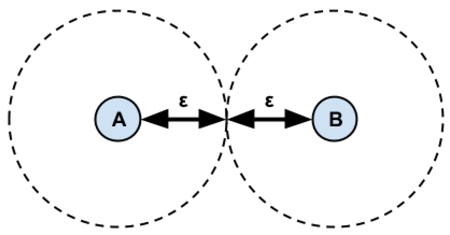
For two or more monitored individuals to be considered together in a group, there must be a minimum distance established between the points representing them. The algorithms proposed in this paper are functionally specified to consider this distance for processing geographical points in order to identify groupings of monitored convicts.

The minimum distance that characterizes a meeting, which is used as a threshold in the processing, must take into account the margin of error (ε) inherent to GPS equipment (Figure 2).

According to the National Satellite Test Bed/Wide Area Augmentation System (NSTB/WAAS) T&E Team [22], the accuracy of GPS devices is slightly smaller than 10 m. Thus, considering this margin of error, Equation (1) is applied to set the meeting distance threshold ($lr$). In other words, in practice, for calculation purposes, any two points separated by a distance under 20 m will be considered monitored subjects in proximity.

$$lr=2·|{\epsilon }_{min}|$$

(1)

3.1.2. Duration of a Possibly Detected Group

Detection of groups is performed considering not only the grouping of points in space at a given moment, but also the evolution of this group over time. Thus, indicators, such as group duration and average number of elements, are pieces of information that can be generated by comparing and identified groups in each sample points sent by the devices. Our proposed algorithms shall then provide for the processing of this information.

By maintaining a base of active and inactive groups updated at every sample processing, other information can be easily extracted such as the frequency and time that each group meets. This information supplements the analysis showing any real risk of imminent criminal action or a continued criminal relationship.

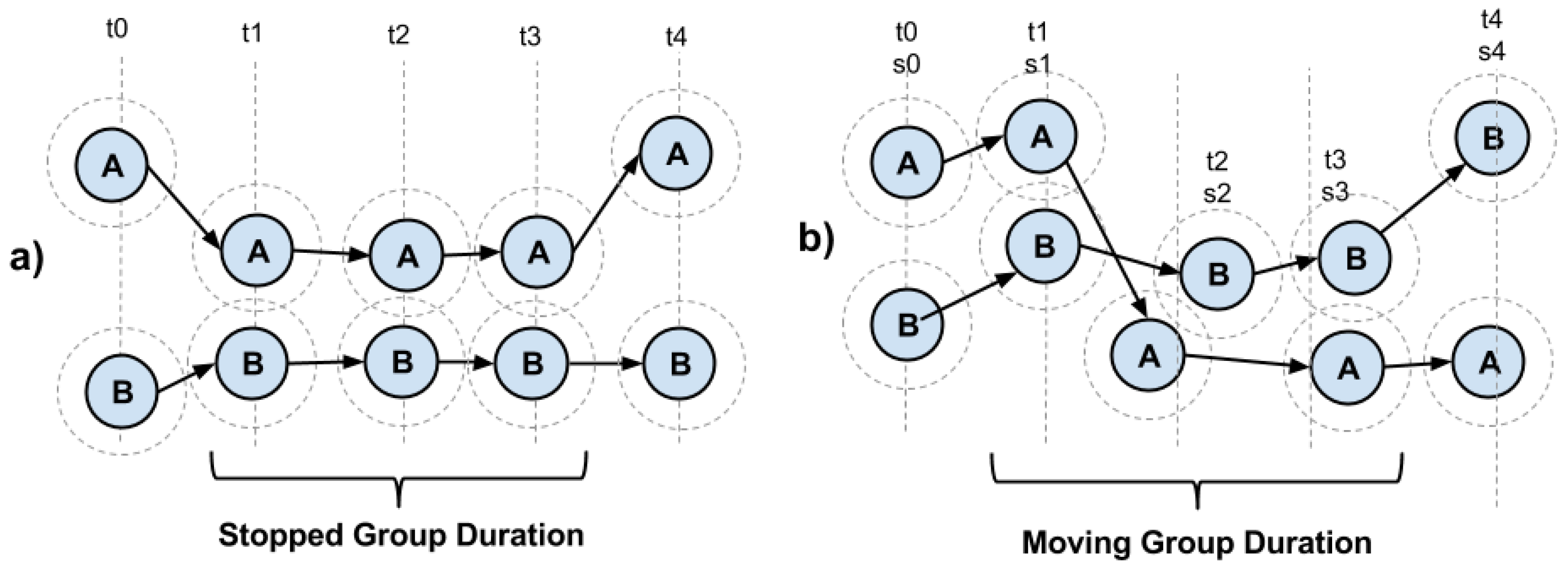
Figure 3a,b illustrates the measurement of group duration, respectively in situations where people are standing or moving. During the interval for computing points proximity, $t0$ is a specific time when there is not enough proximity between points to consider them as being grouped. At time $t1$, with the points coming close to each other, they are considered to be part of a group that at minimum has two member points. During the following processing times ($t2$ and $t3$), the same points still remain within the proximity range. At time $t4$, the two points separate from each other. The system will compute $t1$ as the start date and time of the group meeting and $t3$ the end of this meeting. Such data comprise the duration of the group existence. This same reasoning shall be applied both to stationary (Figure 3a) and mobile (Figure 3b) points in proximity.

When two monitored individuals intersect in some location, for instance an avenue, their physical proximity may be detected by these calculations, but it does not necessarily mean a grouping of monitored individuals. In order to avoid such situations defined as “false positive”, groups whose duration is less than a predetermined value should be discarded. Initially, this variable is set to a minimum of 5 min. In other words, considering minute to minute samples, when the same group is identified in the processing of five consecutive samples, those points in proximity will be considered as an effectively detected group.

3.1.3. Number of Elements in a Detected Group

The number of elements that are part of a grouping influences the evaluation of risk. For example, groups of five elements can pose a greater risk than groups of two elements, as this situation may represent a more severe and organized offense through the division of activities between group members. Hence, providing the number of individuals in a group at the end of the processing is important to support decision-making.

We should also consider that during the existence of a group, its number of individuals may increase or reduce, variations that can be detected by computing their proximity. These variations do not disqualify the group. Thus, we consider the average value of the number of individuals in the group during its existence, an indicator that allows us to consider proportionality in possible comparisons among groups.

However, a variation in the number members of a group can impact the comparison of this group with previously detected groups. This brings the question of how to accurately establish that a previously detected group that had, say, 10 individuals is for the most part the same as one that now has 12 elements: how many members the two groups have in common that yield the conclusion that one group is indeed a reduced or an expanded incarnation of the other. In order to consider this sort of recurrence of a group, we include in the routine that performs comparisons of groups a variable called “commonality”, which corresponds to the number of individuals common to both groups (current and former) divided by the total amount of former group elements, expressed as a percentage. If the commonality among two groups is equal to or greater than a commonality threshold, which is initially set to 50%, we consider that they are the same group, and in this case, an attribute containing the average amount of these group members is properly updated. Otherwise, the group under analysis is considered a new group to be remembered.

3.1.4. Time Limits for Running the Algorithms

Anklet devices are configured to periodically send their geographical coordinates or points, typically every 1 min approximately, although this time is usually configurable. Thus, the algorithms to identify groups and gather associated data must run in less time than this whole period boundary, i.e., before the next set of coordinates arrives for new calculation. Moreover, this limit is a performance threshold, because, if this limit is exceeded, there is a risk of accumulating tasks, or computing threads with the processing of the previous set, or overloading the equipment responsible for processing, or loosing information. Therefore, the whole algorithm must run in a time window that does not exceed the set of coordinates’ arrival period, which is set to 1 min in this paper.

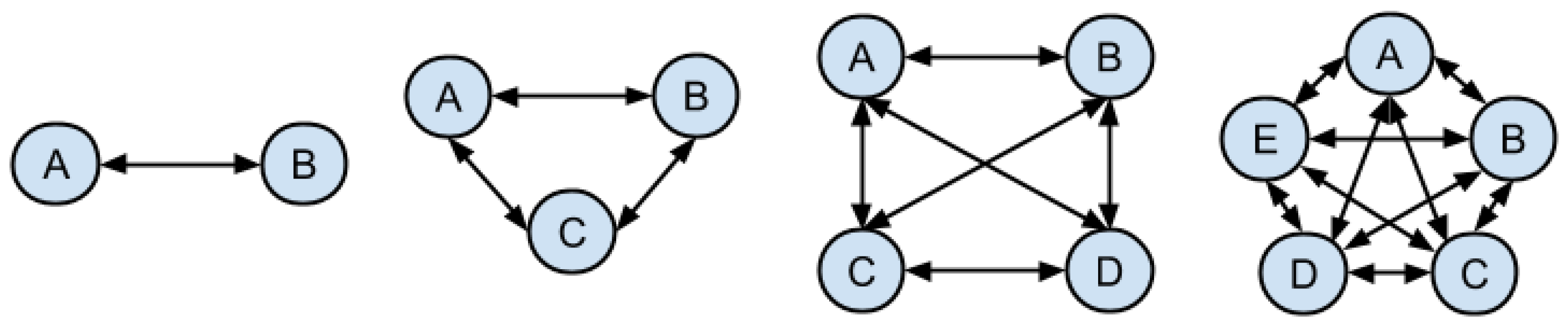
The algorithm is required to tackle a computational complexity problem related to the number of pairs of points to be treated, since we need to calculate the distance for each of these pairs, as shown in Figure 4. The distance from one point to the other in a pair of points allows evaluating if the two points are in proximity, a condition required to subsequently verify the points that are associated in groups. As the number of points belonging to a collected group increases, so does the number of comparisons necessary to identify these grouped points.

The number of comparisons for the verification of proximity is given by the simple combination formula (Equation (2)) where n is the number of items in a collection and p is the number of elements in each combination, so the result $C_{n,p}$ refers to the combination of n things taken k at a time without repetition. In our calculations, p is set to two since we refer to pairs of points in a sample of coordinates that must be treated each time.

$$C_{n,p}=\frac{n!}{p!(n-p)!}=\frac{n.(n-1).(n-2)!}{2.(n-2)}=\frac{n.(n-1)}{2}$$

(2)

For example, in a sample of 10,000 points, there would be approximately 50 million distance calculations. This number of computations and the required processing time window are critical factors for a successful implementation. Furthermore, it is important to control these factors since the amount of monitored individuals can grow with the evolution of an anklet-based monitoring system utilization, given the prison population growth rate, as shown in Figure 1.

The problem is solved partly by dividing the total coordinate space into subareas, which allows breaking down the processing instances, as described in Section 3.1.5. The proposed solution can be completed with the cooperation of parallel computing nodes. Indeed, to prevent the amount of monitored individuals from compromising the processing within a defined time window, the alternative proposal is an algorithm that processes subareas of the coordinate space in parallel. In this case, as the number of points to process grows, one can add more parallel nodes to the system for the completion of the processing within a required time window.

3.1.5. Division of the Coordinate Space into Subareas to Allow Processing Parallelization

The problem of executing a number of proximity-related computations within a required processing time window demands a solution where more computational power can be added to the system when the number of monitored individuals increases or when there is a reduction in the processing time window. Thus, the division of the coordinate area into smaller areas is proposed here so that the processing can be divided into several processing units.

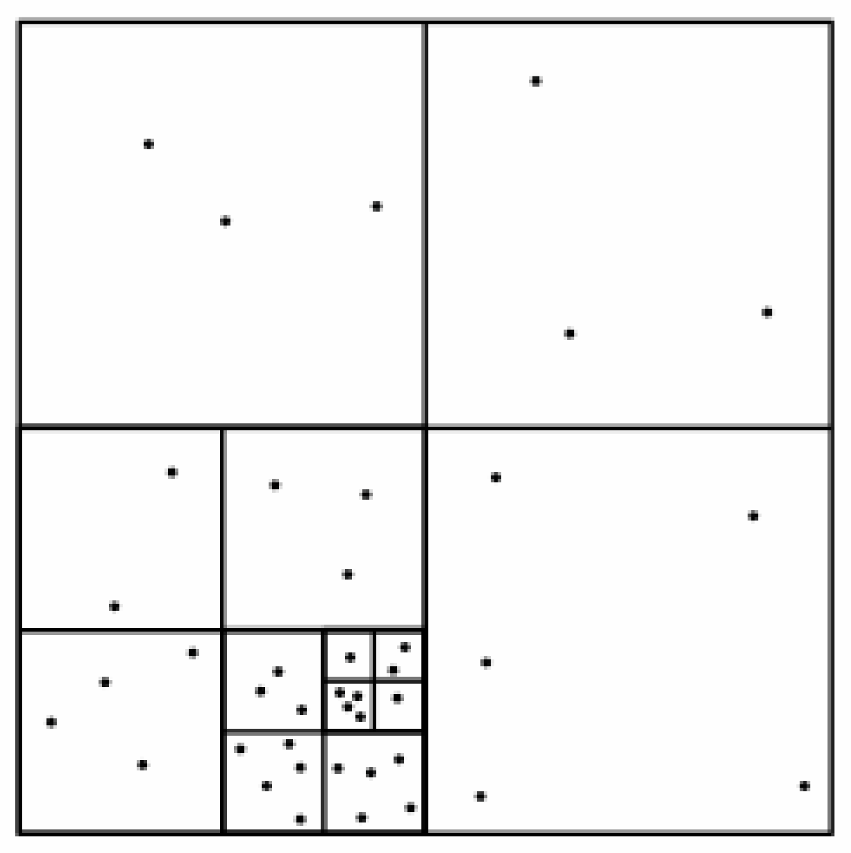
Referring to Figure 5, we consider an initial area computed from the farthest points in a periodical sample reported by the monitored devices. This constitutes the abstraction of a square geographical area containing all of the sample points. Then, a recursive division of this area takes place guided by a divide-and-conquer strategy as follows, also supported by the work from Ding and Densham [21].

First, the abstracted area is divided into four smaller areas of equal size (quadrants), and the number of points in each quadrant is counted. If it is observed that a quadrant contains more points than a quadrant population threshold, this quadrant will be further divided so that the recursive quadrant divisions result in a number of quadrants, each one containing a number of points that do not represent a performance processing problem regarding proximity calculations within the limited time window. The quadrant population threshold, i.e., the maximum amount of points a quadrant can have, is arbitrarily fixed in this paper, but as this threshold is bound to the available processing capacity, it should be considered as a variable whose behavior is a matter of future study. Furthermore, a quadrant cannot be subdivided if the length of its size is less than the proximity distance threshold.

This recursive subdivision of the original space is similar to that proposed by Xia et al. [23] using a quadtree structure. However, this study does not consider the hierarchical link between subareas. The central interest is that each of these areas can be processed independently from the other areas, which enables processing parallelization. In another alternative view, the distance calculations occur only inside the quadrants where the points are, thus reducing processing effort. However, although we no longer compare points that are from distant quadrants and thus reduce the number of distance calculations, there will be situations where two points are in proximity in adjacent quadrants, and there is a possible identification failure for that pair. 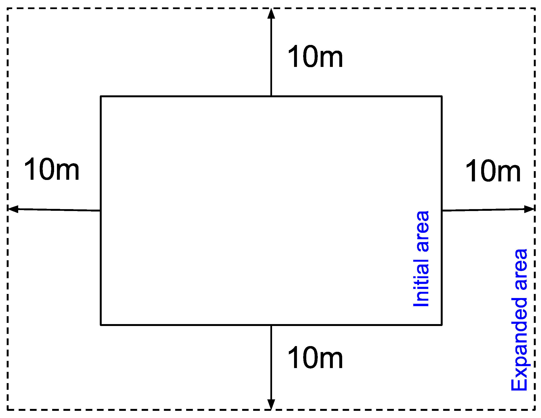Referring to Ding and Densham [21], we have an alternative to solve this problem, by expanding the area of a newly-created quadrant (Figure 5) by adding to it a margin equivalent to the minimum distance for identifying points in proximity (Figure 6).

Considering this added margin, each area overlaps the adjacent ones, allowing proximity calculations for points that are close to points in adjacent quadrant borders. Since the calculations for a quadrant are independent of those for another quadrant, it is possible to obtain duplicate responses for the same pair of points in proximity (A-B and B-A). Such duplication does not pose a problem as duplicates are eliminated by the groups detection algorithm explained in Section 3.2.4 and shown as Step 3 of the systemic model (Figure 7).

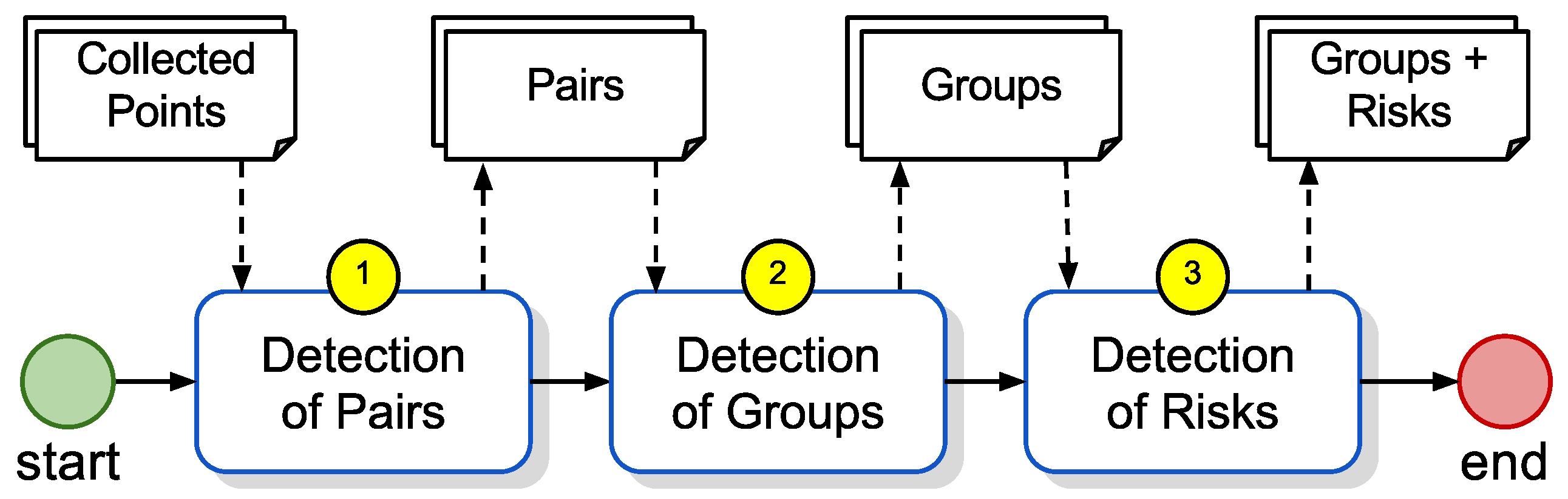
3.2. Systemic Model and Associated Algorithms

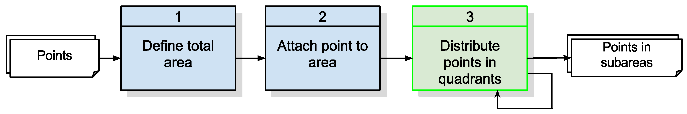
Figure 7 shows the systemic model proposed in this paper, which divides the processing into three steps: (1) detection of pairs: receive a collection of points sent by the devices through the network, and calculate the points in proximity; (2) detection of groups: group the points in proximity in clusters; and (3) detection of risk indicators: add data on group duration and the number of participants.

The first step receives as input a collection of points collected at a given instant (collected points), whose structure is described in

Table 1. Collected points: Algorithm 1 (detection of pairs) input.

Attribute	Type	Description
Device	Integer	Device identifier number
Date/time	Date/time	Date, hour and minute when the point was collected
Point	Geographic coordinate	Geographic point consisting of latitude and longitude

. The collected points are treated in the second step by the detection of pairs algorithm, which generates a list of points in proximity (Table 1). Subsequently, the detection of groups algorithm examines in Step 2 the list of pairs and generates a list of identified groups whose risk attributes are then calculated in Step 3, resulting in the final output structured as specified in

Table 2. Groups and risks: Algorithm 3 (detection of risks) output.

Attribute	Type	Description
Group	Integer	Uniquely identifies the group
Start Date/time	Date/time	Date/time when the group convenes
End date/time	Date/time	Date/time the group dispersed
Processing turn	Integer	Number of processing turns in which the group was detected
Devices quantity	Integer	Cumulated sum of the number of group elements used for calculating the average number of group members
List of devices	List of device identifier numbers	List of devices that have been members of the group

.

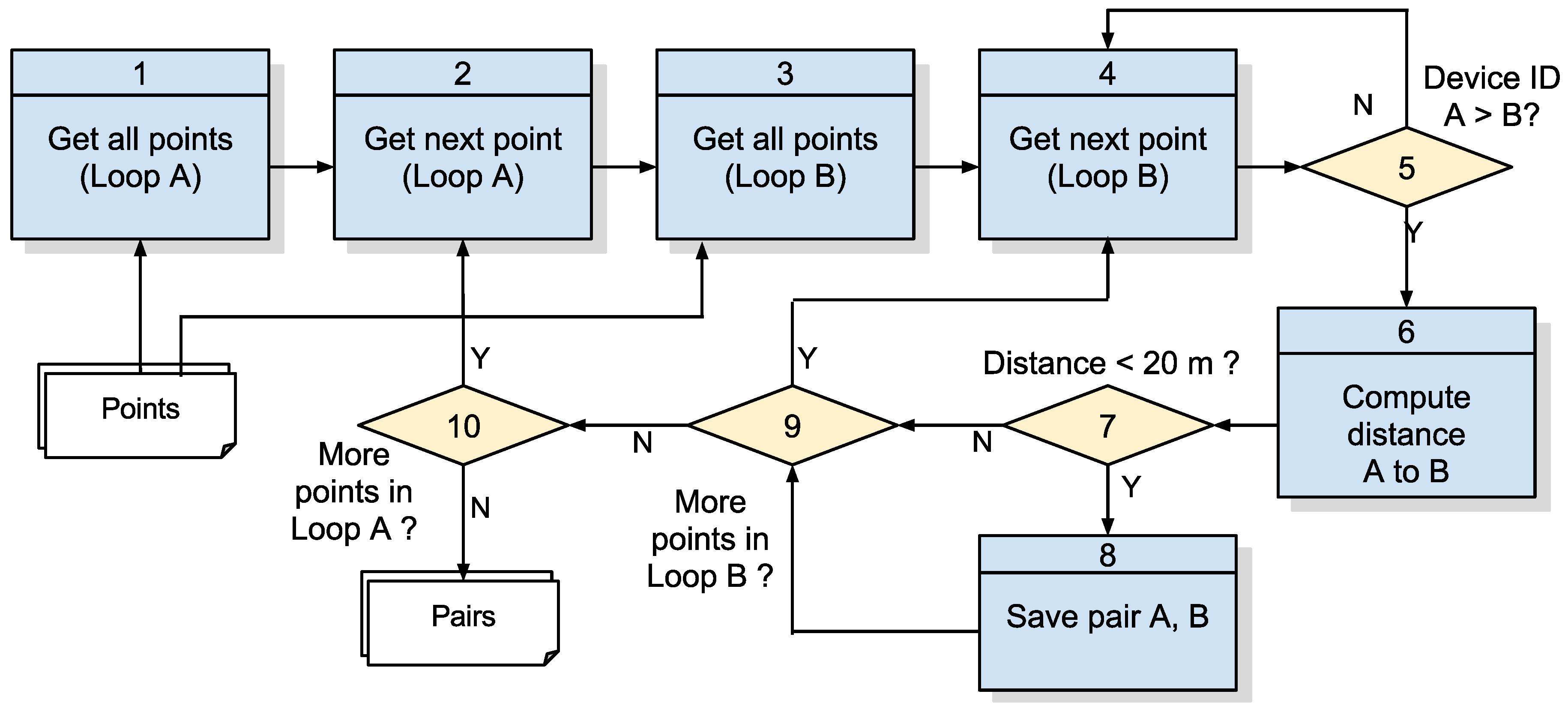
3.2.1. Algorithm 1: Detection of Pairs

Referring to Figure 8, detailing Step 1 of Figure 7, the coordinate points are compared to each other, and the pairs whose distance is less than or equal to $lr$ (Equation (1)) are identified as pairs of points in proximity and added to a list that will be part of the output of the algorithm. In this case, it it worth remembering the distance considered for this approach is 20 m due to precision errors that occur in GPS systems as detailed in [22]. Its input is a list of points collected with the structure detailed in Table 1, and its steps are detailed in

Table 3. Detailed steps of Algorithm 1 (detection of pairs).

#	Description
1	Since it is necessary to compare the points to each other, the process starts a loop considering all collected points.
2	It takes each point obtained in the previous item relative to Loop A.
3	It sweeps again all collected points (Loop B) to be compared with Loop A points.
4	It takes each point obtained in the previous item relative to Loop B.
5	This filter prevents the calculation of the distance from A to B to be repeated for B to A. If A is greater than B, it ignores this pair and goes back to Step 4.
6	It uses a geoprocessing function and obtains the distance from A to B in meters.
7	If the distance is greater than $lr$ meters, then Points A and B are not in proximity, and the flow proceeds to the next point to be used in Loop B.
8	If Points A and B are at $lr$ meters or less away from each other, then they are considered to be in proximity and are recorded/stored for the grouping step.
9	If there are more points relative to Loop B to be compared, then it diverts the flow to capture the next Point B.
10	If there are more points relative to Loop A to be compared, then it diverts the flow to capture next Point A. If there are no more points, the comparison processing is completed, and as a result, it outputs records with pairs of devices in proximity.

.

This step is the most costly in computational terms, as it implies the comparison between all of the points in the sample to identify points in proximity (Figure 4).

3.2.2. Algorithm 1.1: Recursive Division of the Original Space into Subareas

Given the concepts presented on the definition of proximity and the idea of dividing the space into smaller quadrants as a function of the number of points to be treated, we have devised the algorithm shown in Figure 9, which is responsible for receiving the collected points, then defining the adequate quadrants and listing the points that are inside these quadrants (Figure 5).

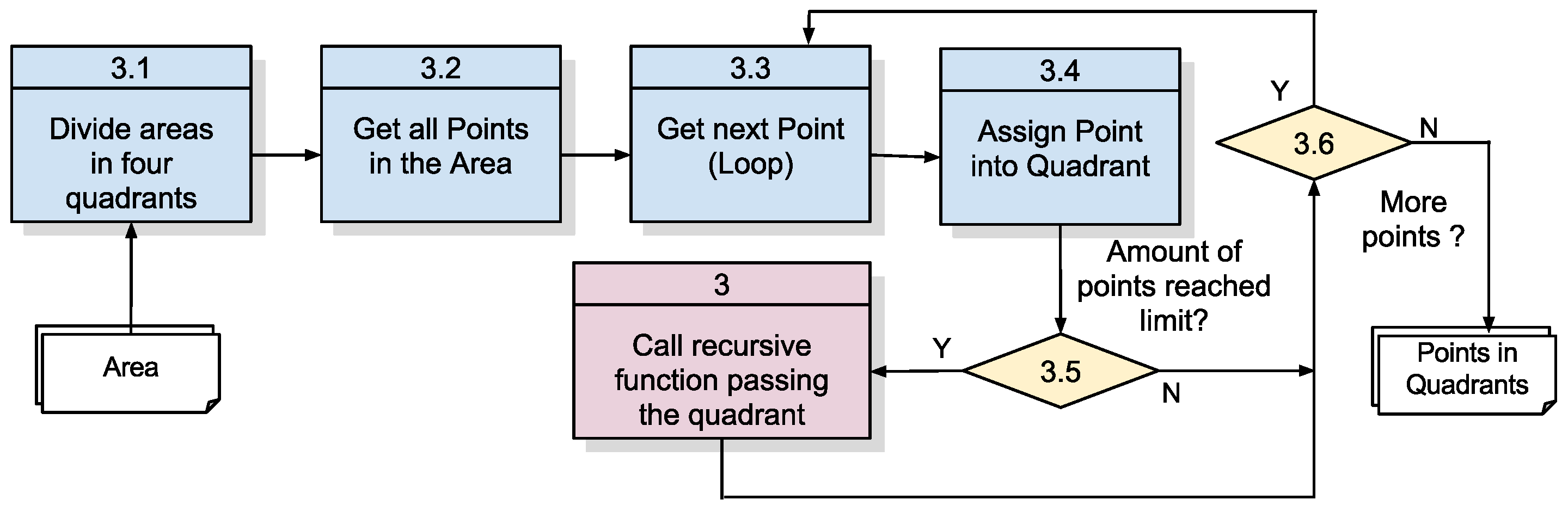
The first two functions define an initial area covering all collected points and links all points to this initial area. This is necessary so that Function 3 can work recursively. Function 3 always receives an area with its points and then makes a decision whether it is necessary to subdivide this area into smaller quadrants. The decision criterion stipulates that if the number of points inside the area exceeds the quadrant population threshold, this area must be subdivided into smaller areas that will be recursively submitted to Function 3. The details of this algorithm are specified in

Table 4. Detailed steps of Algorithm 1.1: division into subareas.

#	Description
1	It obtains the most distant points of the map and generates a square geographical area that covers all points to be processed.
2	It links the points to be processed to the area created in the previous item. This step is required as a preparation for the first call to the recursive function described in the next item. The input parameter for this function is the area with its collection of points.
3	The recursive function divides the received area into quadrants (four new areas) and modifies the links of the points from the received area to the new quadrants according to the coordinates of these points.

.

The recursive function shown in Figure 9 has its algorithm shown in Figure 10, while

Table 5. Steps of the recursive space division function in Algorithm 1.1.

#	Description
3.1	The area received as input is divided into four quadrants. Recursively, this division is performed for the initial processing of the total area or when one of the quadrants has a number of points that exceeds the quadrant population threshold. Each created quadrant has its area expanded to contemplate proximity among points that are close to each other, but pertain to different adjacent quadrants.
3.2	It reads all of the points that are linked to the area provided as input, preparing then to move each of the new quadrants according to their coordinates.
3.3	With the points supplied in the previous item, a finite loop is run to assign the appropriate treatment.
3.4	According to the coordinate of the point, it is copied from the input area to the corresponding quadrants. Due to the area expansion of each quadrant performed in 3.1, a point may appear in more than one quadrant.
3.5	During the loop, if the number of points linked to a quadrant reaches a maximum value, this quadrant is used as input for a recursive call to further divide this quadrant.
3.6	If there are still points to be treated, the loop is repeated for the next point.

describes the steps of this recursive function.

Each subarea set of points can be assigned to be processed on different computational nodes, which allows the work to be parallelized. While on the one hand, we ensure that each subarea has a number of points smaller than an established threshold, on the other hand, we may have subareas with a small number of points. This may represent a potential waste of computing and memory resources since the processing varies according to the number of points in the subareas. However, a scheduling process was adopted in this work that distributes sequentially the subareas in the available threads, minimizing possible differences in the total processing time in the nodes.

Algorithm 1.1 generates a list of points with their respective subareas to be processed in parallel by Algorithm 1.2. Such a structure is detailed in

Table 6. Groups and risks: Algorithm 3 (detection of risks) output.

Attribute	Type	Description
Device	Integer	Device identifier number
Date/time	Date/time	Date, hour and minute of point collection
Point	Geographic coordinate	Geographic point consisting of latitude and longitude
Subarea	Integer	Identifier of the subarea containing the point

.

3.2.3. Algorithm 1.2: Detection of Pairs within Subareas

The algorithm for the detection of pairs within subareas is the same described in Figure 8, only differing on the list of points to be processed. The output of this algorithm is a list containing pairs of points in proximity whose structure is detailed in

Table 7. Algorithm 1.2 output structure (detection of proximity pairs).

Attribute	Type	Description
Pair	Integer	Pair identifier number
Date/time	Date/time	Date, hour and minute of point collection
Device A	Integer	Device identifier number
Point A	Geographic coordinate
Device B	Integer	Device identifier number
Point B	Geographic coordinate	Geographic latitude and longitude of the point

.

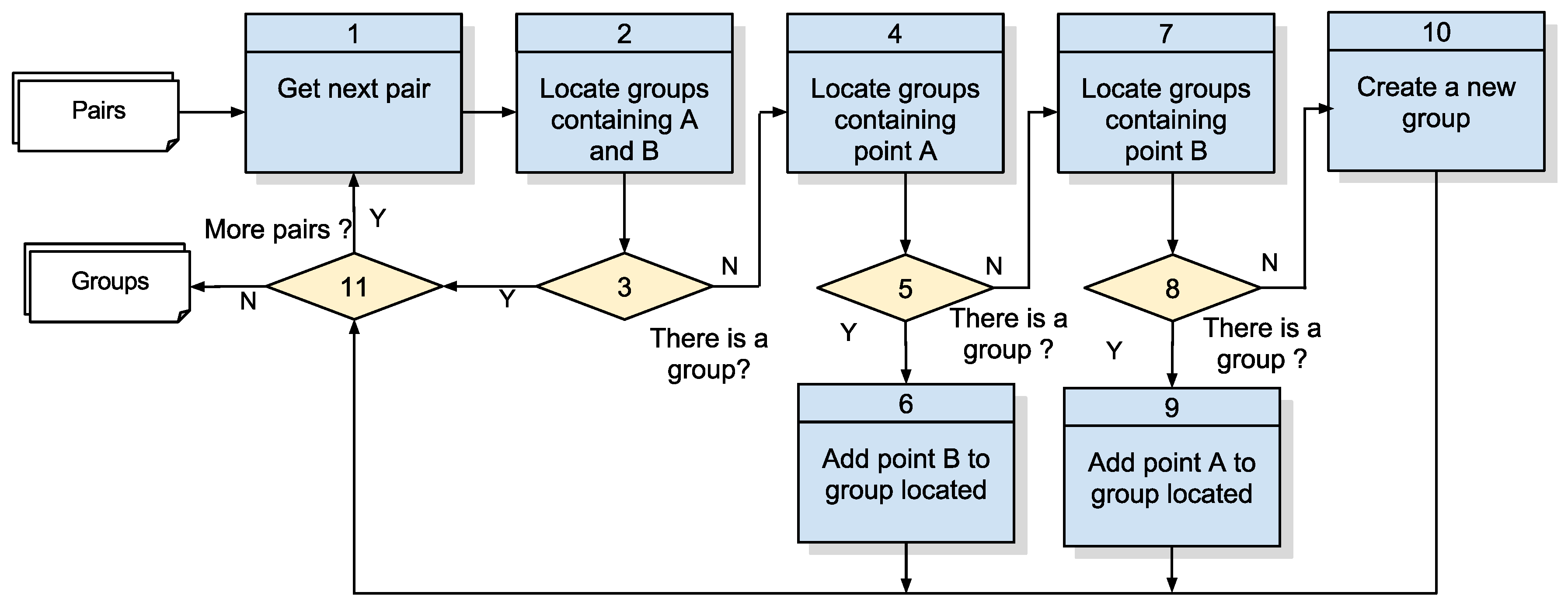
3.2.4. Algorithm 2: Detection of Groups

This algorithm, Number 2 of Figure 7, takes the pairs of points considered in proximity by Algorithm 1.2 and then finds those that are grouped by looking for neighbors of a neighbor, i.e., in situations where Point A is close to B and Point B is close to C; hence, A, B and C form a group of monitored individuals. This detection of groups algorithm is presented in Figure 11, while its details are specified in

Table 8. Detailed steps of Algorithm 1 (detection of pairs).

#	Description
1	It obtains each pair, A and B points, of the set obtained in the previous step.
2	It checks for any group from previous iterations that already has Points A and B and eliminates any possible repetition.
3	If a group with the 2 points is identified, then nothing needs to be done, and the loop must continue to the next pair.
4	It checks for any group that has at least Point A.
5	If the group is located, then it does not have Point B.
6	It adds Point B to the group located in the previous item.
7	It checks for any group that has at least Point B.
8	If the group is located, then it does not have Point A.
9	It adds Point A to the group located in the previous item.
10	If no group is located containing either A or B, then a new group must be created with the A and B pair. This group can then be completed as new points are discovered in later iterations.
11	If there is still a pair to be processed, then it processes the next pair; else the algorithm ends.

and its output in

Table 9. Algorithm 2 output structure (detection of groups).

Attribute	Type	Description
Group	Integer	Group identifier number
Date/time	Date/time	Date, hour and minute of point collection
Device list	Integer list	List of devices that make up the group

with a list of groups, each one having an identifier, a timestamp for the moment the points were collected and a list of devices composing the group.

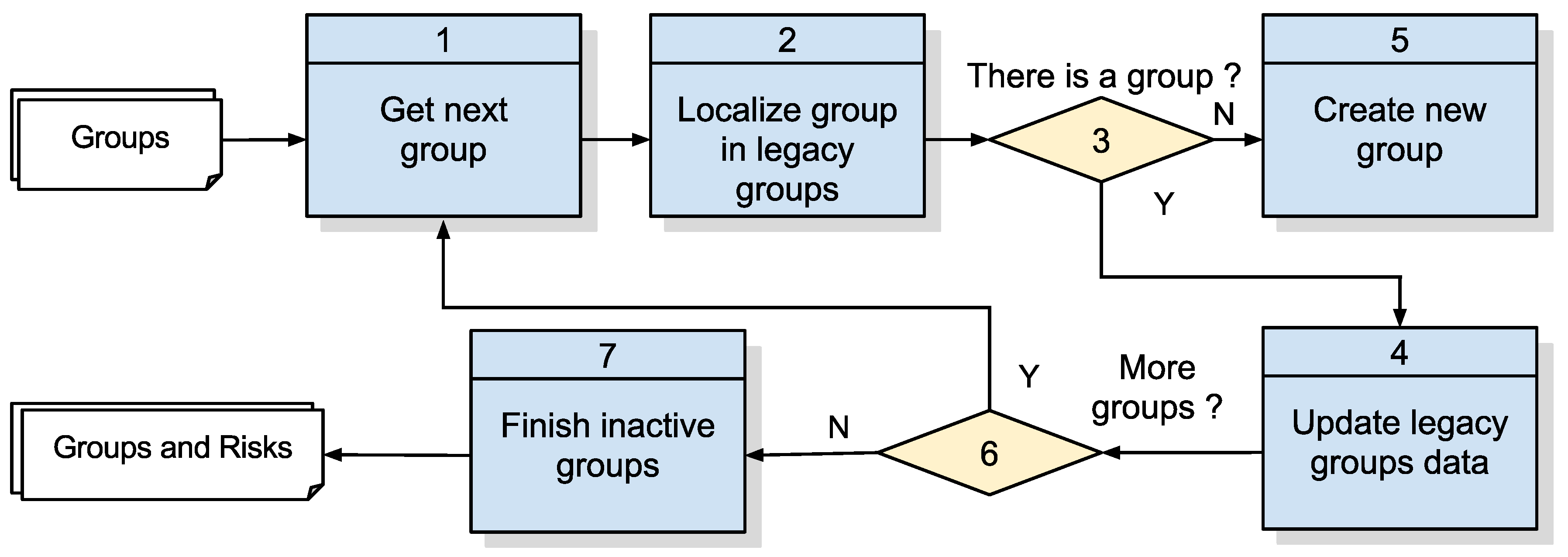
3.2.5. Algorithm 3: Computation of Risk Indicators

Detection of risks, which corresponds to Algorithm 3 in Figure 7, computes for a group of monitored individuals additional data regarding the duration of the group and the average number of elements, indicators that are updated as new samples are collected from monitored devices. From the standpoint of anklet monitoring, these data about groups may contribute to the risk analysis to be conducted subsequently to performing the specified algorithms. The proposed solution in this paper just computes the risk indicators linked to identified groups and stores these data for a risk analysis activity to be performed outside the monitoring system.

During its execution (Figure 12 and

Table 10. Algorithm 3 specification (group risk indicators).

#	Description
1	It obtains each group detected in the current processing turn.
2	In the set of previous active groups, it identifies the groups that possess at least 50% of its members in common with a group detected in this processing turn. The 50% percentage parameter is an arbitrary choice to be further investigated in future studies.
3	If no compatible group is found, then the flow is directed for the creation of a new group in Item 5.
4	It updates the number of processing turns for the group and adds up the number of elements counted in each processing turn. These two attributes provide the necessary data for averaging the number of members of the group during its existence.
5	It creates a new group considering the processing count attribute as 1, the start date/time attribute as the timestamp of the current processing and the elements count attribute as the respective number of group members.
6	If there are more groups to be processed, then it directs the flow to capture the next group; else it then closes the existing groups, as per Step 7.
7	Existing groups that were not identified in the current processing turn should be ended. This is done by updating the group’s end date/time with the value corresponding to the immediately previous processing turn, i.e., the last time the group was detected. As a result of the processing, a set of groups is generated, as well as their duration and number of members for utilization in the next processing turn.

), Algorithm 3 collects the following data: (i) group duration: this indicator comes from the perception that groups that last longer may be indicative of greater risk and even that groups with a very short duration may be discarded; (ii) the average number of elements in each group: groups with a higher number of elements can indicate larger scale violations involving, for example organized crime or conspiracy.

In order to indicate the duration or permanence of a group, the algorithm must update this previously identified group with data regarding duration (start/end date/time). When the end date/time attribute is not populated, it indicates that the group is still active, i.e., it has been continuously sustained until the last data fusion execution. Registered dates/hours for the group do not represent the exact instant of this group start or end, as they are influenced by wait and service times during sensor data collection and the execution of the algorithms themselves.

As discussed before, the output of Algorithm 3 is specified in Table 2. The resulting structure is then available for risk analysis and for future processing turns.

4. Validation Scenarios and Results

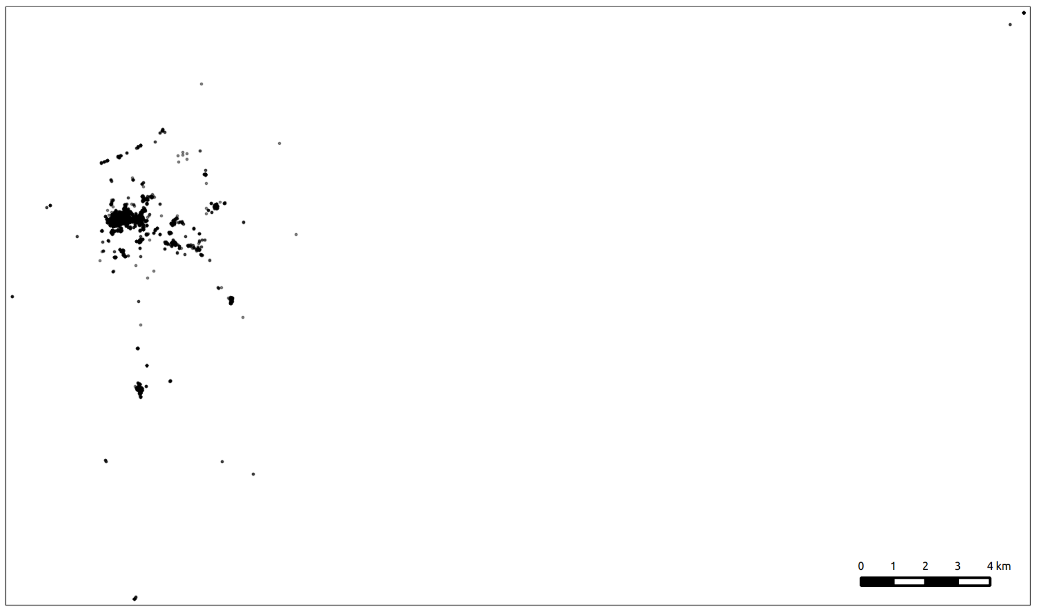
In order to validate the algorithms presented in this paper, a simulated database was used with approximately 10,000 devices. The simulation of groups was performed by creating variations of a set of paths obtained from real GPS equipment. The simulated new routes were composed using the horizontal and vertical displacement of the original device coordinate points in the geographic space, also increasing the number of coordinate points in the sample. Moreover, new routes were created by reversing the latitudes and longitudes and attributing them to new simulated points. As a result, three sets with 10,000 points each were generated. These samples correspond to three consecutive collections of points from simulated anklets in a simulated schedule, respectively corresponding to the date 25 May 2015 at time tags: (i) 12:00, (ii) 12:01 and (iii) 12:02. In

Table 11. Sampling extracted from simulated database.

Timestamp	Device ID	Latitude	Longitude
25 May 2015 12:00:00–03	12133	−29.903980255127	−51.169883728027
25 May 2015 12:00:00–03	1096	−30.062665939331	−51.192127227783
25 May 2015 12:00:00–03	41978	−29.778089523315	−51.108917236328
25 May 2015 12:00:00–03	817	−30.028823852539	−51.225776672363
25 May 2015 12:00:00–03	40413	−30.093103408813	−51.177989959717
...	...	...	...
25 May 2015 12:01:00–03	12123	−30.087636947632	−51.231784820557
25 May 2015 12:01:00–03	10871	−30.049358333333	−51.162086666667
25 May 2015 12:01:00–03	1969	−30.114995956421	−51.362251281738
25 May 2015 12:01:00–03	91523	−29.70588684082	−53.802436828613
25 May 2015 12:01:00–03	91042	−30.050704956055	−51.21089553833
...	...	...	...
25 May 2015 12:02:00–03	5575	−30.016288757324	−51.11653137207
25 May 2015 12:02:00–03	11716	−30.062965393066	−51.142623901367
25 May 2015 12:02:00–03	12165	−30.201919555664	−51.134094238281
25 May 2015 12:02:00–03	5954	−29.986715316772	−51.1682472229
25 May 2015 12:02:00–03	1047	−30.086135864258	−51.234657287598
...	...	...	...

, there is a sampling of records randomly extracted from the simulated database.

As an example of a coverage area, the 10,000 points regarding Timestamp 25 May 2015 12:00:00-03 sampling are spread in a geographic area as illustrated in Figure 13.

The computing configuration used to validate the proposed algorithms execution is presented in

Table 12. Equipment used in tests.

Resource	Specification
Processor	Core i5-2467M 1.6 GHz (dual core with hyper-threading)
Memory	8 Gigabytes
Hard drive	516 Gigabytes 5400 RPM hard disk
Operating system	Ubuntu 14.04.4
DBMS	PostgreSQL 9.4

.

The proposed algorithms are implemented and evaluated in five scenarios. The first one is a serial implementation in a relational database query language (scenario). This classical scenario for application development is taken as a baseline for comparing the results in this paper since it does not deploy any particular performance contribution, though it presents the complete correct functionality proposed in this paper. The other scenarios gradually present the contributions of parallelism (Scenario 2) and programming language (Scenarios 3 and 4) for the proposed algorithms, maintaining the same functionality. The possible distributed processing scenario is analyzed in the discussion of the results.

Specifically, for correction purposes, in all evaluated scenarios, the number of records resulting from the execution of each algorithm applied to the simulated data is given in

Table 13. Results of the algorithms’ processing.

Algorithms	Collection of Points
	12:00	12:01	12:02
Number of Subareas	22	37	91
Detection of Pairs	9103	9580	14,686
Detection of Groups	1673	1762	1854
Detection of Risks Indicators	406 active groups in all collections

.

In the presentation of each scenario’s results hereafter, measurement values are the average of 10 repeated executions.

4.1. Scenario 1: Serial Processing in PL/pgSQL

In this scenario, the described Algorithms 1–3 are fully executed in serial processing, and the performance of each one is measured. Each of the three algorithms is measured separately, and then, their summed response time is presented. This method is chosen to enable reasonable comparisons with results from subsequent scenarios, when parts of those algorithms are replaced by modules in parallel processing or in C language or in distributed processing.

4.1.1. Algorithm 1: Detection of Pairs

The implementation is of a simple algorithm that compares all of the coordinate points by obtaining a list of pairs of points in proximity generated via a SQL statement that performs a self-join on the table of points. In this SQL command, a filter in the where clause selects only the points whose calculated distance is less than the proximity threshold. This threshold was defined at 20 m as stated in Section 3.1.1. Furthermore, in this where clause, a filter is added that considers only the points where the ID of a point A is smaller than the ID of a point B. This filter prevents calculating two times the distances between the same pair, i.e., distance from A to B and from B to A, thus reducing processing effort. As output, a table of pairs is generated. For instance, the output table, corresponding to our sample tagged 25 May 2015 12:00, has an approximate number of 9103 records (pairs of points in proximity).

This algorithm was tested with distance varying 10, 20 and 40 m as the threshold. Though there was variation on the amount of pairs detected because of the distance variable, the response time remained approximate. Besides, 20 m is acceptable within the error precision [22].

4.1.2. Algorithm 2: Detection of Groups

In order to identify groups of points in proximity, the developed the PL/pgSQL code specified in Figure 11 generates a table of groups with 1673 identified groups.

4.1.3. Algorithm 3: Computation of Risk Indicators

This algorithm is a PL/pgSQL module according to Figure 12. However, the implementation language allows a code improvement by applying an update on the set of records that meet the filter instead of checking each group obtained in the recent processing against each of the previously detected groups.

4.1.4. Response Time Results

Notably, the algorithm that detects pairs of points in proximity presents a much higher processing time than Algorithms 2 and 3, reaching an average time of 280 s (Figure 14). When considering the required overall performance threshold (fixed to a 1-min processing window), the sum of times from the three processing algorithms exceeds this value, which forewarns of their impracticality. However, the measured values are interesting as a baseline for the subsequent validation scenarios.

Scenario 1’s results illustrate the response time issue when identifying coordinate points in proximity without the use of parallel processing, which justifies the next scenario.

4.2. Scenario 2: PL/pgSQL Processing with Multiple Parallel Instances

In Scenario 1, the Algorithm 1 for the detection of pairs, which takes much more time than the other two algorithms, is the observable candidate for improvement, thus being reformulated in Scenario 2 by adding an inner algorithm to distribute points into subareas (Algorithm 1.1), which allows the identification of pairs (Algorithm 1.2) to be executed in multiple parallel instances. As Algorithms 2 and 3 are not modified from Scenario 1, they are not presented in Scenario 2.

The division of the whole coordinate space into smaller quadrants implies the corresponding division of the number of coordinate points to be compared in each quadrant processing. Now, there is a trade-off regarding the number of points that is used as a decision criterion for recursive sub-divisions of quadrants. It is necessary to set the maximum amount of points per quadrant subarea, considering that the smaller this number, the greater the number of subareas.

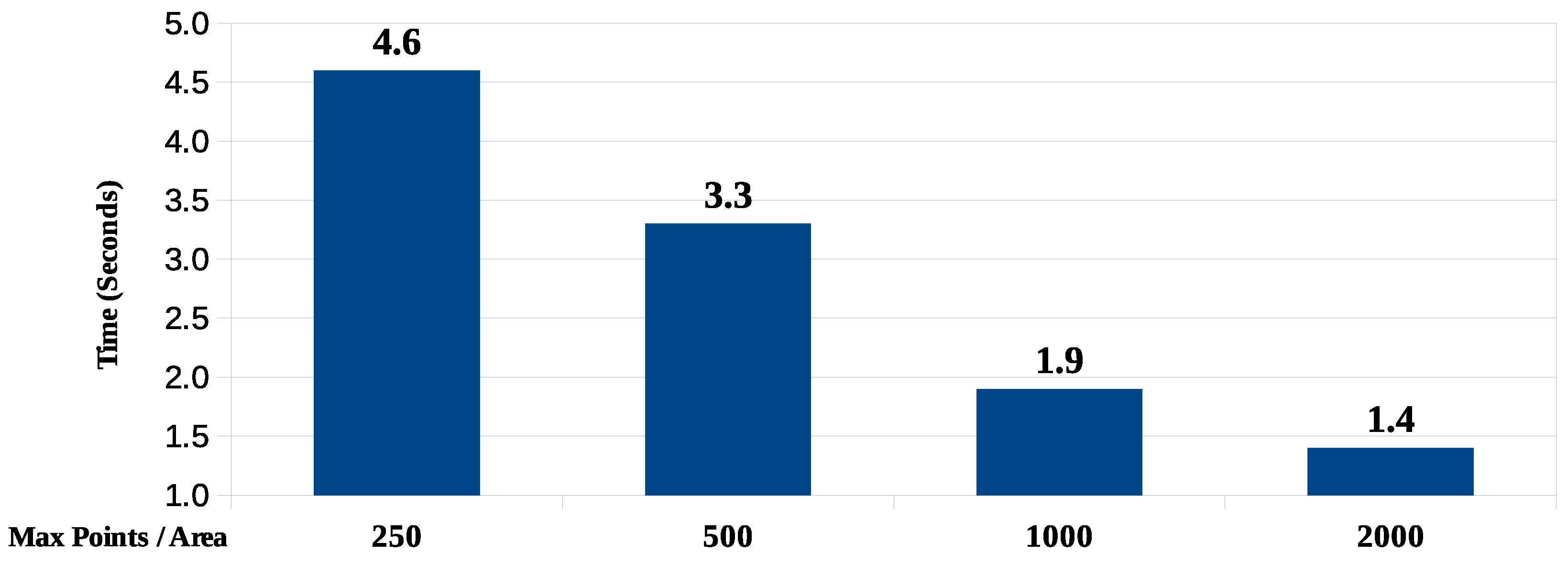
Given that we have established a database of 10,000 coordinate points for all validation scenarios, we define four cases for the maximum number of points per subareas (respectively 250, 500, 1000 and 2000) and obtain response time figures for these cases.

4.2.1. Algorithm 1.1: Distribution of Points per Subareas

This algorithm, implemented in PL/pgSQL according to the flows in Figure 9 and Figure 10, based on 10 repeated executions, presents the average response time results shown in Figure 15, for each of the maximum values of points per subarea.

Data concerning the sub-divisions of the coordinate area are presented in

Table 14. Maximum points per area and area size.

	Max Points per Area
	2000	1000	500	250
Number of Subareas	22	37	91	151
Average Area Size (m2)	6,662,905.40	3,961,789.13	1,610,986.67	970,874.14
Smallest Area Size (m2)	9023.61	2275.65	578.85	149.74
Largest Area Size (m2)	36,643,506.10	36,643,506.10	36,643,506.10	36,643,506.10

. As expected, the larger the maximum number of points per area, the less is the average area size to be processed. The size of the largest area is always the same since it corresponds to the first subdivision of the total area corresponding to 146.56 km${}^2$.

The lesser the maximum amount of points per subarea, the smaller the average size of the subareas. The size of the smallest area resulting from the most recursive division into quadrants also decreases with the number of points per area. In the smallest of the cases, the resulting subarea is approximately 150 square meters wide.

4.2.2. Algorithm 1.2: Detection of Pairs with Multiple Parallel Instances

The pair detection algorithm from Scenario 1 is adapted to run in parallel. Since PostgreSQL does not support developing routines in PL/pgSQL, we use a shell script running under an Ubuntu operating system that concurrently submits different instances of the same routine so that each instance considers a group of distinct areas.

4.2.3. Response Time Results

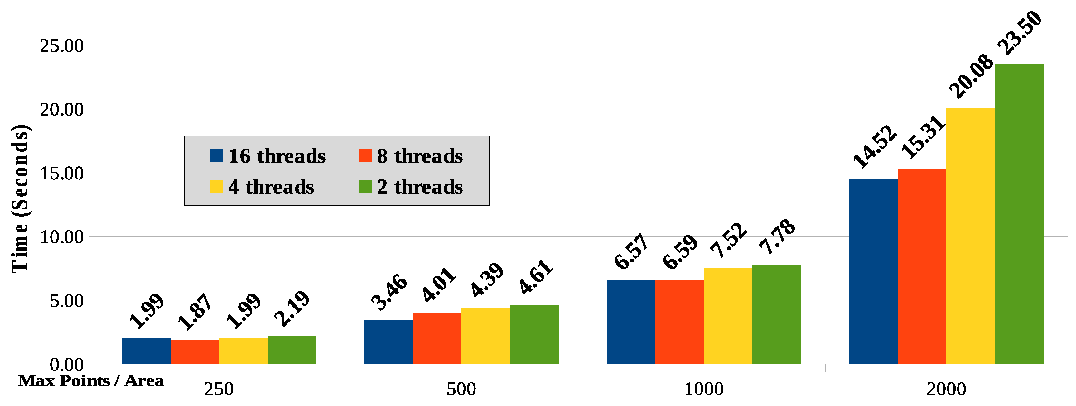
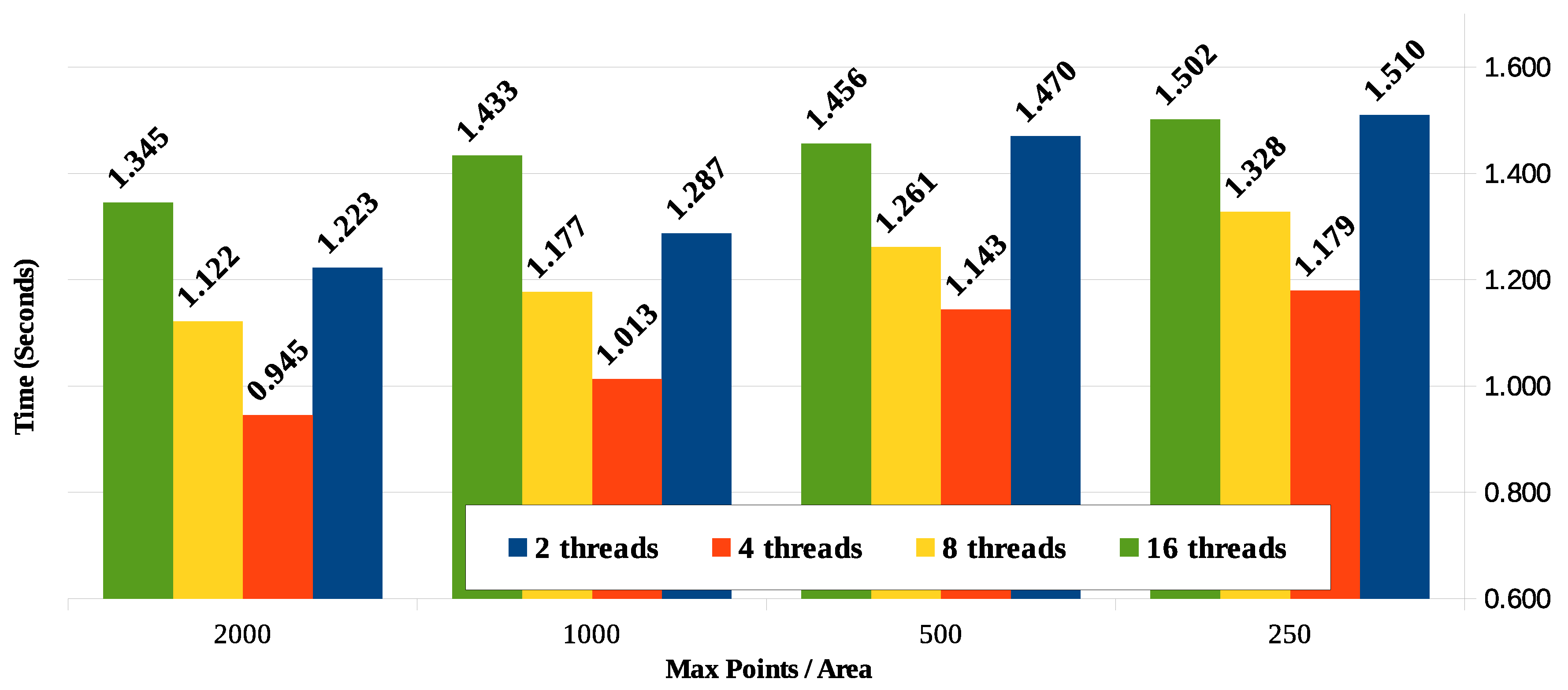
Figure 16 shown the compared response time results for the parallel processing taking into account the four values for the maximum points per coordinate subarea (250, 500, 1000 and 2000) and the number of processing threads used (2, 4, 8 and 16).

The amount of subareas will typically be greater than the number of computing nodes (or cores) available to handle them. Despite knowing that it is not the best technique due to variation in the amount of points per subarea (zero to the max points per area), we assume in this paper that the distribution of subareas among the computing nodes will be applied in stages, similarly to a round-robin algorithm. This can result in an overload of specific nodes while others become idle. A better distribution processing technique between nodes is a subject for further work.

Figure 16 shows that as the maximum number of points per area is reduced, so is reduced the corresponding processing time due to the lower number of comparisons between points necessary for processing and calculating the distance. For the sample used in this work and considering the results in Scenario 1, the response time reduction is significant and tends to flatten with the reduction of points per subarea.

The equipment used has processors with two cores and hyper-threading technology that simulates four logical cores. It was expected that the best response time would be with four threads. However, for areas with a higher number of points (1000 and 2000), the cases with eight and 16 threads showed better results. For areas defined with less points, the difference regarding the number of threads is smaller. It should be taken into account that, as the processing performs some disk read and write operations, the consequent I/O wait time seems to explain the better response time when processing with more threads.

4.3. Scenario 3: Algorithm 1.2 in C Language without Parallel Processing

In this scenario, for comparison, a routine was developed using the C language for implementing the algorithm for the detection of pairs (Figure 9) without parallel processing. All points are compared with the others identifying those who are in proximity by calculating the respective distance. In this case, there is no division of points into subareas, and the entire process is performed serially. The routine reads the 10,000 points from a file in a file system and writes the result as a text file in the same file system.

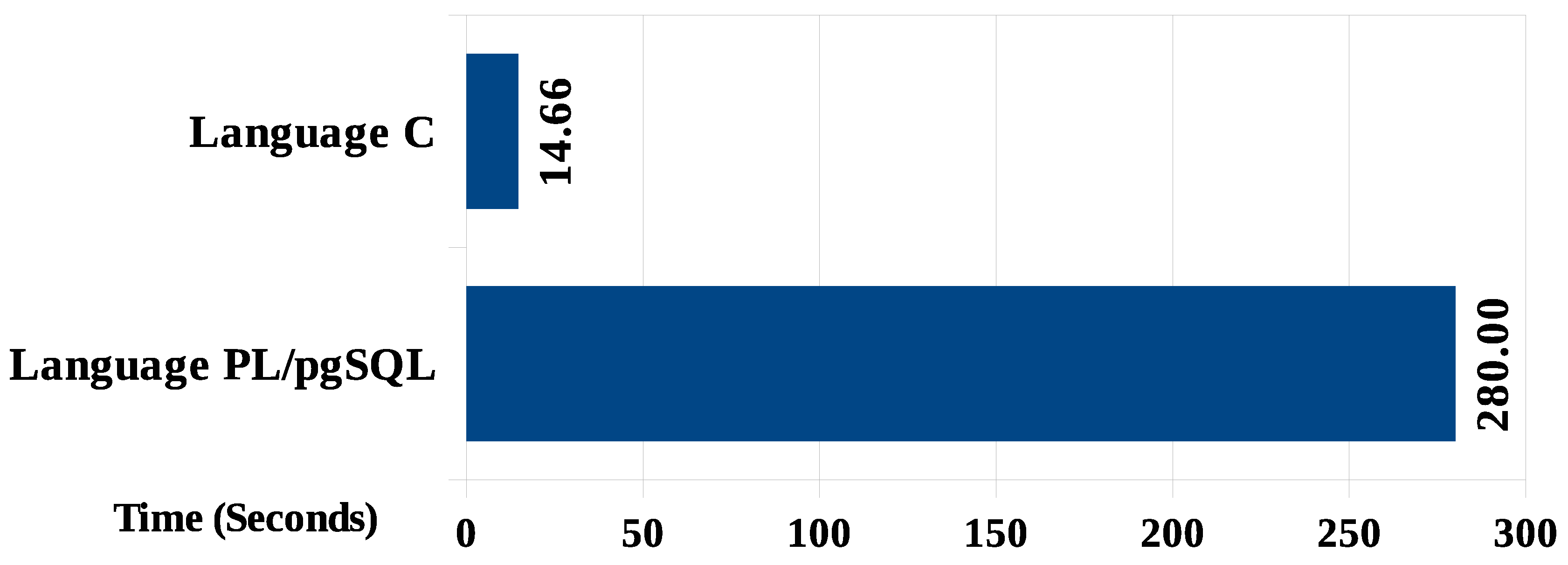
The processing response time (Figure 17) for Algorithm 1.2 in C language was approximately 20-times faster than the same routine in PL/pgSQL (14.66 s in Scenario 3, while it was 280 s in Scenario 1). Of course, this superiority is expected in terms of performance, thus indicating which language is most appropriate for this class of application.

4.4. Scenario 4: Algorithm 1.2 in C Language with Multiple Parallel Instances

With the routine in C language developed in the previous scenario being executed now in multiple instances separated by coordinate subarea and running such instances with 2, 4, 8 and 16 threads, the response time results are shown in Figure 18.

The results obtained for the parallel execution of the routine in C language, in every case under 2 s, are generally well below those obtained in PL/pgSQL. A noticeable observation is that, unlike the results obtained in processing with PL/pgSQL, the differences are significant regarding the number of running threads, with the best performance being achieved when running with four threads. The lower response time obtained with four threads is justified because of the architecture of the processor of the equipment used in the test, which has four logical cores with hyper-threading technology (two physical cores).

4.5. Discussion

The proposed algorithms were applied on the three sets of points for checking their results and response time in the different scenarios. In the first scenario, we address the application of algorithms directly on the PostgreSQL database using PL/pgSQL and the PostGIS extension.

In the second scenario, the processing was divided into two steps seeking to reduce the overall run time of the algorithms. In this scenario, the proposed solution is the distribution of coordinate points into subareas of the original area allowing processing parallelization for these subareas.

In the third scenario, without parallel processing, the slower task was implemented in C language, but it was found that even in a higher performing language, response time could still be enhanced.

Consequently, in the fourth scenario, the pair identification algorithm implemented in C language was run in multiple parallel instances, giving way to better response time results.

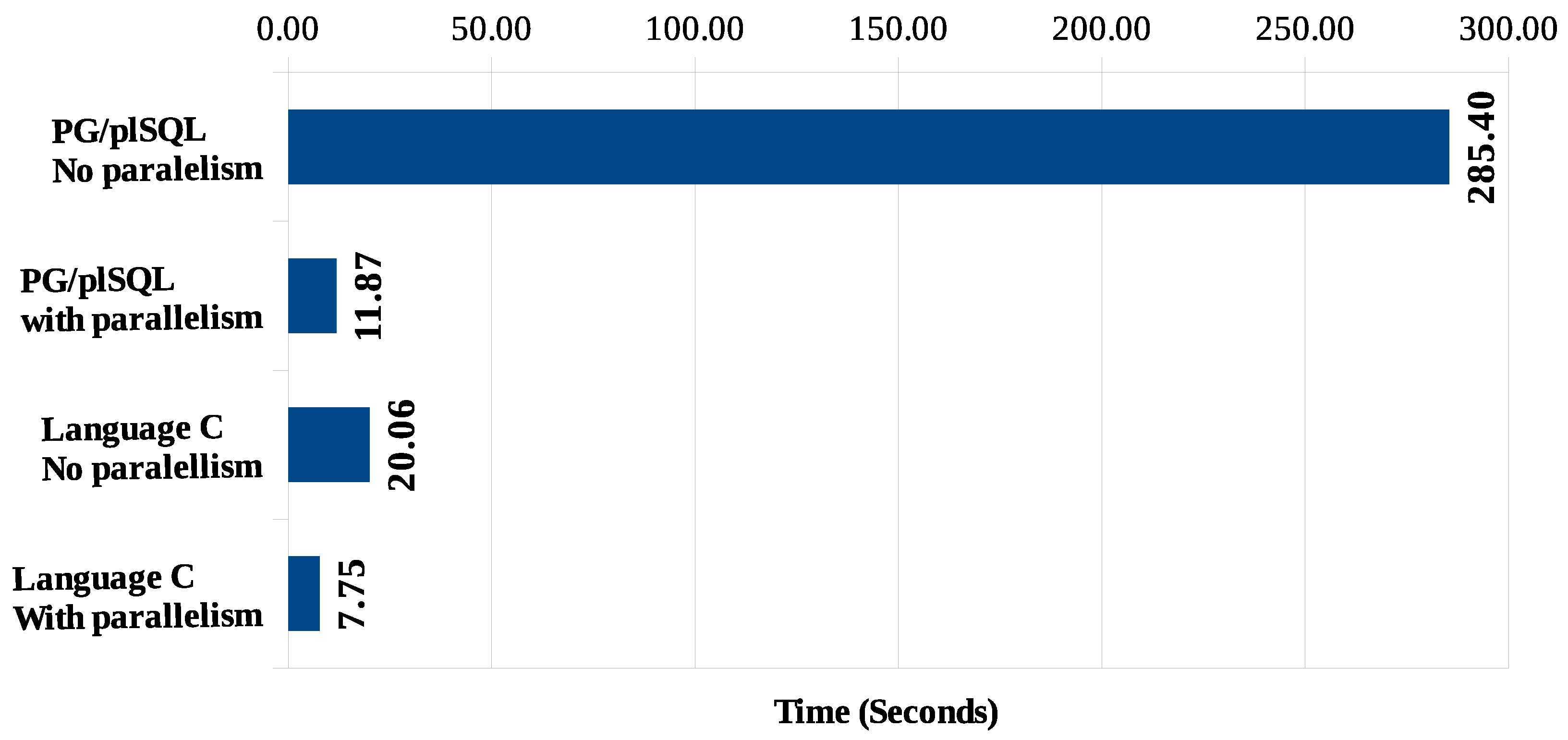
When comparing the lowest possible processing times for each scenario (including the set of algorithms for the identification of pairs of points in proximity, grouping of these pairs and identification of risk indicators), we obtain the graph shown in Figure 19. Scenarios 1 and 3, corresponding to processing without parallelism in PG/pgSQL and in C, respectively, have a final result with higher response times. Scenarios 2 and 4 showed better response times, which became possible due to the utilization of parallel processing for the identification of proximity among coordinate pairs.

In all scenarios, the processing of Algorithms 2 and 3 (detection of groups and computation of risk indicators) is performed with PL/pgSQL language modules due to the good response time obtained with this programming language, which allows the minimum total time to stay at 7.75 s (Scenario 4). Future implementation with all algorithms in C language would further reduce the shortest execution time of the whole process.

This paper does not address the integration of routines in C language being activated by calls from PL/pgSQL functions, a feature supported by PostgreSQL 9. It is estimated, however, that the execution times of the routines in this situation are very close to those measured in our presented scenarios.

4.6. On the Feasibility of Using Distributed Processing

As parallel processing with multiple threads performed better compared to single thread, both in PL/pgSQL and in C language, it is therefore natural to think of an experiment in a distributed processing environment in a big data-oriented architecture. In this context, one of the most frequently-used platform is Hadoop. However, some features of this type of processing should be considered:

(a)

Big data assumes a massive amount of data to be processed. It seems that this is not the case described in this paper. Although high performant processing is implied by application requirements, the amount of data processed at a time (for instance, the 10,000 points proposed here) is not an impressive data volume. As a result, without any special configuration, loading these data into a multiple node environment as expected in a big data environment, this volume of data tends to be loaded on a single node, thus eliminating the possibility of distributed processing. As discussed by Davenport [24], the term big data is basically defined in terms of volume, variety and velocity, characteristics that guide the implementation of big data platforms. The first characteristic (volume) is already compromised in our use case.

(b)

To be treated in a distributed processing environment, the whole process takes a few seconds (in some cases, even minutes) to be ready for processing. This necessary initial time can make it unfeasible to meet the initial requirement described in our problem, which assumes a 1-min time window to perform data samples’ processing, in our case with the 10,000 simulated coordinate points for our validation.

It seems that the applicability of the presented algorithms for distributed processing with the big data Hadoop platform, though it can be useful if anklet monitoring is expanded to larger populations, is still an issue to be investigated, since although the offered processing capacity is relatively higher, the amount of data to be processed is low, but requires important preparation effort, which makes big data for now unsuitable as an alternative solution to the problem.

5. Conclusions

The process of monitoring convicts by means of electronic anklets can be improved by producing additional data to support risk analysis for decision making. In this paper, the challenge of identifying a gathering of groups of monitored convicts, the time of permanence of these groups and the number of their members was proposed with the addition of a limited processing time restriction. The use of serial algorithms was shown to be a problem due to their exceeding processing response time. It was observed that the longest processing time concerned the calculation of pairs of device coordinates regarding their proximity.

The proposed solution to increase performance is the division of the total geographical area containing all coordinate points into smaller areas (quadrants) so that each area can be processed independently, thus allowing parallel processing when identifying points of proximity. Dividing the total area into smaller areas involved dealing with the situation where the points in proximity were in adjacent subareas, which was solved by expanding each area by the GPS precision factor (10 m) in all directions and the elimination of duplicates in the grouping of points in proximity.

The adoption of routines using PL/pgSQL for implementing the algorithms alone would not meet the required time window. However, when using a low-level language, such as C, to implement the same algorithms, the overall response time experiences a substantial reduction.

This response time reduction, however, does not justify giving up parallelism in the proposed processing, since even the routine time in C language without using parallelism (which corresponds to approximately 1/4 of the defined window limit) could compromise the performance requirement. For instance, a linear increase in the number of points to be processed increases exponentially the number of comparisons to be performed to calculate the distance, which directly impacts response time. In this case, even adopting the C language to implement the routines relating to the proposed algorithms, it is appropriate to use a parallel processing solution.

Computing with Graphics Processing Units (GPU) is appropriate in cases of short and parallel routines, as is the case of the detection of nearby points by calculating and comparing distances. Although restricted to specific hardware, but abundantly available on the market, this alternative should be considered in the case of the need for even greater reduction in the response time for the algorithms addressed in this paper. While GPU-accelerated computing should be considered in future works due to the intense and parallel processing characteristics or the pair detection algorithm, other big data platforms, such as Hadoop, can be further studied and tested, in order to address a simplified manner to reach the process performance requirements.

Unlike other algorithms, the solution proposed in this paper includes the monitoring of formed groups over time, periodically updating the data of each group, thus supporting the analysis based on group duration (the time interval in which the group remains assembled) and on the average number of elements of the group during its existence. Moreover, when considering inactive groups (those that have been identified in the past and are now ended), the frequency and time at which certain groups usually meet can also be informed.

We emphasize that this paper is dedicated to issues related to proximity calculations and their performance, although we recognize that there are several other issues equally important to be treated, such as the date-related fusion aspects addressed by Khalegui [9] who classified the related questions as imperfection, correlation, inconsistency and disparateness issues. Thus, the data used in our simulations could be modified and completed to represent situations prone to these problems. Then, for our algorithms to be tolerant to these data quality problems, they must include filters with respect to data characteristics, as for instance invalid dates, eventually missing points, repeated or delayed point collections, etc.

Other issues related to the mobility of groups will be addressed in future work due to the complexity of their identification and treatment. Such problems occur, for example, when there is a tracked device in a meeting and this device fails to submit the coordinates, thus causing the wearer to be considered outside the group in the corresponding periodic processing. Indeed, groups identified and tracked, being stationary or on the move, are handled the same way in the proposed algorithms, although each of these situations may pose different risks.

The integration of the data produced in this work with other complementary databases, such as those registering crimes occurring at the same time and location of the meetings detected, and the registry of individual dangerousness are important to increase and improve the information made available to the investigation teams. Such integration should be addressed as future work.