Globally Consistent Indoor Mapping via a Decoupling Rotation and Translation Algorithm Applied to RGB-D Camera Output

Abstract

This paper presents a novel RGB-D 3D reconstruction algorithm for the indoor environment. The method can produce globally-consistent 3D maps for potential GIS applications. As the consumer RGB-D camera provides a noisy depth image, the proposed algorithm decouples the rotation and translation for a more robust camera pose estimation, which makes full use of the information, but also prevents inaccuracies caused by noisy depth measurements. The uncertainty in the image depth is not only related to the camera device, but also the environment; hence, a novel uncertainty model for depth measurements was developed using Gaussian mixture applied to multi-windows. The plane features in the indoor environment contain valuable information about the global structure, which can guide the convergence of camera pose solutions, and plane and feature point constraints are incorporated in the proposed optimization framework. The proposed method was validated using publicly-available RGB-D benchmarks and obtained good quality trajectory and 3D models, which are difficult for traditional 3D reconstruction algorithms.

1. Introduction

Complete 3D models of the indoor environment are an important part of modern digital city systems [1,2]. However, the collection of 3D model data for the indoor environment is not as easily achieved for those outside, especially for globally-consistent 3D models [3,4]. Indoor 3D model helps GIS (Geographical Information System) to represent, interpret and manage communities and cities [5]. Many kinds of sensors are employed to measure cities in 3D space, for example LiDAR on a movable car can capture a 3D model of streets. Cameras and LiDARs on a UAV (Unmanned Aerial Vehicle) can scan large portions of the Earth’s surface. This information is already used in many fields such as environment monitoring and urban planning. The need for indoor 3D models increases with the need more inclusive and smarter cities. Indoor 3D models also play an important role in fire and rescue [6], building evaluation [7], and so on.

Indoor 3D models are increasingly in demand in many fields [8]; however, most of the mapping techniques are limited to the outside environment. Cameras used outside have a larger field of view, and GPS (Global Position System) can usually provide an acceptable global position, thus making an outdoor 3D model relatively straightforward and high quality [9]. Moreover, the larger field of view makes the task more productive. To get an indoor 3D model, we have to scan a variety of poses and positions, because of both the narrow field of view and the complex layout of the indoor space. Information from one scan in the outdoor environment covers a significantly larger area than that of the inside. For the outside, the platform is usually equipped with GPS and IMU, which help to locate the camera poses. Furthermore, the camera can capture more features in each scan, which means that it is rare to encounter a case where a camera only captures a white wall for which few interest points can be extracted. In our case, we propose an algorithm that is robust enough for a flexible hand-held RGB-D camera scanning the indoor environment.

Indoor localization is a big topic in GIS applications. It requires a 3D indoor map as the basic information. With the help of a mobile phone or other smart device, it can provide localization and navigation services for the public in complex indoor scenarios, for example hypermarkets and office buildings. These services can only be provided if the indoor map has already been created. In firefighting scenarios, if the emergency team members are supported by the 3D GIS system, they can get instant information of how the flames are spreading in the environment and can take the most efficient measures to stop them. More importantly, the firefighter will know if he/she can retreat safely, guided by a known indoor map and other instant information that can be integrated into one GIS system. At the same time, this information can be delivered to the commanding office, and the commanding officer can make better decisions. For an image without the 3D indoor map, these applications will be restricted.

The RGB-D camera provides an affordable and effective solution to obtain indoor 3D models [10,11,12]. One of the famous RGB-D cameras is the Kinect, integrating an RGB camera and a depth camera. There are several kinds of RGB-D sensors, such as Microsoft V1 and V2, Intel RealSense and Xtion. For simplicity, in the following we refer to the RGB-D camera as Kinect V1, as the hardware may differ a little, but it is independent of the algorithm. RGB-D cameras integrate an RGB camera and a depth camera, which is composed of an IR (Infrared) projector and an IR receiver. RGB images of 640 × 480 pixels and depth images of 320 × 240 pixels are produced when scanning. The first applications of these cameras were to track a hand pose in front of it, thus achieving human-machine intervention. Later, the camera has proven useful in various fields, including SLAM (Simultaneous Localization And Mapping), navigation, and obstacle avoidance for robots [13]. Recently, the camera has shown potential for use in 3D reconstruction and performs well if the noise is carefully handled. Compared with costly 3D lasers, which can be used in extremely high-quality 3D reconstruction tasks, RGB-D cameras are more flexible and suitable for general purpose 3D reconstruction tasks.

As a consumer RGB-D camera, the accuracy of the depth camera is not as good as laser scanners and also not stable [14]. Firstly, the resolution of the depth image is half the size of the RGB image. For registration, the camera has to upsample the depth image to internally match the RGB image. Moreover, the accuracy of the depth image does not only depend on the hardware, but also the structure of the environment. The points at the edge of an object are noisier than those on a plane. On some materials, the reflection will affect the measurement of depth. All the above phenomena increase the uncertainty of the camera, which is carefully dealt with in our algorithm.

In point-based 3D reconstruction, the data association step associates the points in one frame to the points detected in other frames. Correct data association is a basic precondition for converging to the right solution. However, if there are many errors in data association, the optimization usually does not converge well. Incorrect data associations and high uncertainty of point features are the two main reasons that traditional Bundle Adjustment (BA) does not perform well for this task.

In the indoor environment, we encounter white walls and monotone-colored tables with few visual features. They are usually ambiguous, since the color patterns are monotonous or repeat. Compared with point features, there are no effective descriptors for planes. Planes are not handled well enough by traditional methods. Though the planes lack color information, they provide much information about the structure of the environment. In our study, we utilized the planes to constrain points on them and hence propagated the information to poses.

Computational burden is another problem for visual-based 3D reconstruction. As every frame observes hundreds of visual features and the frames increase linearly with the size of the environment or the scanning time, the algorithm cannot handle all the variables in one optimization problem. One solution to this issue is to use a keyframe scheme. In this case, the problem will be limited to poses and features only on chosen keyframes, meaning the algorithm can be implemented on movable platforms.

In our study, the algorithm should estimate the poses of cameras and simultaneously estimate the position of the features in 3D space. Though 3D reconstruction and structure from motion have gained much progress in recent years [15,16], it is still difficult to obtain a globally-consistent 3D indoor model using only RGB-D cameras. We propose a novel 3D reconstruction method that decouples rotation and translation to obtain more robust pose estimation. Different from traditional BA, which directly utilizes 3D measurements from the depth image, our algorithm uses an elegant method to incorporate noisy depth measurements. In absolute rotation estimation, the algorithm only utilizes the feature points from RGB images and produces an accurate rotation estimation and a rotation without scale. Next, it calculates a one-to-one correspondence for all the pixels in the matching frames and estimate an absolute translation using all the depth information. In every keyframe, it applies a plane extraction method to extract the plane areas from the depth image. The planes and feature points are then associated using a simple thresholding method. The poses, feature points and planes are then incorporated into a unified framework.

As shown in Figure 1, the only inputs to the algorithm are RGB images and depth images from an RGB-D camera. To avoid inaccuracies introduced by the depth image and to make full use of the relatively accurate color image, we estimate an accurate rotation from the color images only. The accuracy from the color images is more robust and independent of the environment. An absolute translation is then calculated using the measurements from depth images. Utilizing the constraints from planes is intuitive, as the measurements from images rely on the rays, which contain robust information in one direction. In indoor environments, the plane structure is a common feature and delivers valuable information about the structure of the space. In a multiple camera system, we should always consider the synchronization problem. As synchronization problems occurs with random noise, it is hard to find a simple way to compensate. The synchronization problem affects the accuracy of depth measurement, which means that the depth measurement considered may not be the one corresponding to the color image, it may be the depth measurement from nearby pixels. However, this problem is alleviated by the use of planes used in our proposed method.

In summary, our study contributes in three ways:

• A 3D reconstruction algorithm is proposed, which decouples the estimation of the rotation and absolute translation of the camera poses. Note that we do not decouple the rotation and arbitrary translation completely, as we use these as the initial values for further processing.
• We incorporate the constraints between planes and points in the estimation problem, which contributes to the robustness of the algorithm.
• The qualitative and quantitative comparisons on various datasets show that the proposed 3D reconstruction algorithm is accurate, robust and effective.

The method is organized as follows: Some related work is discussed in Section 2. The proposed method is described in Section 3. Specifically, this comprises the visual feature detection in Section 3.1, uncertainty of depth measurements in Section 3.2, rotation solving in Section 3.3, absolute translation recovery in Section 3.4, plane constraints in Section 3.5 and joint optimization in Section 3.6. Section 4 presents the experiments and results. Section 5 concludes the paper and gives some future work about this method.

2. Related Work

In different fields, for example, computer graphics, photography, computer vision, augmented reality, and robotics, 3D reconstruction using RGB-D cameras has been studied for various kinds of applications [11,17,18]. In the following, we introduce the work most related to our study. We also cover some work related to techniques in this study, such as feature extraction.

In [19], a coarse registration of the RGB-D sequence was done using 3D points based on SIFT and depth measurements, where they carefully weighted the theoretical random error based on the novel disparity model. The work in [20] proposed an epipolar search method for point correspondence and defined the 3D point weights according to a theoretical random error of depth measurements. The work in [21] introduced a novel hybrid “continuous stop-and-go” mobile mapping system, which integrates an MEMS IMU and two Kinect sensors. As the IMU can produce relative pose transformations for short sequences, and the system can deal with textureless walls and areas with many occlusions. The work in [22] placed all the rotation parameters into a common coordinate system by exploiting a property of quaternions, then a global refinement procedure was applied. They evaluated their algorithm on a TLS (Terrestrial Laser Scanner) dataset and presented its effectiveness. Online 3D SLAM [23] introduced a fast pose-graph relaxation technique for large planar surface patches, for which a loop-closing was needed due to the lack of surfaces in certain directions, resulting in translation uncertainty. A coarse to fine framework was proposed in [24], in which the most interesting contribution was that they posed the task of finding a global alignment as picking the best candidates from a set of putative pairwise registrations. The work in [25] extended the 2D pose estimation methods to 3D poses with six degrees of freedom, resulting in non-linearities. A classical method using Taylor expansion and Cholesky decomposition was used to deal with the massive amount of 3D data. In [26] all the local frames of data and the relative spatial relationships between them were defined as random variables and formulated as a procedure based on the maximum likelihood criterion.

The work in [27] proposed rotation and translation decoupling methods. They first computed the relative pairwise rotations, outliers of which were detected using sequential Bayesian inference. The consistency of the rotation matrix was thus improved and translated from the relative to the global coordinate system. Next, they fixed these rotations and formulated the estimation of relative translations with convex optimization. This paper [28] introduced a global, robust rotation estimation method based on combined weighted averaging, which can detect outliers in an effective and robust way. These works aimed to reconstruct a 3D model using pure images, and in most cases the quality (or resolution) of these images was very high. It was more challenging in our case, as the resolution problem and motion blurs were very common.

Real-time SLAM: In the field of robotics, most work is focused on a real-time 3D reconstruction, as the robot needs a map for localization and path planning [12,15,29]. As the robot platform usually has a less powerful computer, off-line computation-intensive algorithms are not suitable. The work in [30] provides a unified framework for monocular, stereo and RGB-D cameras. The algorithm can switch easily between different sensors. It translates the depth image to a stereo disparity image using a user-defined baseline. One advantage of this transformation is that it put both the feature measure and depth measurements into pixel units. However, it also uses measurements from depth images directly, and the uncertainty model of the depth measurements was not well studied. The work in [31] combined measurements from the depth and RGB images, and is suitable for large environments. The Kinect fusion reduced the noise in the depth image by ray casting a synthetic depth image from a previous model [11]. The synthetic depth image, from n observations, is smoother and more accurate, and is registered with the current depth image to get a relative pose estimation. Kinect fusion can give a consistent model when scanning a object that is not large.

Global registration with loop closure: Loop closure is a technique that utilizes the fact that the camera will revisit (rescan) the same place. If the algorithm detects that an image has been scanned before, new constraints are inserted. In monocular reconstruction, the scale fits the first two frames, so it is likely that the scale will drift over a long scanning sequence. The scale error accumulates as time goes by. Loop closure can fix the scale drift and ease the accumulated error. RGB-D reconstruction can also use this technique to obtain a globally-consistent 3D model. Retrieving similar images from the database is an essential procedure for this task. The work in [32] proposed a bag of visual words to retrieve similar images. The work in [33] used randomized fern encodings to do the retrieval. Recently, deep learning was also utilized for this task [34]. In our study, retrieved images are not our focus, so we employed a classical bag of visual words method to get loop closure. As shown in

Table 1. Comparisons of related works in terms of feature types, running time, depth uncertainties, decoupling rotation and translation.

Algorithm/Evaluation	Whelan [33]	Endres [10]	Whelan [29]	Xiao [35]	Concha [31]	Halber [36]	Santos [19]	Vestena [37]
Features	Patches	Points	Points	Points	Points	Points Planes	Points Regions	Points
Real time	Yes	Yes	Yes	No	Yes	No	No	No
Uncertainty model	No	No	No	No	No	No	Yes	Yes
Decoupling	No	No	No	No	No	No	Yes	Yes

, we compare some state-of-the-art methods on feature types, running time, depth uncertainties, decoupling rotation and translation.

Point feature and plane extraction: There have been many visual feature extraction algorithms proposed in recent years, all of which aim to achieve scale-invariant, illumination-invariant, and rotation-invariant properties. Only with these properties can the matched visual features be extracted from different frames. To develop a real-time application algorithm, our method applied Oriented fast and Rotated Brief (ORB) to extract visual features, which is more computationally efficient. Plane extraction is also a basic part of our method. To detect the spatial relationship of points [38], proposed to search nearby points in the image space instead of searching in 3D space, which usually requires building a KD-tree for each point cloud for a faster search. Though judging the relationship in 2D space is not justifiable, for the plane extraction the points on the same plane should lie on the nearby pixels. The work also proposed a fast plane extraction method, and we used the framework from there and improved on it. We clustered the points in a two-step fashion: clustering on normals and clustering on locations.

3. Methods

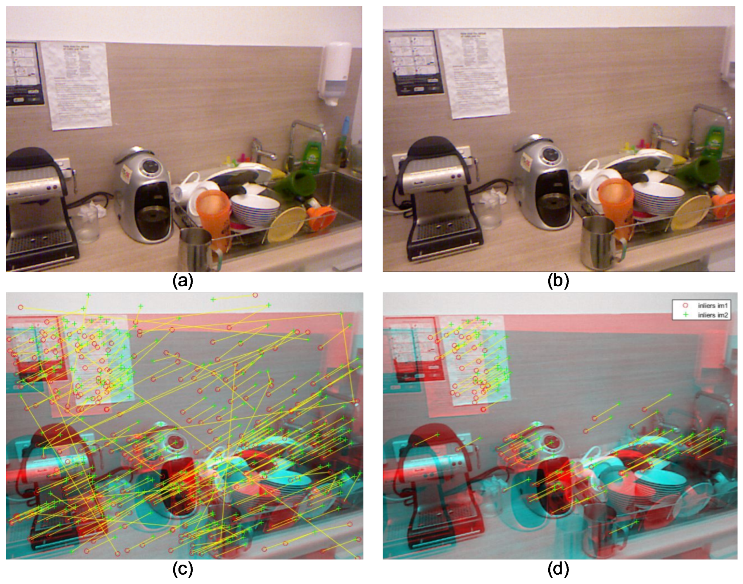
3.1. Visual Feature Detection

In computer vision, various feature extraction methods have been proposed, for example Scale-Invariant Feature Transform (SIFT) [39] and Speeded Up Robust Features (SURF) [40]. The work in [41] proposed Oriented fast and Rotated Brief (ORB) by combining fast corner detection and BRIEF feature descriptors and achieved state-of-the-art results in terms of efficiency and accuracy. ORB is especially suitable for movable platforms where computation resources are extremely limited. Sensitivity to noise and rotation variance of the BRIEF descriptor was also improved. Figure 2 shows two RGB images on the top row, which are two keyframes used by our algorithm. The bottom left image presents the result of the ORB feature extraction and matching using Hamming distance. The bottom right image shows the refined matches using after RANdom SAmple Consensus (RANSAC).

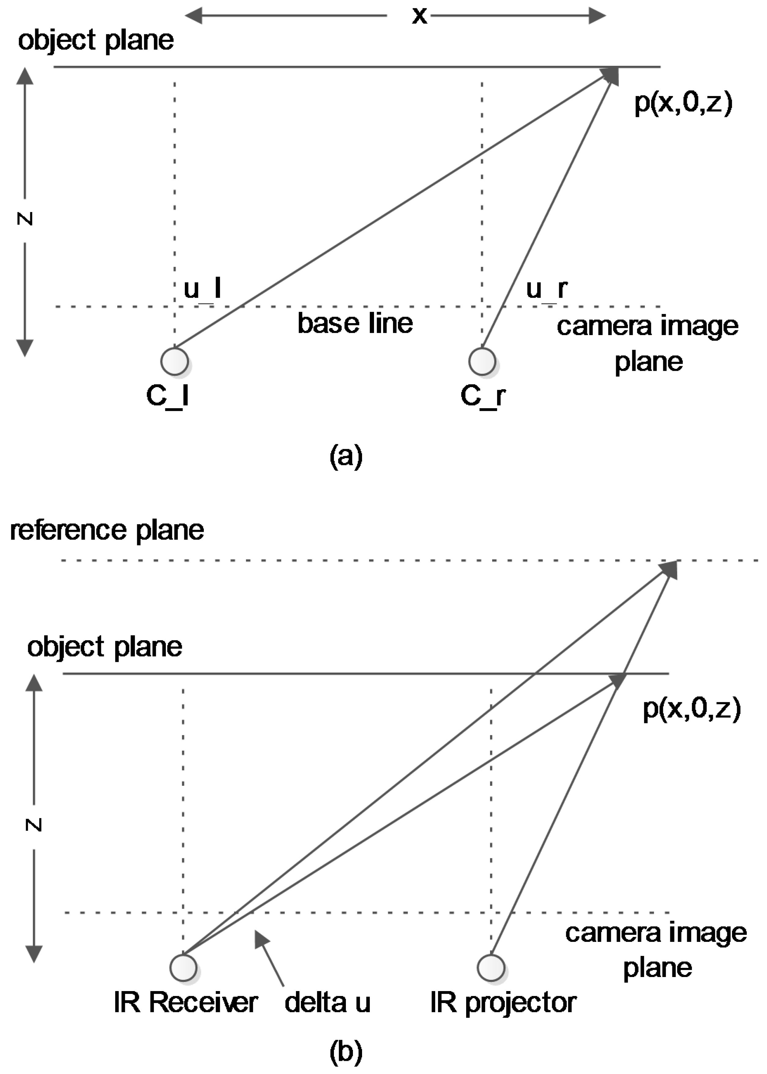
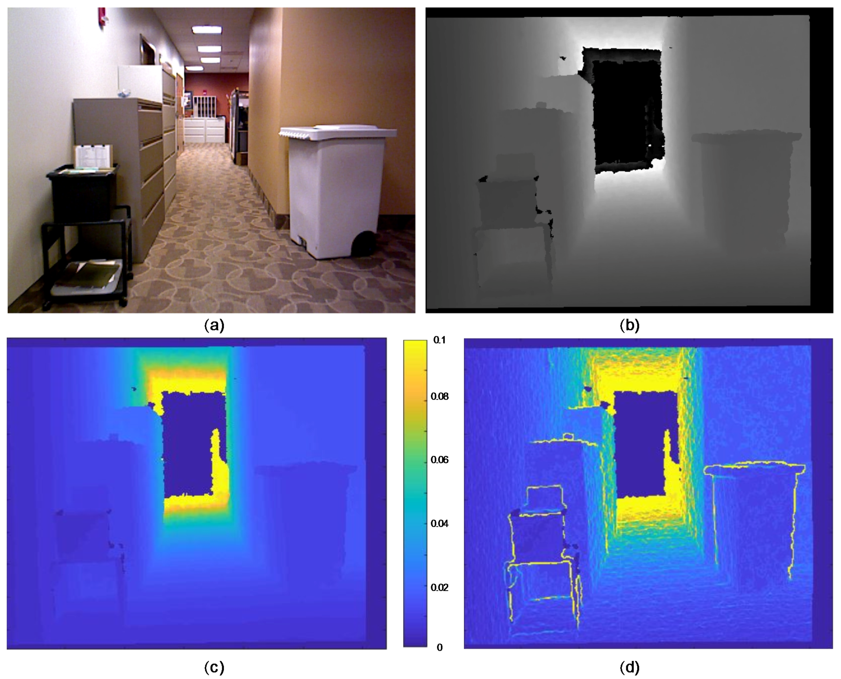
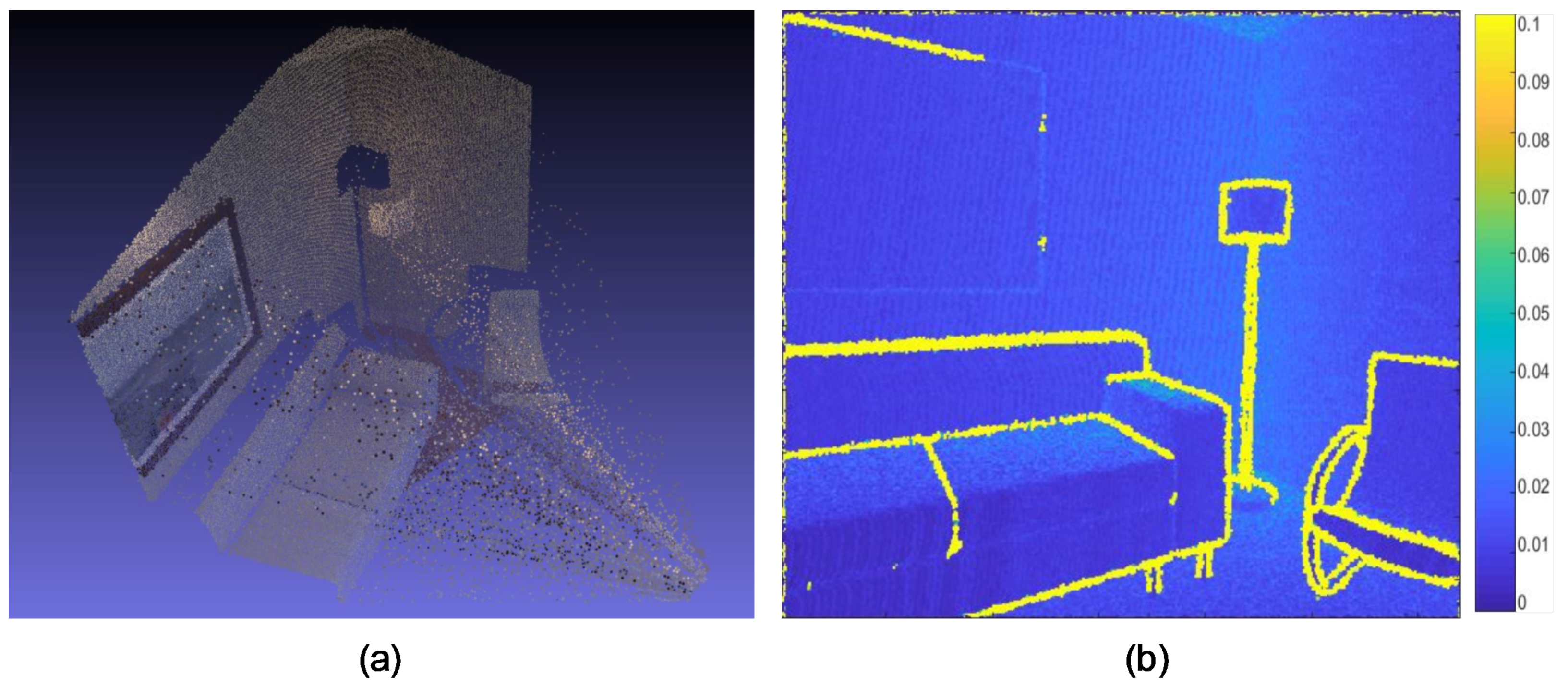
3.2. Uncertainty of Depth Measurements

In this section, we describe the uncertainty model for RGB-D cameras. For simplicity, we use the Kinect v1 camera as an example. The work in [14] gave an uncertainty model for the RGB-D camera based on the observation that the farther the object, the noisier the measurement will be. Like the standard stereo camera, the RGB-D camera also gives a disparity measurement and transforms it to depth values. However, the value has a slightly different meaning than the standard disparity values. In Figure 3, the top panel shows the classic stereo camera model. We supposed that the images have been rectified. In the left camera frame, the object point is $p(x,0,z)$, while in the right camera frame, it is $p(x-b,0,z)$. According to the properties of similar triangles, we have:

$$\begin{array}{cc}\hfill \frac{f}{x_l}& =\frac{z}{x}\hfill \\ \hfill \frac{f}{x_r}& =\frac{z}{x-b}\hfill \end{array}$$

(1)

where f is the focal length, b is the baseline, $x_l$ is the horizontal pixel values in the left camera frame and $x_r$ is the horizontal pixel values in the right camera frame. The disparity value is given as:

$$v_{disparity}=x_l-x_r=\frac{fb}{z}$$

(2)

However, the disparity value of the RGB-D camera is different from that of the stereo camera. As shown in the bottom figure in Figure 3, the left camera is an IR receiver camera, and the right one is an IR projector camera. $Z_0$ denotes a virtual reference plane, which is the maximum distance that a Kinect can measure. The object is also denoted by $p(x,0,z)$. The following equation defines that the disparity value as the subtraction of the object disparity value from the corresponding disparity value:

$$d=d_k-d_0=fb(1/z_k-1/Z_0)$$

(3)

where $d_k$ is the disparity value for object p and $d_0$ is the disparity value for corresponding points on the reference plane. We can obtain the relationship between $z_k$ and d:

$$z_k=\frac{Z_0}{1+\frac{1}{fb}d}$$

(4)

For simplification, Khoshelham et al. [14] derived the variance of z as:

$${\sigma }_z=\frac{1}{fb}{\sigma }_{d^{\prime }}{\mu }_z^2$$

(5)

where $d^{\prime }$ is the normalized version of d defined in [14], and ${\sigma }_{d^{\prime }}$ is a parameter of the RGB-D camera device. They calibrated the ${\sigma }_{d^{\prime }}$ using repeated experiments. In the following, we will use the value ${\sigma }_{d^{\prime }}$ reported in the study.

In our study, we observed that the uncertainty of depth measurement is not only related to the camera device itself, but also to the structure of the environment. For example, when the environment is flat the measurements are more accurate and without much noise. However, for a cluttered environment with many different features in the background and foreground, the depth image is more noisy.

Based on the variance values from Equation (5) and the Gaussian mixture, we improve the uncertainty model from the single depth pixel to multi-window cases, considering the adjacent structures of the environment. In our experiments, we employed two window sizes, a smaller one using even areas and a larger one using clustered areas. Two weight matrices were defined for the two windows.

$$\begin{array}{c}\hfill W_{3\times 3}=\frac{1}{16}\left[\begin{array}{ccc}1& 2& 1\\ 2& 4& 2\\ 1& 2& 1\end{array}\right]W_{5\times 5}=\frac{1}{52}\left[\begin{array}{ccccc}1& 1& 2& 1& 1\\ 1& 2& 4& 2& 1\\ 2& 4& 8& 4& 2\\ 1& 2& 4& 2& 1\\ 1& 1& 2& 1& 1\end{array}\right]\end{array}$$

(6)

From Equation (5), we know that the depth measurement z from pixel $(i,j)$ follows a Gaussian distribution, i.e., $z_{i,j}\sim N({\mu }_{z_{i,j}},{\sigma }_z)$, where ${\mu }_{z_{i,j}}$ is the mean value and ${\sigma }_z$ is the variance. We took the measured depth value as the mean value and calculate the variance using Equation (5). However, this kind of uncertainty model only includes the system error from sensors and ignores the effect of the layout of the environment, as described in Figure 4.

In our uncertainty model, we included the uncertainty of adjacent pixels using the weight matrix defined in Equation (6). For the pixel at $(i,j)$, we can derive the uncertainty of the depth measurement using a Gaussian mixture. The mean value is the weighed mean value from several pixels within the window.

$${\overline{u}}_z=\sum _{k_1=-W_{s^{\prime }}}^{W_{s^{\prime }}}\sum _{k_2=-W_{s^{\prime }}}^{W_{s^{\prime }}}{W}_{i+k_1,j+k_2}{u}_{z_{i+k_1,j+k_2}}$$

(7)

where $W_s$ is the size of the weight window and $W_{s^{\prime }}=\frac{W_s-1}{2}$ is half the window size. The variance is defined as:

$$\overline{{\sigma }_z^2}=\sum _{k_1=-W_{s^{\prime }}}^{W_{s^{\prime }}}\sum _{k_2=-W_{s^{\prime }}}^{W_{s^{\prime }}}{W}_{i+k_1,j+k_2}({\sigma }_{z_{i+k_1,j+k_2}}^2+{\mu }_{z_{i+k_1,j+k_2}}^2)-{\overline{u}}_z^2$$

(8)

In this definition, the variance includes information from adjacent depth pixels. If the depth values vary greatly in the window (around the edge of the object), the uncertainty will also increase to describe this accordingly.

Figure 4a,b shows a pair of an RGB color image and a depth image. There are some objects in the scene, and we can see the noise around the edges of the objects. Figure 4c presents the uncertainty model using independent pixel methods; the variance increased in line with the depth values, which are the system errors from the device. As expected, the noise around the edges of objects is not captured by the uncertainty model. Figure 4d shows the results from our method, which inherits the system noisy from the device and also incorporates the noise around the edges. A more intuitive noise example is given in Section 4, where the noises are visualized in 3D space.

3.3. Rotation Solving

For RGB-D cameras, the depth image suffers from noise. Traditional RGB-D reconstruction methods use the depth values directly, which influences the performance of these method. In our algorithm, we only use RGB images to estimate the rotation matrix of the camera pose.

For simplicity, we take two RGB images $Im{g}_l,Im{g}_r$ as an example; the subscripts $l,r$ indicate the left and right image. Firstly, visual features are extracted and matched using the method described in Section 3.1. Secondly, the eight-point algorithm and RANSAC are applied to get a pose guess for the two frames [42]. Thirdly, the pose from the previous step is used as the initial values and optimized in the current step. The details of this optimization problem are described below.

The variables to be optimized are feature points in 3D space $p\in {\mathcal{R}}^3$, the camera pose $\mathcal{T}\in SE\left(3\right)$ and the pixel values of feature points on the left and right RGB image ${\widehat{I}}_l,{\widehat{I}}_r\in {\mathcal{R}}^2$. The energy function is defined as:

$$E_R=\sum _{i=1}^m\left|\right|K{p}_i-{\widehat{I}}_l{\left|\right|}_{{\Sigma }_{uv}}^2+\sum _{i=1}^m\left|\right|K\mathcal{T}{p}_i-{\widehat{I}}_r{\left|\right|}_{{\Sigma }_{uv}}^2$$

(9)

where m is the number of matched feature points between the two frames, K is the intrinsic matrix of the camera, ${\Sigma }_{uv}$ is the covariance matrix of the $uv$ measurements, which is set to an identity matrix, and the subscript $uv$ indicates image columns and rows. We define two functions to denote the two terms in the above energy function and leave the subscript i for simplicity.

$$\begin{array}{ccc}\hfill f_1\left(p\right)& =& Kp-{\widehat{I}}_l\hfill \\ \hfill f_2(R,T,p)& =& K\mathcal{R}p-{\widehat{I}}_r=K(Rp+T)-{\widehat{I}}_r\hfill \end{array}$$

(10)

where pose $\mathcal{T}$ can be rewritten as a combination matrix of rotation $R\in SO\left(3\right)$ and translation $T\in {\mathcal{R}}^3$: $\mathcal{T}=[R,T]$.

For the first function, applying a first order Taylor series expansion gives:

$$\begin{array}{cc}\hfill f_1^r(p+\Delta p)& \approx f_1^r\left(p\right)+\frac{\partial f(p+\Delta p)}{\partial p}\Delta p\hfill \end{array}$$

(11)

where $\Delta p\to \mathbf{0}$. The Jacobian matrix can be expressed as:

$$\frac{\partial f_1(p+\Delta p)}{\partial p}=K𝟙$$

(12)

where $𝟙$ denotes the identity matrix.

In the second function, we define the first order Taylor series in a similar way. As $p,T\in {\mathcal{R}}^3$, the corresponding Jacobian matrix can be defined as:

$$\begin{array}{cc}\hfill \frac{\partial f_2(p+\Delta p)}{\partial p}& =K(R𝟙)\hfill \\ \hfill \frac{\partial f_2(T+\Delta T)}{\partial T}& =K(T𝟙)\hfill \end{array}$$

(13)

The rotation R is a little complicated, and we introduce some basic concepts before defining the Jacobian matrix. $R\in SO\left(3\right)$ is a special orthogonal group, which is a Lie group. A Lie group is a topological group that is also a smooth manifold and has attractive properties. Every Lie group has an associated Lie algebra, which is the tangent space around the identity element of the group. In our case, the associated Lie algebra is $SE\left(3\right)$. We cannot add a small value to R in the way that we do in Euclidean space. A special plus operator should be defined to achieve this. Suppose that $ϵ\in {\mathcal{R}}^3$ is a small increment. A skew symmetric operator is defined as:

$${ϵ}^{\wedge }={\left[\begin{array}{c}{ϵ}_1\\ {ϵ}_2\\ {ϵ}_3\end{array}\right]}^{\wedge }=\left[\begin{array}{ccc}0& -{ϵ}_3& {ϵ}_2\\ {ϵ}_3& 0& -{ϵ}_1\\ -{ϵ}_2& {ϵ}_1& 0\end{array}\right]\in se\left(3\right)$$

(14)

and a plus operator:

$$R\oplus ϵ=exp\left({ϵ}^{\wedge }\right)R$$

(15)

Applying the small increment to function $f_2$:

$$\begin{array}{cc}\hfill f_2(R\oplus ϵ)& =K\left(exp\left({ϵ}^{\wedge }\right)R\right)p+KT-{\widehat{I}}_r\hfill \end{array}$$

(16)

When deriving a partial derivative, the variables T and p are regarded as known variables, so we can ignore these terms for simplicity. For a very small increment $ϵ$, we apply the first order Taylor series expansion.

$$\begin{array}{cc}\hfill K\left(exp\left({ϵ}^{\wedge }\right)R\right)p& \approx K(exp\left(\mathbf{0}\right)+{ϵ}^{\wedge })R)p\hfill \\ & \approx K(𝟙+{ϵ}^{\wedge })Rp\hfill \\ & \approx KRp+K{ϵ}^{\wedge }Rp\hfill \\ & \approx KRp-K{\left(Rp\right)}^{\wedge }ϵ\hfill \end{array}$$

(17)

From the equation above, we determine that the partial derivative over R is:

$$\frac{\partial f_2(R+\Delta R)}{\partial R}=-K{\left(Rp\right)}^{\wedge }$$

(18)

The optimization problem can be solved using the LM (Levenberg Marquardt) algorithm. The full Jacobian matrix can be computed using Equation (19). The row of the full Jacobian matrix is a combination of all the object functions, and its columns comprise a mixture of all variables. An example Jacobian matrix is:

$$J_r=\left[\begin{array}{cccc}\mathbf{0}& \mathbf{0}& \dots & \frac{\partial f_1\left(p_i\right)}{\partial p_i}\\ \frac{\partial f_2(R,T,p_i)}{\partial R}& \frac{\partial f_2(R,T,p_i)}{\partial T}& \dots & \frac{\partial f_2(R,T,p_i)}{\partial p_i}\\ \dots & \dots & \dots & \dots \\ \mathbf{0}& \mathbf{0}& \dots & \frac{\partial f_1\left(p_i\right)}{\partial p_i}\\ \frac{\partial f_2(R,T,p_i)}{\partial R}& \frac{\partial f_2(R,T,p_i)}{\partial T}& \dots & \frac{\partial f_2(R,T,p_i)}{\partial p_i}\\ \dots & \dots & \dots & \dots \end{array}\right]$$

(19)

where $p_i$ is the $ith$ matching points on the two frames. The optimized rotation matrix is considered an accurate solution and remains fixed in the process that follow. The translation T would converge to an arbitrary one if no scale information is provided. An accurate (or absolute) translation will be solved in the next section.

3.4. Absolute Translation Recovery

The absolute translation here means a translation with scale. In the previous section, we solved an accurate rotation matrix and an arbitrary translation using detected ORB visual feature points. In this section, we propose an algorithm to compute an absolute translation using all the information from the depth image. The proposed method is more robust than traditional ones because it does not rely only on the depth measurements on ORB feature points.

3.4.1. Back Projection Associations

The relative pose has been computed in Section 3.3, and the projection relationship between points has been determined. That is, given a pixel with depth value in frame k, we can find an association pixel in frame $k+1$, or there is no association pixel when the projection is beyond the boundary of the image frame.

Firstly, we compute a ratio between the depth values from depth measurement and those from estimations. We scale the depth image by applying the ratio to all depth measurements. Then, we back project the pixels from left image frame $I_j^l$ to 3D space ${\widehat{p}}_j^l$. Point ${\widehat{p}}_j^l$ is then transformed to the correct image frame using:

$$I_j^l=K\mathcal{T}{\widehat{p}}_j^r$$

(20)

where j is the $jth$ pixel from the image; in the typical case, $j\in \left\{integer\right|0<j<640\times 480\}$. Unlike the depth image estimation from Section 3.3, $\widehat{p}$ is rescaled by applying a ratio. We transform all the points using Equation (20), and an association pixel will be obtained if the projected pixel lies inside the valid range of the images. Most of the depth images are noiseless except those near the edges and those far away. In traditional methods, using the depth values of visual features suffers from noise, as they could not ensure that the visual feature points are not from edges or those far away. In fact, many visual features are located near edges, as the edges usually have salient pixel value changes. In the proposed algorithm all the pixel points, including visual features and non-visual features, are included when predicting a robust pose estimation.

3.4.2. Solve Translation

In Section 3.3, the rotation part in pose $SE\left(3\right)$ has been estimated and will be fixed here. The translation part will be estimated here using the point associations in the last section. An energy function is defined as:

$$E_T=\sum _{j=1}^{640\times 480}\left|\right|\mathcal{T}{\widehat{p}}_j^r-{\widehat{p}}_j^l{\left|\right|}_{{\Sigma }_{xyz}}^2$$

(21)

where ${\widehat{p}}_l,{\widehat{p}}_r$ are the points from the depth image in the left and right frames and ${\Sigma }_{xyz}$ is the covariance matrix for the points and can be expressed as:

$$P_{xyz}=\left[\begin{array}{ccc}{\sigma }_x^2& {\sigma }_{xy}& {\sigma }_{xz}\\ {\sigma }_{yx}& {\sigma }_y^2& {\sigma }_{yz}\\ {\sigma }_{zx}& {\sigma }_{zy}& {\sigma }_z^2\end{array}\right]$$

(22)

To compute the covariance for $x,y,z$, the pinhole camera model will be used:

$$\begin{array}{cc}\hfill x& =\frac{z}{f_x}(u-c_x)\hfill \\ \hfill y& =\frac{z}{f_y}(u-c_y)\hfill \end{array}$$

(23)

Based on the uncertainty defined in Section 3.2, we can derive the covariance as follows:

$$\begin{array}{cc}\hfill {\sigma }_x^2& =\frac{({\sigma }_z^2{(u-c_x)}^2+{\sigma }_u^2{z}^2)}{f_x^2}\hfill \\ \hfill {\sigma }_y^2& =\frac{{\sigma }_z^2{(v-c_y)}^2+{\sigma }_v^2{z}^2}{f_y^2}\hfill \end{array}$$

(24)

$$\begin{array}{cc}\hfill {\sigma }_{xz}& ={\sigma }_{zx}=\frac{u-c_x}{f_x}{\sigma }_z^2\hfill \\ \hfill {\sigma }_{yz}& ={\sigma }_{zy}=\frac{v-c_y}{f_y}{\sigma }_z^2\hfill \\ \hfill {\sigma }_{xy}& ={\sigma }_{yx}=\frac{(u-c_x)(v-c_y)}{f_x{f}_y}\hfill \end{array}$$

(25)

The energy function (21) incorporates as many depth measurements as possible to estimate the translation variables, which is more robust than using only depth measurements for visual features. In Section 4, we see that our method outperformed other methods.

We define another function $f_3$ to describe the third term in the energy function and leave subscript j for simplicity.

$$f_3\left(T\right)=\mathcal{T}{\widehat{p}}_r-{\widehat{p}}_l=R{\widehat{p}}_r+T-{\widehat{p}}_l$$

(26)

From the above equation, we see that the only variable is the translation $T\in {\mathcal{R}}^3$, as rotation R has been fixed. This is a linear least squares problem, with a constant Jacobian matrix:

$$J^t=\left[\begin{array}{c}{I}_{3\times 3}\\ \dots \\ I_{3\times 3}\\ \dots \end{array}\right]$$

(27)

This means that, although we utilize all the depth measurements in our formulation, we can also obtain the solution as fast as other visual-feature-only methods. Compared with the iterated solution in other methods, our methods gave a more robust solution, as they do not suffer from the local minimum problem. Our methods also were efficient in computation time, as there was no need to compute the Jacobian matrix for a large number of depth measurements. In Section 4, a quantity comparison illustrates the benefits of the proposed methods.

3.5. Plane Constraints

In the indoor environment, a plane is a common and important structure. When estimating the pose of cameras, we also predict the position of visual feature points. In the above sections, the constraints between points and image measurements have been incorporated. However, there are also constraints between points themselves, for example some points lie on the same plane, the same line structure or the surface of a small object like a cup. In this paper, we explore the potential use of plane constraints on points to improve the robustness of the algorithm. We follow the method in [30] to choose a keyframe when the visual points detected are sufficiently different. Then, a plane extraction method is applied to detect planes in the depth image. A data association is conducted between planes and point features, which will form the constraints in the final optimization problem. A detailed illustration of plane constraints is given in the following.

3.5.1. Plane Extraction

Extracting planes from the point cloud is a basic problem. However, detecting such mid-level information from noisy data in a fast way is nontrivial. The problem lies in two aspects: one is speed, and the other is accuracy. A standard solution is to pick a point p as a center point, and then fit a plane using the points around point p. For example, using a $5\times 5$ window, we can choose 25 nearby points to fit. A fixed radius can also be applied to determine the neighboring points. These threshold-based methods suffer from the problem that the more points are chosen, the more accurate the plane normal will be estimated, but the computation time will be longer. Moreover, the neighbor points weaken the information about corners and edges. The work in [43] proposed a method to weight the point set, which calculated the weights of the points in contributing to the normal estimation. Apparently, this will retain the edges and corner information, but will add much computational burden.

In our method, we apply a more efficient scheme to compute the normal vectors utilizing the properties of the depth image. First, two tangent vectors $n_u,n_v$ in the directions of $u,v$ are computed. The cross product of $n_u$ and $n_v$ can be approximated as the normal vector. As the operators can be repeated in the image space, two image convolution operators are defined to compute $n_u$ and $n_v$ in an efficient manner.

In the first round of clustering, we conduct a clustering in the normal space. More specifically, we separate the normal vector into three subspaces $n_x,n_y,n_z$. In each subspace, we develop a hierarchical clustering algorithm to cluster the values using a threshold ${\mathbb{T}}_n$. In each cluster, the value difference will be smaller than the threshold ${\mathbb{T}}_n$. The three layers are then overlaid together to get a final classification on normal vectors. The points share the same normal vector, but this does not ensure that they are on the same plane, as they may be in different locations in the 3D space. Therefore, a clustering based on spatial distance should be further applied. A distance map is then computed for each points using:

$$d_i=n_i(O-p_i)$$

(28)

where $n_i$ is the normal vector for point $p_i$, O is the original point in the current frame, $d_i$ is the distance between the original point to the current one along the normal direction. This is based on the fact that the distance between the original point to the points on the same plane along the plane normal is the same. A similar hierarchical clustering can be applied to the distance map using a threshold ${\mathbb{T}}_d$. Finally, two classification maps are overlaid to get the final classification map.

The points in the same class are on the same plane, and plane parameters are fitted using these points. It is a simple fitting problem that uses a similar configuration to Section 3.5.2, so we leave out the details here.

3.5.2. Plane Points’ Associations

In this section, we will first define plane parameterization and then associate the visual feature points to the planes. We use four parameters to denote a plane: $q=\{a,b,c,d|a^2+b^2+c^2=1\}$; $n={[a,b,c]}^T$ is the normal of the plane; d is the distance between the original point to the plane. Without loss of generality, we let $d\ge 0$ for all plane parameters. Under this configuration, the distance between point $p_i$ and the plane can be expressed as:

$$d_i={[a,b,c]}^T{p}_i+d$$

(29)

We compute all the distance values for each visual feature point and associate them if the distance is smaller than a threshold ${\mathbb{T}}_{pq}$.

3.5.3. Plane Constraints

We express the constraint that some feature points lie on the same plane as minimizing the following energy function.

$$E_q=\sum _{j=1}^{n_q}\sum _{i=1}^{n_p}\left|\right|{[a_j,b_j,c_j]}^T{p}_i+d_j{\left|\right|}^2$$

(30)

As the parameterization is not a minimal presentation and the minimal one should be expressed as an azimuth angle $\varphi$ and an elevation angle $\theta$,

$$n_q=\left[\begin{array}{c}sin\left(\varphi \right)cos\left(\theta \right)\\ sin\left(\theta \right)\\ cos\left(\varphi \right)cos\left(\theta \right)\end{array}\right]$$

(31)

where $-\pi <\varphi =<\pi$ and $-\frac{\pi }{2}<\theta <\frac{\pi }{2}$. The two angle expressions ensure that the unit normal vector $|n_q|=1$, which is a natural property of the unit vector, however our parameterization cannot hold. We do not use the angle parameters, as nonlinear cosine and sine functions make the convergence very complex, and it easily converges to a local minimum. The parameterization in our case $n={[a,b,c]}^T$ makes the convergence fast, but adds an extra degree of freedom. To combat this, we add another constraint to the energy function:

$$E_n=\sum _{j=1}^{n_q}\left|\right|a_j^2+b_j^2+c_j^2-1{\left|\right|}^2$$

(32)

3.6. Joint Optimization

In this section, we describe how to perform joint optimization give the above constraints: decoupled rotation, translation and planes. The rotations and plane-point constraints can be combined using the following objective function:

$$E_{R^{\prime }}={\mathcal{W}}_R{E}_R+{\mathcal{W}}_q{E}_q+{\mathcal{W}}_n{E}_n$$

(33)

where ${\mathcal{W}}_R$, ${\mathcal{W}}_q$, ${\mathcal{W}}_n$ are the weights for each term and will be set in the experiments. Note that the planes and points here are also lacking scale information, which will be incorporated during translation solving.

To find an absolute solution for the translation, as we have already incorporated the plane information we do not reuse it. Another reason to keep $E_T$ unchanged is that the additional term will destroy the linear property of the solution.

As the measurements have noise, we use probability tools to model the problem. The variables that need to be estimated are camera poses, points and plane parameters, which can be regarded as random variables. Solving the estimation problem consists of a posterior camera pose $\mathcal{T}$, 3D positions of feature points p and plane parameters q. Let $\widehat{z}$ be the measurements and z the virtual measurements computed from estimations.

$$\mathit{p}(\mathcal{T},p,q|\widehat{z},{\mathcal{T}}_0,p_0,q_0)$$

(34)

where ${\mathcal{T}}_0,p_0,q_0$ are the corresponding initial values for the variables. Solving the problem means seeking the maximum of the posterior. As we have no prior knowledge about the camera pose and point locations, they are regarded as having a uniform distribution. Thus, the problem can be transformed to maximizing the likelihood of observations $\mathit{p}(\widehat{Z}|\mathcal{T},p,q)$, and the negative log likelihood is:

$$-log{p}_k\left(z\right|x,m)\propto {({\widehat{z}}_k-z_k(\mathcal{T},p,q))}^T{\Omega }_k({\widehat{z}}_k-z_k(\mathcal{T},p,q))$$

(35)

which equals minimizing this objective function:

$$x^{\ast }=argmin(E_R^{\prime }+E_T)$$

(36)

where $x^{\ast }=\{{\mathcal{T}}^{\ast },p^{\ast },q^{\ast }\}$ are the estimated variables. The problem can then be solved using the LM optimization algorithm.

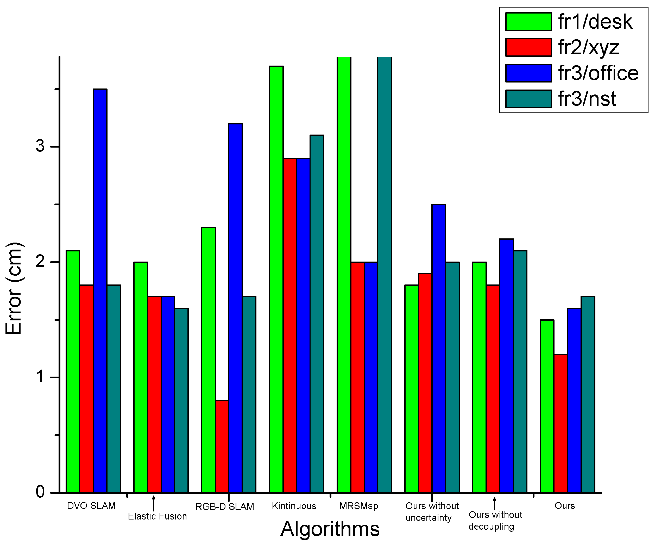
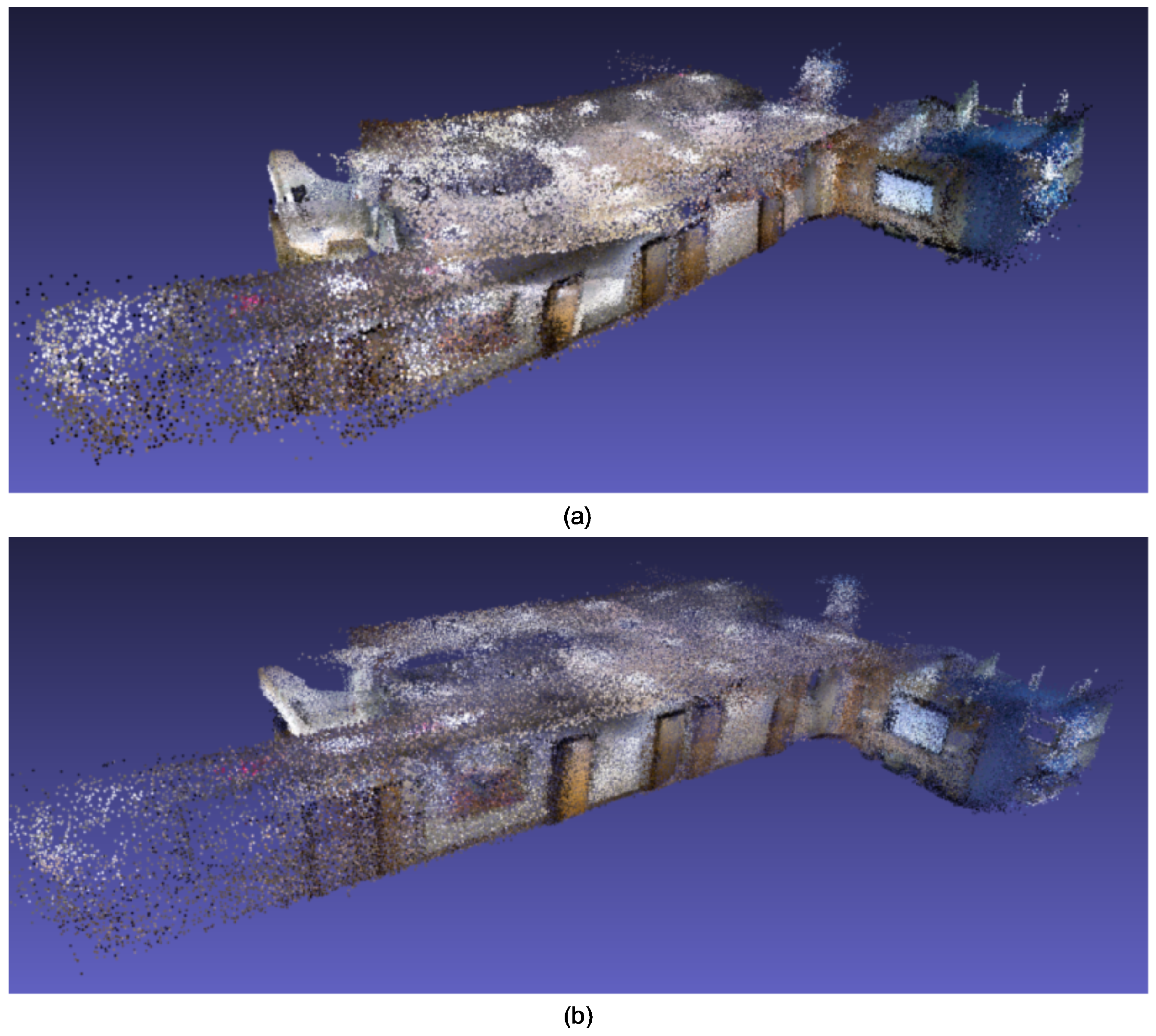
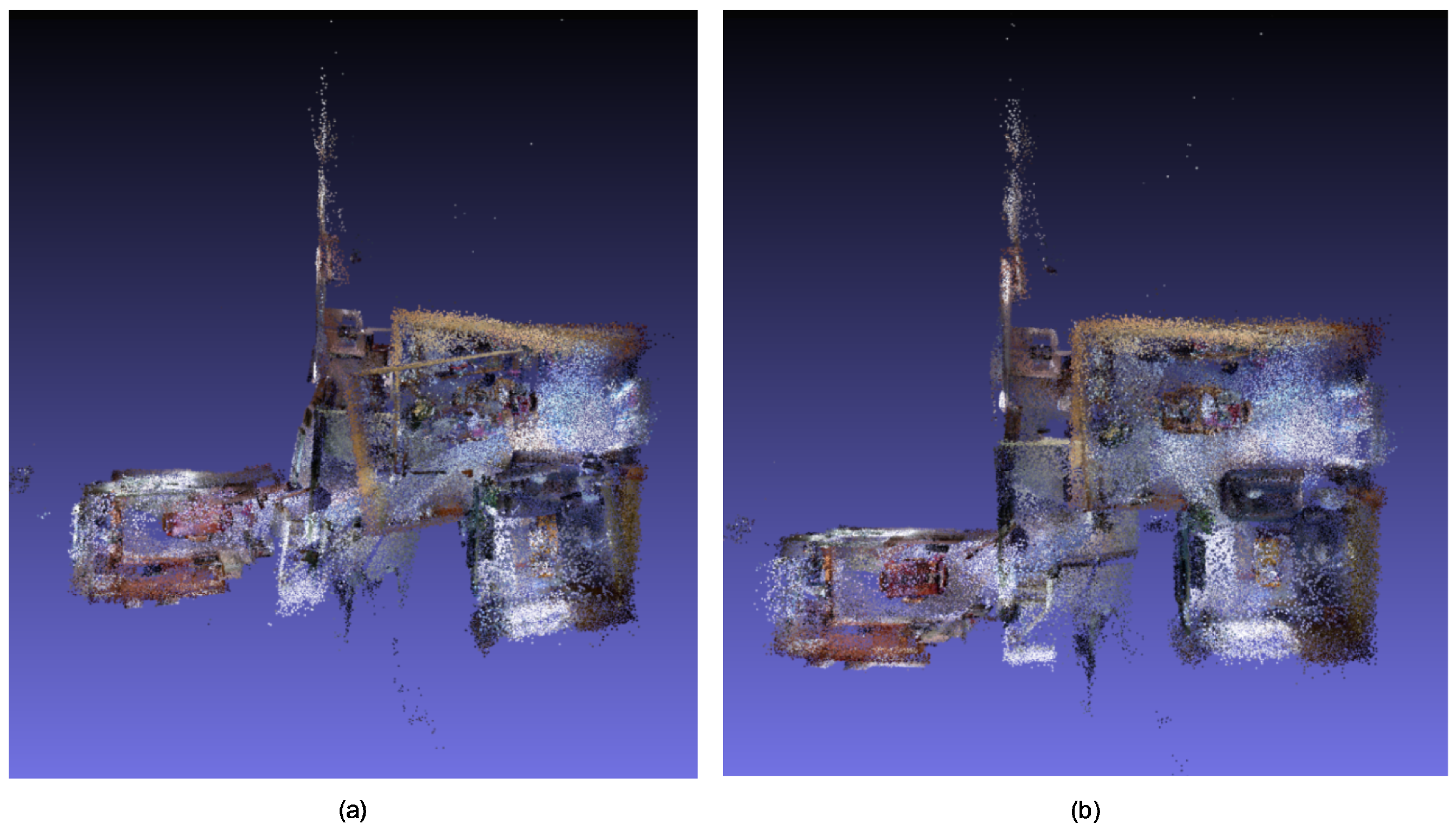
4. Experimental Section

The algorithm was evaluated over synthetic datasets and real datasets. The synthetic dataset was from the study [44]. In order to assess the quality of the camera pose estimation of the proposed algorithm, we compared the pose trajectory with other RGB-D SLAM algorithms on the TUM (Technical University of Munich) dataset [45], which provided the ground truth trajectories. We also tested the algorithm on different indoor environments, for example a long corridor, a lab room, and a living room.

Firstly, we evaluated the proposed algorithm on a synthetic dataset [44]. As shown in Figure 5, the left figures are two RGB color images, and the right ones are two depth images. These images were randomly selected from about 1000 image pairs in the dataset. The synthetic dataset consisted of RGB and depth images obtained from camera trajectories in ray-traced 3D models in POVRay (Persistence of Vision Raytracer). We can see from the depth images that the noise around edges was very large, and cannot be ignored with respect to the 3D reconstruction data source.

We projected the depth image into 3D space, as shown in Figure 6a. Figure 6b presents the uncertainty model using the algorithm in Section 3.2. We can see that our uncertainty model can describe the spatial layout of noise, which has a high value on object edges. To make the algorithm more robust, the weights should be set to small values when the uncertainty is significant.

Figure 7 shows the 3D model from our algorithm and also a 3D model from the algorithm proposed in [35]. We can compare the two results with more details in Figure 8.

For a better evaluation of the estimated poses of the camera, we validated our methods on the TUM dataset, which scanned a small environment with an external device mounted on the Kinect camera. The device captures the pose of the camera with a very high accuracy and thus can be regarded as the ground truth in 3D reconstruction evaluations. We compared the result with different RGB-D SLAM algorithms and off-line RGB-D 3D reconstruction methods. As shown in Figure 9, our methods perform well on most of the sequences.

We also tested our methods without the uncertainty module, and the result were poor, as the wrong measurements contributed more to the object functions. The proposed method relies only on color images and decouples rotation estimations, which makes the result more robust over noisy sequences.

To validate the robustness of our method, we adopted an artificial noise generation method from [44]. As the TUM dataset provided the trajectory ground truth, we selected the fr3/nst dataset to perform the experiments. We increased the noise level incrementally and ran the algorithm five times to obtain the mean error. The results are presented in

Table 2. Robust comparison using artificial noise. We compare the trajectory results from our methods and Xiao et al. [35] when increasing the artificial noise.

Noise Level u/Algorithm	0	0.01	0.02	0.03	0.04	0.05	0.06	0.07
Ours	1.8	1.9	1.9	2.2	2.2	2.2	2.1	2.1
Xiao [35]	2.3	2.6	3.1	3.7	4.4	5.4	6.3	7.9

. We conclude from the results that the performance of the traditional bundle adjustment algorithm gradually became worse along with increasing noise. For our method, as the depth noise was described well by the noise model, the algorithm could detect the noise internally. The uncertainly of the pixel would be large if it contained much noise, that is to say, the information from these pixels was weak and, thus, would not affect the result significantly. The result of $u=0.06$ was even better than that of $u=0.05$, because when the uncertainty was too large, the pixel would be regarded as an outlier and not included in the optimization.

To test the general use of the algorithm, we conducted experiments on the dataset collected in different scenes. As shown in Figure 10a, a long corridor was scanned in about 2000 frames, and two results were compared using our methods and bundle adjustment [35]. We can clearly see that the methods of [35] suffered greatly from pose estimation errors, and our methods reconstructed the structure properties of the corridor. In another sequence, shown in Figure 11, the method [35] failed on the dataset, because there was so much noise on the depth images, and the optimization could easily converge to a local minimum without carefully considering the uncertainty. Our method can reconstruct these challenging scenes with the help of plane constraints.

5. Conclusions and Future Work

This paper presents a novel 3D reconstruction algorithm for the indoor environment using consumer RGB-D cameras. Though much progress in 3D reconstruction and structure from motion has been made in recent years, using a consumer camera to build a globally-consistent 3D map in a real-time manner is still challenging. Estimating every 6-DOF (Degree Of Freedom) pose for frames (or keyframes) is nontrivial, as the traditional bundle adjustment algorithm can easily become trapped in a local minimum solution, especially when dealing with a large amount of noise. We can easily obtain a locally-consistent 3D model, for example a 3D model for a cup, a desk or a sofa. However, it remains challenging to produce a globally-consistent 3D map without any human interaction. The depth image from the RGB-D camera is so noisy that we cannot ignore this fact.

The uncertainty model is important when we want to perform a large-scale 3D reconstruction, but not just for registering a few scans. Firstly, we analyzed the connections between the disparity values in the classical stereo camera model and the Kinect camera. We borrowed the study report about the simple point uncertainty and developed a new uncertainty model that takes the neighborhood pixels into consideration using Gaussian mixture and multi-windows. The new uncertainty model produced a better distribution of the noise when the environment was complex.

We observe that the rotation part in pose $SE\left(3\right)$ can be determined without the information from the depth image. Inspired by this, we proposed a novel algorithm to estimate the pose by decoupling the rotation and translation robustly. The rotation part was estimated using information from visual feature points of RGB images. The translation part was estimated using all the information from the depth images. Compared with traditional methods, which utilized the information on visual features (3D measure, $uv$ measure from color images, depth measure from depth image), our method was more robust, as it made use of more information and kept the rotation estimation from the noise of the depth measurement. Moreover, the optimization of the translation turned out to be a linear optimization problem that could be solved in a closed-form fashion, without worries about local minima and very fast to solve. Our optimization is performed on the Lie group $SO\left(3\right)$, which converges quickly, and there is no issue regarding singularity, which is a problem in Euler angle parametrization.

In the experiment, we validated our algorithm using many scenes, including simulation datasets, real datasets, and validation datasets with ground truth poses. Comparisons were performed both in the estimation of camera poses and also the 3D model of the environment. The results showed that our algorithm greatly improved accuracy and robustness and could provide a globally-consistent 3D map in the indoor environment.

The combination of indoor and outdoor maps is another promising direction in GIS applications. For now, the frameworks of these two are different, as indoor environments are stand-alone spaces, and it is difficult to combine them under the same coordinate system. With increasing numbers of indoor maps becoming available, an integrated framework can be proposed to combine all of this information. The spatial model, map maintenance, spatial index, and data management in the outdoor case could be adjusted to fit the scenarios in the indoor environment. Generalized, real-time, dynamic, positioning and navigation services may be provided in both indoor and outdoor environments in an integrated GIS system.

References

1. Hijazi, I.H.; Ehlers, M.; Zlatanova, S. NIBU: A new approach to representing and analysing interior utility networks within 3D geo-information systems. Int. J. Digit. Earth 2012, 5, 22–42. [Google Scholar] [CrossRef]
2. Thill, J.C.; Dao, T.H.D.; Zhou, Y. Traveling in the three-dimensional city: Applications in route planning, accessibility assessment, location analysis and beyond. J. Transp. Geogr. 2011, 19, 405–421. [Google Scholar] [CrossRef]
3. Loch-Dehbi, S.; Dehbi, Y.; Plümer, L. Estimation of 3D Indoor Models with Constraint Propagation and Stochastic Reasoning in the Absence of Indoor Measurements. ISPRS Int. J. Geo-Inf. 2017, 6, 90. [Google Scholar] [CrossRef]
4. Sternberg, H.; Keller, F.; Willemsen, T. Precise indoor mapping as a basis for coarse indoor navigation. J. Appl. Geodesy 2013, 7, 231–246. [Google Scholar] [CrossRef]
5. Kang, H.K.; Li, K.J. A Standard Indoor Spatial Data Model—OGC IndoorGML and Implementation Approaches. ISPRS Int. J. Geo-Inf. 2017, 6, 116. [Google Scholar] [CrossRef]
6. Atila, U.; Karas, I.; Turan, M.; Rahman, A. Automatic generation of 3D networks in CityGML and design of an intelligent individual evacuation model for building fires within the scope of 3D GIS. In Innovations in 3D Geo-Information Sciences; Springer: Berlin, Germany, 2014; pp. 123–142. [Google Scholar]
7. Zhang, L.; Wang, Y.; Shi, H.; Zhang, L. Modeling and analyzing 3D complex building interiors for effective evacuation simulations. Fire Saf. J. 2012, 53, 1–12. [Google Scholar] [CrossRef]
8. Biljecki, F.; Stoter, J.; Ledoux, H.; Zlatanova, S.; Çöltekin, A. Applications of 3D city models: State of the art review. ISPRS Int. J. Geo-Inf. 2015, 4, 2842–2889. [Google Scholar] [CrossRef] [Green Version]
9. Yeh, M.; Chou, Y.; Yang, L. The Evaluation of GPS techniques for UAV-based Photogrammetry in Urban Area. Int. Arch. Photogramm. Remote Sens. Spat. Inf. Sci. 2016, 41. [Google Scholar] [CrossRef]
10. Endres, F.; Hess, J.; Engelhard, N.; Sturm, J.; Cremers, D.; Burgard, W. An evaluation of the RGB-D SLAM system. In Proceedings of the 2012 IEEE International Conference on Robotics and Automation (ICRA), Saint Paul, MN, USA, 14–18 May 2012; IEEE: Piscataway, NJ, USA, 2012; pp. 1691–1696. [Google Scholar]
11. Newcombe, R.A.; Izadi, S.; Hilliges, O.; Molyneaux, D.; Kim, D.; Davison, A.J.; Kohi, P.; Shotton, J.; Hodges, S.; Fitzgibbon, A. KinectFusion: Real-time dense surface mapping and tracking. In Proceedings of the 2011 10th IEEE International Symposium on Mixed and Augmented Reality (ISMAR), Basel, Switzerland, 26–29 October 2011; IEEE: Piscataway, NJ, USA, 2011; pp. 127–136. [Google Scholar]
12. Whelan, T.; Kaess, M.; Johannsson, H.; Fallon, M.; Leonard, J.J.; McDonald, J. Real-time large-scale dense RGB-D SLAM with volumetric fusion. Int. J. Robot. Res. 2015, 34, 598–626. [Google Scholar] [CrossRef]
13. Litomisky, K. Consumer RGB-D Cameras and Their Applications; Rapport Technique; University of California: Oakland, CA, USA, 2012; Volume 20. [Google Scholar]
14. Khoshelham, K.; Elberink, S.O. Accuracy and resolution of kinect depth data for indoor mapping applications. Sensors 2012, 12, 1437–1454. [Google Scholar] [CrossRef] [PubMed]
15. Henry, P.; Krainin, M.; Herbst, E.; Ren, X.; Fox, D. RGB-D mapping: Using Kinect-style depth cameras for dense 3D modeling of indoor environments. Int. J. Robot. Res. 2012, 31, 647–663. [Google Scholar] [CrossRef]
16. Chen, K.; Lai, Y.K.; Hu, S.M. 3D indoor scene modeling from RGB-D data: A survey. Comput. Vis. Media 2015, 1, 267–278. [Google Scholar] [CrossRef]
17. Dai, A.; Nießner, M.; Zollhöfer, M.; Izadi, S.; Theobalt, C. BundleFusion: Real-time Globally Consistent 3D Reconstruction using On-the-fly Surface Reintegration. ACM Trans. Graph. (TOG) 2017, 36, 24. [Google Scholar] [CrossRef]
18. Haene, C.; Zach, C.; Cohen, A.; Pollefeys, M. Dense Semantic 3D Reconstruction. IEEE Trans. Pattern Anal. Mach. Intell. 2016, 39, 1730–1743. [Google Scholar] [CrossRef] [PubMed]
19. Dos Santos, D.R.; Basso, M.A.; Khoshelham, K.; de Oliveira, E.; Pavan, N.L.; Vosselman, G. Mapping indoor spaces by adaptive coarse-to-fine registration of RGB-D data. IEEE Geosci. Remote Sens. Lett. 2016, 13, 262–266. [Google Scholar] [CrossRef]
20. Khoshelham, K.; Dos Santos, D.; Vosselman, G. Generation and weighting of 3D point correspondences for improved registration of RGB-D data. Proc. ISPRS Ann. Photogramm. Remote Sens. Spat. Inf. Sci. 2013, 5, 127–132. [Google Scholar] [CrossRef]
21. Chow, J.C.; Lichti, D.D.; Hol, J.D.; Bellusci, G.; Luinge, H. Imu and multiple RGB-D camera fusion for assisting indoor stop-and-go 3D terrestrial laser scanning. Robotics 2014, 3, 247–280. [Google Scholar] [CrossRef]
22. Pavan, N.L.; dos Santos, D.R. A Global Closed-Form Refinement for Consistent TLS Data Registration. IEEE Geosci. Remote Sens. Lett. 2017, 14, 1131–1135. [Google Scholar] [CrossRef]
23. Pathak, K.; Birk, A.; Vaskevicius, N.; Pfingsthorn, M.; Schwertfeger, S.; Poppinga, J. Online three-dimensional SLAM by registration of large planar surface segments and closed-form pose-graph relaxation. J. Field Robot. 2010, 27, 52–84. [Google Scholar] [CrossRef]
24. Theiler, P.W.; Wegner, J.D.; Schindler, K. Globally consistent registration of terrestrial laser scans via graph optimization. ISPRS J. Photogramm. Remote Sens. 2015, 109, 126–138. [Google Scholar] [CrossRef]
25. Borrmann, D.; Elseberg, J.; Lingemann, K.; Nüchter, A.; Hertzberg, J. Globally consistent 3D mapping with scan matching. Robot. Auton. Syst. 2008, 56, 130–142. [Google Scholar] [CrossRef]
26. Lu, F.; Milios, E. Globally consistent range scan alignment for environment mapping. Auton. Robots 1997, 4, 333–349. [Google Scholar] [CrossRef]
27. Moulon, P.; Monasse, P.; Marlet, R. Global fusion of relative motions for robust, accurate and scalable structure from motion. In Proceedings of the IEEE International Conference on Computer Vision, Sydney, NSW, Australia, 1–8 December 2013; pp. 3248–3255. [Google Scholar]
28. Reich, M.; Yang, M.Y.; Heipke, C. Global robust image rotation from combined weighted averaging. ISPRS J. Photogramm. Remote Sens. 2017, 127, 89–101. [Google Scholar] [CrossRef]
29. Whelan, T.; Kaess, M.; Fallon, M.; Johannsson, H.; Leonard, J.; McDonald, J. Kintinuous: Spatially Extended KinectFusion; MIT-CSAIL-TR-2012-020; DSpace@MIT: Sydney, Australia, 9 July 2012. [Google Scholar]
30. Mur-Artal, R.; Tardós, J.D. ORB-SLAM2: An Open-Source SLAM System for Monocular, Stereo, and RGB-D Cameras. IEEE Trans. Robot. 2017. [Google Scholar] [CrossRef]
31. Concha, A.; Civera, J. RGBDTAM: A Cost-Effective and Accurate RGB-D Tracking and Mapping System. arXiv, 2017; arXiv:1703.00754. [Google Scholar]
32. Angeli, A.; Filliat, D.; Doncieux, S.; Meyer, J.A. Fast and incremental method for loop-closure detection using bags of visual words. IEEE Trans. Robot. 2008, 24, 1027–1037. [Google Scholar] [CrossRef] [Green Version]
33. Whelan, T.; Salas-Moreno, R.F.; Glocker, B.; Davison, A.J.; Leutenegger, S. ElasticFusion: Real-time dense SLAM and light source estimation. Int. J. Robot. Res. 2016, 35, 1697–1716. [Google Scholar] [CrossRef]
34. Hou, Y.; Zhang, H.; Zhou, S. Convolutional neural network-based image representation for visual loop closure detection. In Proceedings of the 2015 IEEE International Conference on Information and Automation, Lijiang, China, 8–10 August 2015; IEEE: Piscataway, NJ, USA, 2015; pp. 2238–2245. [Google Scholar]
35. Xiao, J.; Owens, A.; Torralba, A. Sun3d: A database of big spaces reconstructed using sfm and object labels. In Proceedings of the IEEE International Conference on Computer Vision, Sydney, NSW, Australia, 1–8 December 2013; pp. 1625–1632. [Google Scholar]
36. Halber, M.; Funkhouser, T. Fine-To-Coarse Global Registration of RGB-D Scans. In Proceedings of the IEEE Conference on Computer Vision and Pattern Recognition, Honolulu, HI, USA, 21–26 July 2017. [Google Scholar]
37. Vestena, K.; Dos Santos, D.; Oilveira, F., Jr.; Pavan, N.; Khoshelham, K. A Weighted Closed-Form Solution for RGB-D Data Registration. In Proceedings of the 2016 23th ISPRS Congres, the International Archives of the Photogrammetry, Remote Sensing and Spatial Information Sciences, Prague, Czech Republic, 12–19 July 2016. [Google Scholar]
38. Oehler, B.; Stueckler, J.; Welle, J.; Schulz, D.; Behnke, S. Efficient multi-resolution plane segmentation of 3D point clouds. In Proceedings of the 4th International Conference on Intelligent Robotics and Applications, Aachen, Germany, 6–8 December 2011; pp. 145–156. [Google Scholar]
39. Lowe, D.G. Object recognition from local scale-invariant features. In Proceedings of the Seventh IEEE International Conference on Computer Vision, Kerkyra, Greece, 20–27 September 1999; IEEE: Piscataway, NJ, USA, 1999; Volume 2, pp. 1150–1157. [Google Scholar]
40. Bay, H.; Tuytelaars, T.; Van Gool, L. Surf: Speeded up robust features. In Proceedings of the Computer vision–ECCV 2006, Graz, Austria, 7–13 May 2006; Springer: Berlin/Heidelberg, Germany, 2006; pp. 404–417. [Google Scholar]
41. Rublee, E.; Rabaud, V.; Konolige, K.; Bradski, G. ORB: An efficient alternative to SIFT or SURF. In Proceedings of the 2011 IEEE international conference on Computer Vision (ICCV), Barcelona, Spain, 6–13 November 2011; IEEE: Piscataway, NJ, USA, 2011; pp. 2564–2571. [Google Scholar]
42. Hartley, R.; Zisserman, A. Multiple View Geometry in Computer Vision; Cambridge University Press: Cambridge, UK, 2003. [Google Scholar]
43. Rusu, R.B.; Blodow, N.; Marton, Z.C.; Beetz, M. Close-range Scene Segmentation and Reconstruction of 3D Point Cloud Maps for Mobile Manipulation in Domestic Environments. In Proceedings of the 2009 IEEE/RSJ International Conference on Intelligent Robots and Systems, St. Louis, MO, USA, 10–15 October 2009; IEEE: Piscataway, NJ, USA, 2009; pp. 1–6. [Google Scholar]
44. Handa, A.; Whelan, T.; McDonald, J.; Davison, A.J. A benchmark for RGB-D visual odometry, 3D reconstruction and SLAM. In Proceedings of the 2014 IEEE International Conference on Robotics and Automation (ICRA), Hong Kong, China, 31 May–7 June 2014; IEEE: Piscataway, NJ, USA, 2014; pp. 1524–1531. [Google Scholar]
45. Sturm, J.; Engelhard, N.; Endres, F.; Burgard, W.; Cremers, D. A Benchmark for the Evaluation of RGB-D SLAM Systems. In Proceedings of the 2012 IEEE/RSJ International Conference on Intelligent Robot Systems (IROS), Vilamoura, Portugal, 7–12 October 2012. [Google Scholar]
46. Kerl, C.; Sturm, J.; Cremers, D. Dense visual SLAM for RGB-D cameras. In Proceedings of the 2013 IEEE/RSJ International Conference on Intelligent Robots and Systems (IROS), Tokyo, Japan, 3–7 November 2013; IEEE: Piscataway, NJ, USA, 2013; pp. 2100–2106. [Google Scholar]
47. Stückler, J.; Behnke, S. Model Learning and Real-Time Tracking using Multi-Resolution Surfel Maps. In Proceedings of the AAAI Conference on Artificial Intelligence (AAAI-12), Toronto, ON, Canada, 22–26 July 2012. [Google Scholar]
Figure 1. Overview of the proposed algorithm.
Ijgi 06 00323 g001
Figure 2. Feature extraction using ORB on two frames. (a) An RGB image from the first frame; (b) an RGB image from the second frame; (c) feature matching result using ORB descriptors and (d) feature matching refined using RANSAC.
Ijgi 06 00323 g002
Figure 3. Camera model comparison between the stereo camera and the RGB-D camera. (a) A standard stereo camera. The subscripts r denotes the right camera, and l denotes the left one; (b) an RGB-D camera. There is another virtual reference plane beyond the object plane.
Ijgi 06 00323 g003
Figure 4. The uncertainty model developed in our algorithm. (a) An RGB image from the camera; (b) a depth image from the camera; (c) a result from the uncertainty model using independent pixel methods; (d) a result from the uncertainty model using our method.
Ijgi 06 00323 g004
Figure 5. Sample RGB image and depth image from the dataset [44]. (a) and (c) RGB images; (b) and (d) depth images.
Ijgi 06 00323 g005
Figure 6. Uncertainty model applied to the depth image. (a) Point cloud from the original depth image and (b) the uncertainty map.
Ijgi 06 00323 g006
Figure 7. 3D reconstruction result comparison with bundle adjustment [35]. (a) 3D model from [35]; (b) 3D model from the proposed method.
Ijgi 06 00323 g007
Figure 8. Detailed 3D reconstruction result comparison with bundle adjustment [35]. (a,b) Details of the 3D model from [35]; (c,d) details of the 3D model from the proposed method.
Ijgi 06 00323 g008
Figure 9. The RMSE of the absolute trajectory error (cm) of our proposed algorithm in comparison to previous methods on the TUM datasets of [10]. The algorithms from left to right are: DVO SLAM [46], Elastic Fusion [33], RGB-D SLAM [10], Kintinuous [29], MRSMap [47] and ours.
Ijgi 06 00323 g009
Figure 10. Test result using a corridor environment with multiple rooms. (a) Traditional BA [35] cannot recover the whole structure of the corridor environment; (b) the proposed method produced a good 3D model for this environment.
Ijgi 06 00323 g010
Figure 11. Test result using a typical house environment. (a) Traditional BA [35] suffers from the noisy data source and produces a rough 3D model; (b) the proposed method produced a 3D model fitting to the structure of the environment.
Ijgi 06 00323 g011