1. Introduction
Landslides are common geological disasters in mountainous areas that cause considerable economic and ecological damage. Many countries and regions suffer from landslides; for example, because of the complex geographical conditions and expanding human activities, more than 20,000 landslides occur in China annually, leading to nearly 1000 deaths or missing people, and a direct economic loss of six billion dollars [
1,
2].
A landslide susceptibility map plays an essential role in urban and rural planning. A landslide susceptibility map (LSM) that emphasizes static landslide-prone conditions presents information on the spatial distribution and probability of landslides in a certain region. In addition, these maps can assist decision makers in risk mitigation, land use management, space development, and environmental conservation to succeed in optimal development [
3,
4]. Using a geographic information system (GIS), various methods have been proposed, which mainly include expert evaluation, statistical methods, and mechanical approaches [
5]. Expert evaluation depends on the judgment of experts, whereas mechanical approaches assess slope stability using deterministic methods and/or numerical methods with a high accuracy [
6,
7]. However, as they are limited by model selection and data acquisition, mechanical approaches are only applied to small regions and situations that require high accuracy. Compared with the abovementioned approaches, the statistical methods based on connections between influence factors and landslides, not only avoid the dependence of mechanical models on high-precision data, but also reduce the subjectivity brought by expert evaluation statistical methods [
8,
9]. The statistical methods include the weighted liner combination model (WLC) [
10,
11], the logistic regression model [
12,
13,
14], fuzzy synthetic evaluation model [
15,
16], and neural network model [
17,
18].
Previous studies have shown that data processing and the weight of influence factors are the key components when applying statistical methods to landslide susceptibility mapping [
19]. Recently, Wang et al. (2016) [
20] took the statistical index curve and Zhang et al. (2014) [
21] utilized the cumulative frequency curve to classify influence factors for data processing; however, different X-axis intervals may affect the distribution of graphic features and result in different classifications. Meanwhile, buffers are built to consider the influence of locational elements on landslides in GIS analyses, and there is a need to determine buffer length thresholds before building them. Since there are no universal criteria or guidelines, scholars prefer to utilize subjective methods as a solution to this issue. Various weighting methods can be used in regional landslide susceptibility mapping. One commonly-used method is the analytical hierarchy processes (AHP) that is considered as a decision-aiding method for handing multi-criteria decisions [
22,
23,
24,
25]. However, the AHP method has some limitations [
3,
26], one of which is its inability to characterize the importance of each influence factor in different locations. For instance, if a mapping cell is far away from a locational element, the influence of this locational factor on landslides is negligible, leading to dimension changes in the preference matrix, and the constant weights calculated using the AHP method cannot deal with this issue well.
For these reasons, K-means clustering and binarization were introduced for data processing. Considering the different locations of mapping cells, the variable-weighted method was established based on the AHP method. On this basis, the variable-weighted linear combination model was established and applied to regional landslide susceptibility mapping for the Shennongjia Forestry District, China.
2. Study Area and Data Used
2.1. Study Area
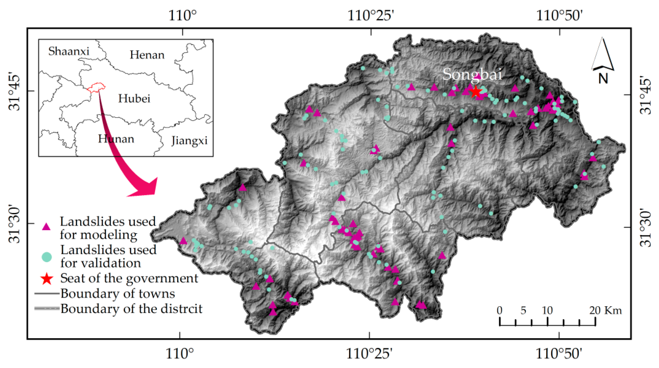
The Shennongjia Forestry District is located within latitude 31°15′–31°75′ N and longitude 109°56′–110°58′ E in Northwest Hubei, China (
Figure 1). The total area is about 3250 km
2, and the population was 79,248 as of 2014. The district is bound by the Ta-pa Mountains, with altitudes ranging from 430 m to 3100 m. Located in the mid-latitude northern subtropical monsoon zone, the district has a slightly cool and rainy climate, an average annual temperature of 12 °C, and precipitation is mainly concentrated between May and October. The district also has a dense network of rivers. The main north–south travel route is China National Highway 209, and Hubei Provincial Route 307 runs through the northeastern part of the district. Houses, tourist attractions, and other buildings are widely distributed along the rivers and roads.
In recent years, with the expansion of human activities, landslides have occurred more and more frequently in this district. Among the existing landslides, shallow landslides have the most extensive distribution (almost 80% of the total landslides over the last decade), which pose serious threats to resident life and also restrict the economy. Therefore, it is necessary for decision makers to take into account susceptibility to shallow landslides during urban and rural planning.
2.2. Data Used
2.2.1. Landslide Inventory Map
Four different datasets were prepared for landslide susceptibility mapping (
Table 1). The first of these was a landslide inventory map. A landslide inventory map helps to analyze the connections between influence factors and landslides [
27,
28,
29,
30].
By means of extensive field surveys and spatial analysis using GIS, a digitized inventory map of the district was completed by the Land Resources Bureau of the Shennongjia Forestry District; from which relevant data regarding 199 shallow landslides were extracted. However, the original inventory map only presented the type, occurrence time, area, and location (central position). To get more attributes of the existing landslides, buffers were built with the landslide points as centers, the sizes of which were equal to the recorded areas of landslides. Then, using the zonal statistics tool of the mapping and analytics platform, ArcGIS 10.2 [
31], the averages within the buffers were extracted from the factor layers (elevation, gradient, etc.). On this basis, 127 landslides (64%) were used for modeling and the remaining 72 landslides (36%) were used for model validation.
2.2.2. Topographical Factors
The second dataset was the digital elevation model (DEM)-based dataset, including topographical factors [
32]: elevation, gradient, aspect, relief amplitude (RA), surface roughness (SR), plan curvature (PLC), and profile curvature (PRC). However, having more factors does not necessarily mean a more complete and accurate landslide susceptibility map [
13,
21,
33]. Due to being derived from the same DEM data source, the topographical factors were not independent of each other. To select suitable factors, correlations of topographical factors were analyzed using the Pearson correlation coefficient, which is the covariance of two variables divided by the product of their standard deviations:
where
n is the number of samples;
xi,
yi are the single samples indexed with
i;
is the sample mean of
xi;
is the sample mean of
yi;
sx is the sample standard deviation of
xi;
sy is the sample standard deviation of
yi. The R has a value between −1 and +1, where 1 is total positive linear correlation, 0 is no linear correlation, and −1 is total negative linear correlation.
Using the statistical analysis software, SPSS 22, the Pearson correlation coefficients of each topographical factor were calculated. As shown in
Table 2, the following pairwise sets of factors have relatively high correlations: Gradient with RA, gradient and SR, RA with SR, PLC with PRC. Therefore, to reduce correlations as much as possible, and to make the selected factors more universal, only elevation and gradients with
R = 0.08 were considered as influencing factors for landslide susceptibility mapping.
2.2.3. Locational Factors
The locational factors refer to the proximity to locational elements (road, river, and fault), and the maps of locational elements constituted the third dataset. Roads affect landslides in the form of slope cuts and barriers to surface flow [
34]. The influences of rivers on landslides are mainly manifested through scouring and changes of water level, which lead to a decline in support capacity. Land that is close to faults is considered to be relatively weak, with altered surface material structures and increased permeability [
19,
35].
2.2.4. Lithology, Aquifer Storage Capacity, Precipitation, and Land Use
The fourth dataset includes lithology, aquifer storage capacity, precipitation, and land use [
36,
37]. Variations of lithology lead to different resistances to erosion processes, due to varied characteristics, such as different composition, structure, and compactness [
38,
39,
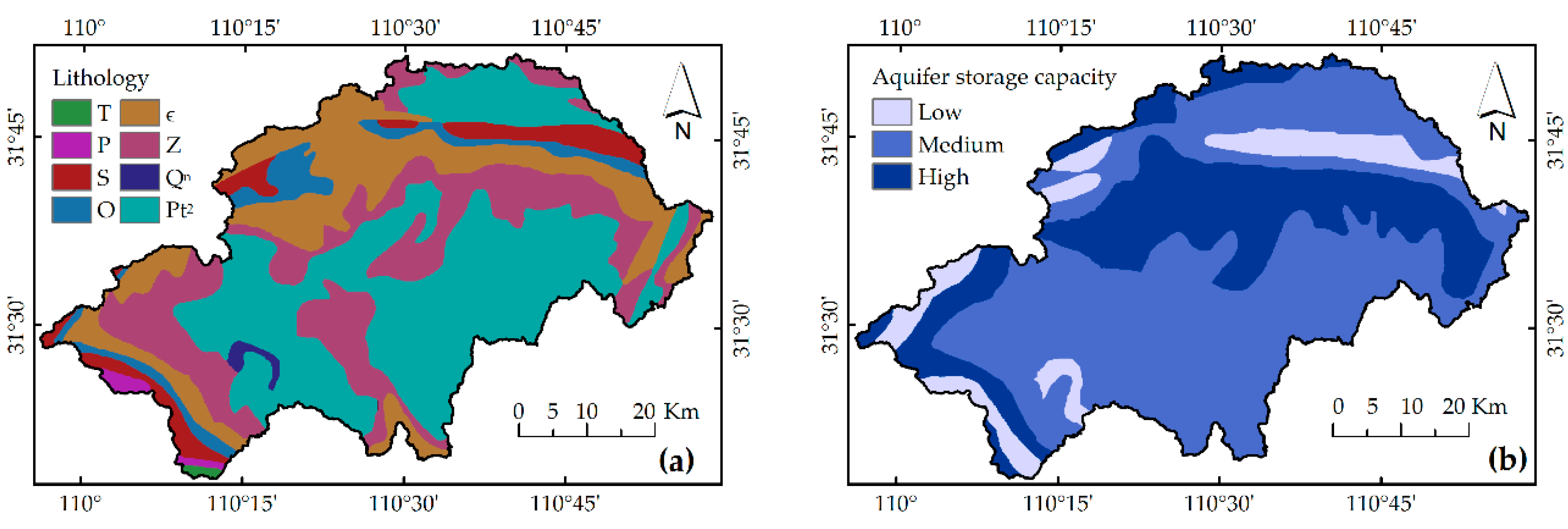
40]. The high storage capacity of aquifers can increase soil moisture and soften the structural plane of slopes, leading to a reduction in the original stability. For being directly digitized from public thematic maps, maps of lithology, aquifer storage capacity have been classified already: The lithology of the outcrop in the district has been classified into nine categories according to period: Triassic (
T), Permian (
P), Silurian (
S), Ordovician (
O), Cambrian (ϵ), Sinian (
Z), Qingbaikouan (
Qn), and Middle-Proterozoic (
Pt2) (
Figure 2a). Additionally, the aquifers have been classified into high, medium, and low, according to their relative storage capacities (
Figure 2b).
It is universally acknowledged that precipitation is the dominant exterior factor triggering landslides [
41,
42]. Using precipitation data from the last ten years, from eight meteorological observation stations in the district, a map of average annual precipitation was produced using the Kriging method, an interpolation method of ArcGIS 10.2. Different land-use types have different influences on the surrounding environment of slopes. The land of the district was classified into three main categories: Agricultural land, construction land, and unused land, based on Article Four of Land Administration Law of China (2004). Agricultural land had the largest proportion (98.68% of the total), which included forest land (92.5%), artificial forest land (2.93%), irrigation land (0.9%), etc., while unused land had the smallest (0.59%). The land use seemed to be uniform throughout the district; therefore, the land use was not selected as the influence factor.
3. Methodology
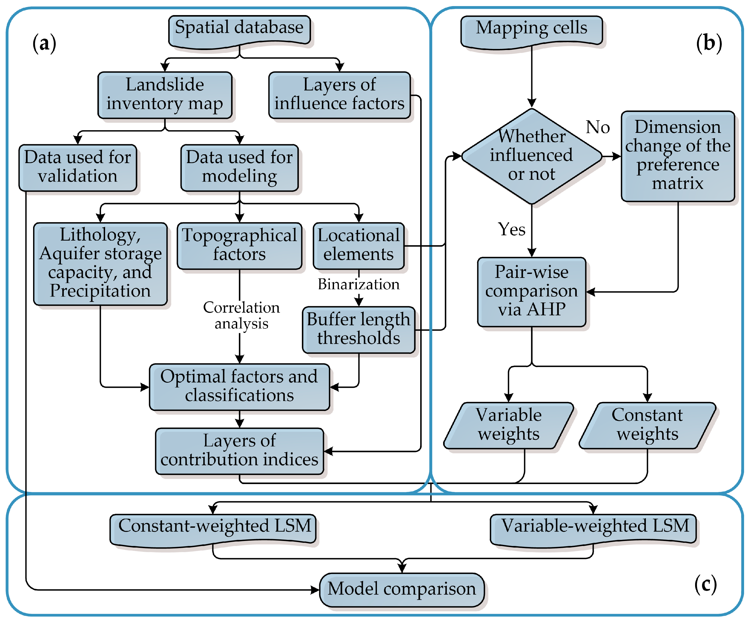
3.1. Weighted Linear Combination Model
The weighted linear combination model (WLC) is one of the most effective methods for landslide susceptibility mapping. WLC can transform multi-factor evaluation results into comprehensive ones through a linear superposition, according to the importance of each factor. The model is based on the following equation:
where
LSI is the landslide susceptibility index,
n is the total number of influence factors,
wi represents the weight of factor
i, and
ui represents the contribution index of factor
i.
The procedure of susceptibility mapping based on WLC can be divided into three steps: data processing, weighting, and mapping and model comparison (
Figure 3).
3.2. Classification
The classification of influence factors refers to a process by which a single factor is classified into secondary conditions. In this paper, lithology and aquifer storage capacity have been already classified as they were directly extracted from the original thematic maps; K-means clustering and binarization were introduced for data processing of the remaining selected factors.
3.2.1. K-Means Clustering
K-means clustering is a dynamic clustering method based on distance measurements, which is widely used in the fields of data exploration [
36,
43,
44]. K-means clustering takes the Euclidean distance as the similarity criterion and calculates the distance from sample
xi to each centroid,
uk, for a given database,
X = {
x1,
x2 …,
xn}, and a given number (
k) of clusters
C = {
c1,
c2 …,
ck}:
K-means uses an iterative algorithm to minimize the sum of point-to-centroid distances and sums over all
k clusters:
To verify the accuracy of the classification, the Tabular Accuracy Index (
TAI) [
45] was employed.
TAI refers to the ratio between the classification error and the “potential error” inherent to the unclassified data, which is a standardized measure of the data classification [
46]:
where
N is the total number of samples,
k is the number of clusters,
is the average of all the samples,
is the average of class
j, and
nj is the total number of classes
j. The
TAI values range from 0 to 1, and the higher the
TAI value is, the greater the accuracy of the classification.
3.2.2. Binarization
The distance data between the locational elements and the existing landslides are the basis for determining buffer length thresholds. However, the extreme data of distance, which reveals that a landslide is located far away from the elements, may create a larger threshold, leading to an increasing cost in the prevention and management of landslides. To eliminate these extreme data, binarization, commonly-used in field of image segmentation [
47,
48,
49], was introduced:
where
ui represents the binary value,
d represents the distance between the locational elements and existing landslide
i, and
L represents the maximum threshold.
Assuming that
(
i is the number of the iterations) divides the existing landslides (
C) into a part that is influenced by the locational elements (
) and a part that is not (
), the sum of point-to-centroid distances was calculated based on K-means clustering:
where
is the centroid of part
;
is the centroid of part
.
A minimum value of
J(C) identified the final centroid:
The average of the centroids ((u1 + u0)/2) was taken as the maximum buffer length threshold L. Then, the remaining distance data were classified by K-means to obtain other thresholds.
3.3. The Contribution Index
Instead of the commonly-used expert scores, landslide density
unum, and landslide area density
uarea were adopted as contribution indices of influence factors to reduce subjectivities [
50]:
where
Nij is the number of landslides in class
j of factor
i, and is analogous to
sij .
The larger coefficient of variation (CV), the more diversified the data and the more relevant the correlation, therefore CV was used to compare the dispersion degrees between the two indices for the suitable index selection [
51]. Additionally, the unit area index (
UAI) was introduced to characterize the average area of landslides in a certain class:
3.4. Variable-Weighted Method
AHP involves pair-wise comparisons of decision factors and provides a relative dominance value, ranging from one to nine, to calibrate the qualitative and quantitative performances of priorities [
52]. The consistency index is used to improve the consistency of judgments:
where
n is the number of factors and
is the maximum preference matrix eigenvalue.
The consistency ratio is used to verify whether the preference matrix is randomly generated:
where
RI is the random consistency index. A
CR value of less than 0.1 means a satisfactory consistency.
However, the influences of the factors on landslides differ with the locations of the mapping cells. For this reason, the variable-weighted method was established to determine the weight of each factor according to the locations of the mapping cells. The preference matrix can be established as the following equation:
where
n is the number of factors;
k is the number of locational factors,
n <
k;
m = 1, 2, ...,
n;
is the result of pair-wise comparison, and
.
If the mapping cell is located in a region where k locational factors are negligible, the combination of factors changes, leading to a dimension change of the preference matrix. It can be seen that the number of combination changes is .
4. Results
4.1. The Classification of Elevation, Gradient and Precipitation Using K-Means
Using K-means clustering, elevation, gradient, and precipitation were classified. As shown in
Table 3,
TAIs using K-means are generally higher than Jenks (an internal algorithm of ArcGIS 10.2), especially the
TAI of precipitation using K-means, which is 0.1 higher than the
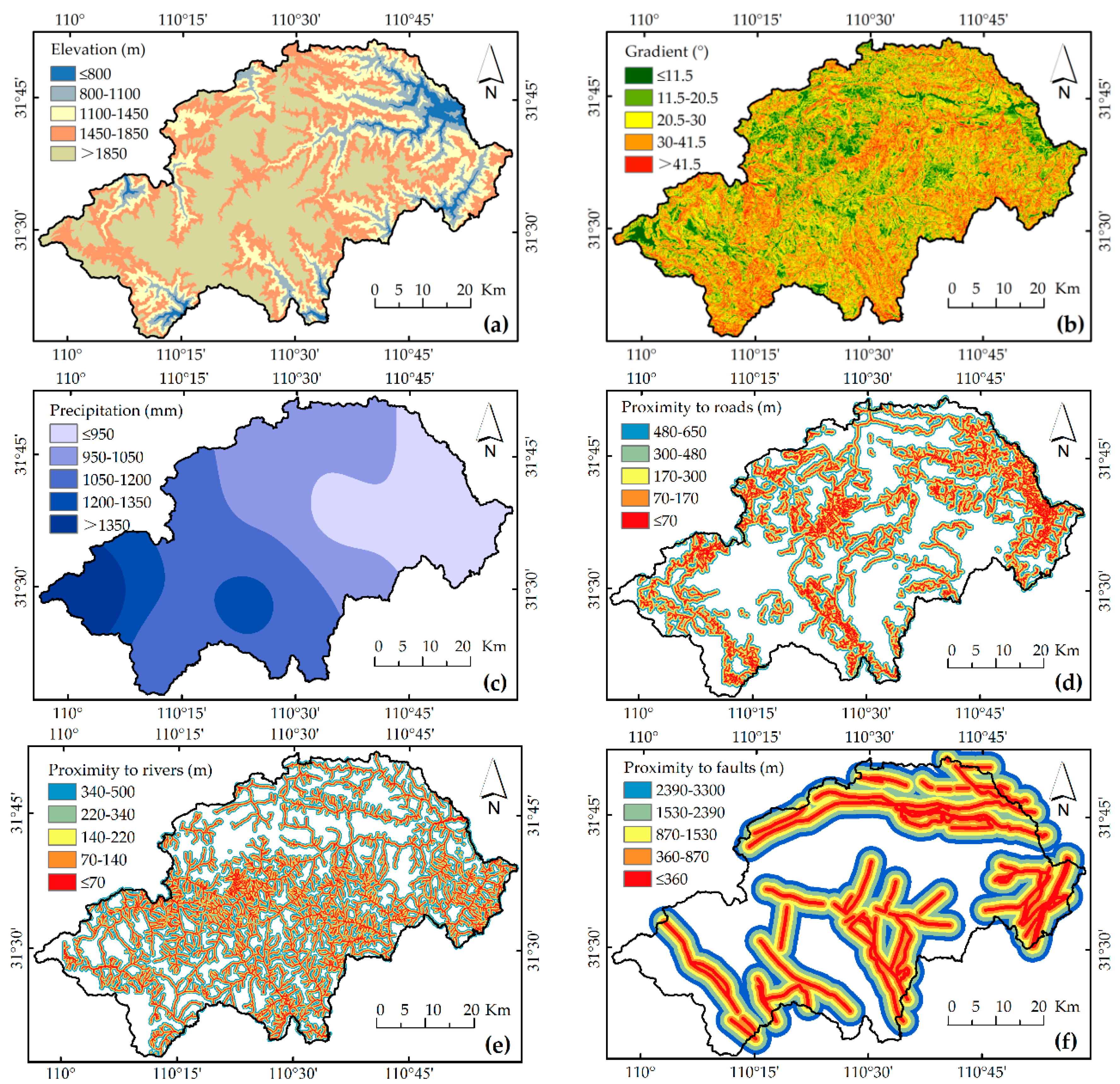
TAI using Jenks. Hence, the input layers of elevation, gradient, and precipitation were produced using the relevant class intervals in ArcGIS 10.2. (
Figure 4a–c).
4.2. The Building of Buffers by Binarization
Using binarization, the buffer length thresholds of locational elements were determined. The computation shows that the data of 13 landslides were eliminated using binarization, leading to a sharp decrease in the maximum threshold, from 19,650 m to 650 m, and also showed an increase in
TAI from 0.78 to 0.81 (
Table 4). The situations are the same for rivers and faults. Subsequently, the buffers were built with the relevant thresholds to consider the influence of locational factors. The obtained vector layers were converted into raster ones, with a cell size of 10 m, to be compatible with the spatial resolution (
Figure 4e–f).
4.3. Contrastive Analysis among the Contribution Indices
Landslide density (
unum), and landslide area density (
uarea) of each factor were calculated using Equations (9) and (10). As shown in
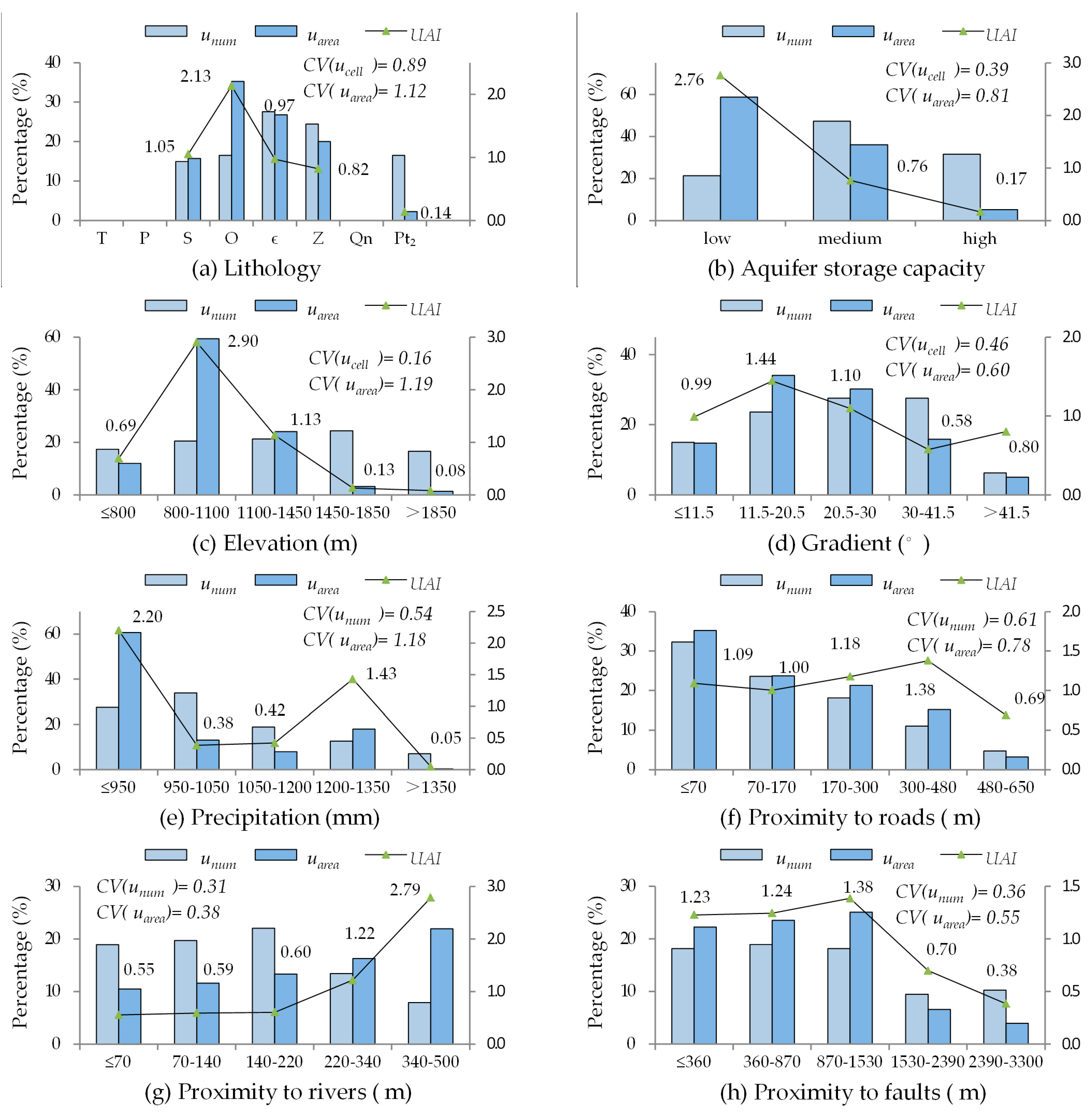
Figure 5a,
unum is evenly distributed along the elevations, and the greatest
uarea (59.34%) corresponded to an elevation range of 800–1100 m. The
CV of
uarea is far greater than that of
unum, which reveals that the contribution of the elevation range of 800–1100 m can be better-characterized by the greater dispersion of
uarea. Meanwhile, the distribution of the
UAI indicated that the unit area of landslides in the elevation range of 800–1100 m was greater than that of other elevations.
Figure 5d shows a different view: A greater gradient is not necessarily more prone to landslide occurances; the landslides were distributed in the gradient range of 0–41.5°. The distribution of the
UAI indicated that landslides with a greater area were concentrated in the gradient range of 11.5° to 30°, with the greatest
uarea being 64.28%. Aquifer storage capacity and precipitation had similar distributions (
Figure 5b,e). This is because regions with flat terrain and appropriate humidity are rare in the district, where the human activities are concentrated.
Figure 4c shows that Ordovician (
O) rock had the greatest
uarea (35.25%), and a relatively high
unum (16.54%), where landslides have a relatively greater unit area.
As shown in
Figure 5f, in the regions influenced by roads, with increasing distance from a road, the number of landslides decreases, while area increases. Although the
CVs of
unum and
uarea show little difference, both the indices showed that landslides are prone to occur in regions near roads.
Figure 5g shows that the
unum of proximity to rivers changes minimally within 0–220 m and then slowly decreases, while the
uarea continually increases with the increase in distance to a river. Regarding faults, the
unum and
uarea change minimally within the distance range of 0–1530 m and then slowly decrease (
Figure 5h).
It can be seen above that landslide area density
uarea can characterize the contribution of a certain class for having the greater
CVs. Therefore, landslide area density
uarea is more efficient for reflecting the connections between influence factors and landslides, and it was taken as the contribution index (
Table 5).
4.4. Weighting Using the Variable-Weighted Method
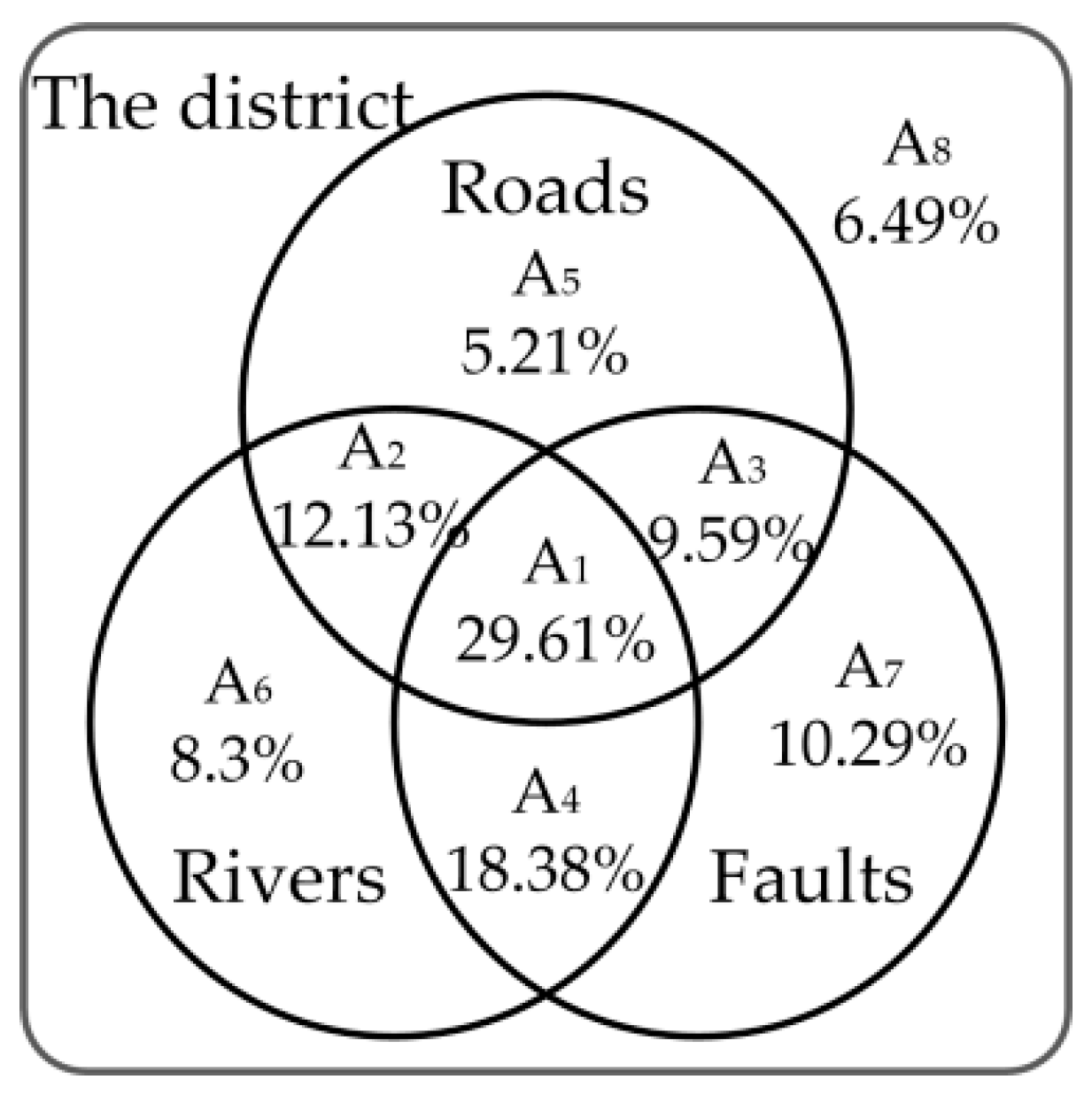
As shown in
Figure 6, the district was divided into eight different regions, according to whether the mapping cells were influenced by single or multiple locational elements. The regions where the traditional constant weights are applicable account for only 29.61% of the district. The weights of each factor were calculated using the variable-Weighted Method (
Table 6).
4.5. Landslide Susceptibility Mapping
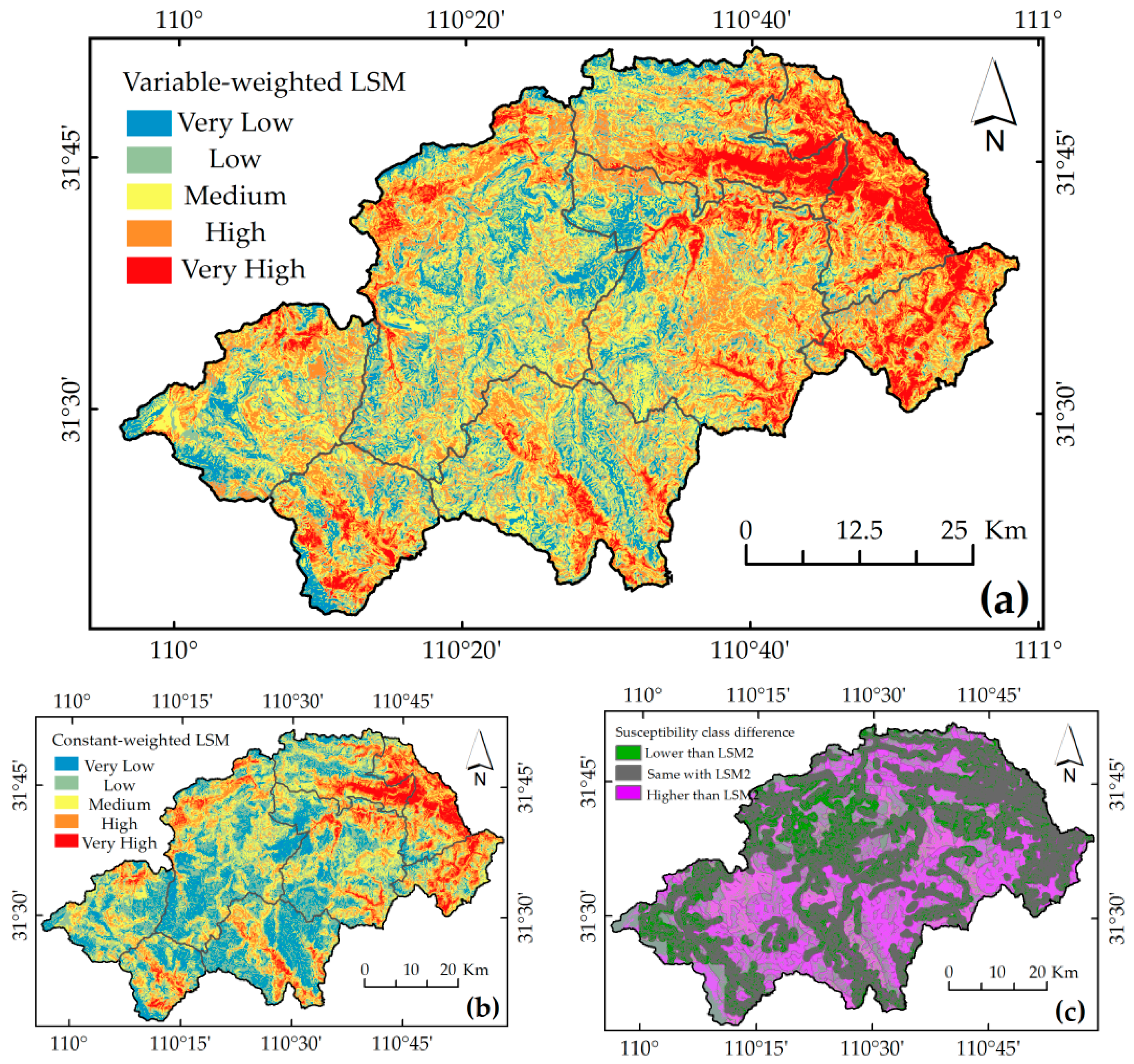
For landslide susceptibility mapping, the landslide susceptibility index was classified into five categories using K-means clustering: Very low (I), low (II), medium (III), high (IV), and very high (V). Subsequently, two landslide susceptibility maps were generated: (i) using variable weights (LSM1,
Figure 7a); and (ii) using constant weights (LSM2,
Figure 7b).
5. Discussion
There are two common features between the two different susceptibility maps: high and very high susceptible regions are located mainly in the northeast, where the gradient is gradual and the elevation is relatively low; and the high and very high susceptible regions are mainly distributed along roads, where the slope cuts and overloads may accelerate the instability of slopes.
It can be observed in
Figure 7a,b that more landslides occur in regions with the high and very high susceptibility class in LSM1: 59% of total number and 95.5% of the total area of the existing landslides are located in regions with high and very high susceptibility classes in LSM1, while 49.6% of total number and 93.5% of the total area of existing landslides are located in regions with high and very high susceptibility classes in LSM2.
As shown in
Figure 7c, 62.3% of the mapping cells have the same susceptibility class and are located in region A
1 where the influences of the three locational factors are considered. Meanwhile, 27% of the mapping cells have one susceptibility class higher than that of using the constant weights, and 0.56% of the mapping cells have two susceptibility classes higher than that of using the constant weights. Cells with higher susceptibility classes are mainly located in regions A
4, A
6, A
7, and A
8, where the influence of the roads is negligible. This is a fairly good result, which illustrates that the mapping cells may have high landslide susceptibility, even in the regions where the influence of the locational factor on landslides is negligible.
Hence, it is concluded that the landslide susceptibility map using the VWLC model has a higher accuracy and a more reasonable distribution of landslides.
6. Conclusions
Urban and rural planning is complex work that needs to take into account social, economic, and ecological factors. As for landslide-vulnerable regions, landslide susceptibility needs to be considered as well. An LSM could contribute to urban and rural planning, such as the movement and merger of villages, which can be planned by combining LSM with population distribution; based on LSM, in conjunction with the locations of infrastructure, property risk can be assessed.
In this paper, the variable-weighted linear combination model was established for the susceptibility mapping of shallow landslides, which mainly included the introduction of binarization for determining buffer length thresholds of the locational elements, and the establishment of the variable-weighted method for weighting, which takes different locations of mapping cells into consideration.
The introduction of binarization not only avoids the subjectivity brought by empirical judgments, but also reduces the effect of extreme values on buffer length thresholds. The maximum threshold of the proximity to roads in the district was 650 m, the maximum threshold of the proximity to rivers was 500 m, and the maximum threshold of the proximity to faults was 3300 m. The variable-weighted method considers the dimensional changes of the preference matrix varying with different locations of the mapping cells, and rationally evaluates susceptibility in regions where the influence of single or multiple locational factors is negligible.
Using the VWLC model and considering eight influence factors, elevation, gradient, precipitation, aquifer storage capacity, lithology, proximity to roads, proximity to rivers, and proximity to faults, a landslide susceptibility map for the Shennongjia Forestry District was produced. Compared with a susceptibility map using constant weights, the map based on VWLC was validated to have a higher accuracy and a more reasonable distribution of landslides.
Therefore, the VWLC model is more beneficial to urban and rural planning, and can be used for any location that has the same, or similar, geological and topographical conditions.


