Article

Evaluation of Feature Selection Methods for Object-Based Land Cover Mapping of Unmanned Aerial Vehicle Imagery Using Random Forest and Support Vector Machine Classifiers

1
Jiangsu Provincial Key Laboratory of Geographic Information Science and Technology, Nanjing University, Nanjing 210023, China
2
Department of Geoinformatics—Z_GIS, University of Salzburg, Hellbrunner Str. 34, A-5020 Salzburg, Austria
3
Urban and Resources Environmental College, Nanjing Second Normal University, Nanjing 210013, China
*
Author to whom correspondence should be addressed.
ISPRS Int. J. Geo-Inf. 2017, 6(2), 51; https://doi.org/10.3390/ijgi6020051
Submission received: 29 December 2016 / Revised: 10 February 2017 / Accepted: 15 February 2017 / Published: 18 February 2017

Abstract

:
The increased feature space available in object-based classification environments (e.g., extended spectral feature sets per object, shape properties, or textural features) has a high potential of improving classifications. However, the availability of a large number of derived features per segmented object can also lead to a time-consuming and subjective process of optimizing the feature subset. The objectives of this study are to evaluate the effect of the advanced feature selection methods of popular supervised classifiers (Support Vector Machines (SVM) and Random Forest (RF)) for the example of object-based mapping of an agricultural area using Unmanned Aerial Vehicle (UAV) imagery, in order to optimize their usage for object-based agriculture pattern recognition tasks. In this study, several advanced feature selection methods were divided into both types of classifiers (SVM and RF) to conduct further evaluations using five feature-importance-evaluation methods and three feature-subset-evaluation methods. A visualization method was used to measure the change pattern of mean classification accuracy with the increase of features used, and a two-tailed t-test was used to determine the difference between two population means for both repeated ten classification accuracies. This study mainly contribute to the uncertainty analysis of feature selection for object-based classification instead of the per-pixel method. The results highlight that the RF classifier is relatively insensitive to the number of input features, even for a small training set size, whereby a negative impact of feature set size on the classification accuracy of the SVM classifier was observed. Overall, the SVM Recursive Feature Elimination (SVM-RFE) seems to be an appropriate method for both groups of classifiers, while the Correlation-based Feature Selection (CFS) is the best feature-subset-evaluation method. Most importantly, this study verified that feature selection for both classifiers is crucial for the evolving field of Object-based Image Analysis (OBIA): It is highly advisable for feature selection to be performed before object-based classification, even though an adverse impact could sometimes be observed from the wrapper methods.

1. Introduction

Feature selection is considered an important step within a classification process because it improves the performance of the classifier and reduces the complexity of the computation by removing redundant information [1]. Feature selection has been widely applied in remote sensing image classification in general [2,3], and for hyperspectral data in particular [4,5]. With the extended feature space derived from segmented objects (e.g., extended spectral feature sets per object, shape properties, or textural features) [6,7], object-based classification may increase the complexity of the classification and the demand for computing power. An additional challenge is avoiding the time-consuming step of calculating all available features and the subjective process of artificial feature selection when determining optimal features, besides some other specific issues of object-based image analysis (e.g., object scale and training set size) [8,9].
Previous investigations have increasingly applied several advanced feature selection methods to object-based image analysis. Duro et al. [10] implemented feature selection by calculating the variable importance score using the Random Forest method. Stumpf and Kerle [11] and Puissant et al. [12] implemented an iterative backward elimination, whereby the least important 20% of variables, according to the variable ranking derived from the Random Forest method, were eliminated at each iteration to determine the optimal feature subset. The splitting rule for the decision tree was formerly used as the attribute selection measure [13] and has been used in several studies to train the decision tree model, while decision tree classifiers were widely applied to object-based image analysis [14,15]. For example, Vieira et al. [16] used the highest normalized information gain measure to select the attribute, and then selected the best model using cross-validation evaluation, while Peña-Barragán et al. [17] used the chi-square (χ2) statistic measure as the decision rule. Furthermore, Yu et al. [18] and Ma et al. [9] used the Correlation-based Feature Selection (CFS) method to implement dimensionality reduction of the object features prior to classification. Novack et al. [2] used four advanced feature selection algorithms to identify the most relevant features for the classification of a high-resolution image but did not further assess these methods and their respective performance relative to each other.
The above-mentioned studies consistently agree on the benefit (i.e., complexity reduction or accuracy improvement) of prior feature selection in object-based classification, but not all mentioned studies actually obtained an accuracy improvement, due to some fuzziness in object-based classification (e.g., the widespread usage of fuzzy classifiers and especially selection and parameterization of the segmentation methods as such). Furthermore, previous research for other high-dimensional data (e.g., hyperspectral data) revealed that parts of this uncertainty may be related to the effects of particular combinations of feature selection methods with different supervised classification methods [5,19]. Some studies claimed that SVM classifiers are insensitive to the dimensionality of the data-set [4,20,21], while Weston et al. [22] and Guyon et al. [23] observed an increase in classification accuracy through dimensionality reduction. From these somewhat contradictory findings, we may conclude that feature selection is predominantly regarded as having positive effects on the classification accuracy, but may cause a degree of uncertainty, particularly in SVM-based classifications. Similarly, studies on RF classifiers also yield some ambiguity regarding the effects of feature selection for object-based classification. This is important since, next to SVM, RF methods have gained popularity in object-based classification [11,12]. For example, Duro et al. [24] proved that RF with prior feature selection performed better than without feature selection, but Li et al. [19] suggested that RF is a stable object-based classification method with and without prior feature selection. In fact, Li et al. [19] never observed a statistically significant difference of classification accuracy between selected feature subsets and all features. Thus, it seems that feature selection in object-based classification reveals a research gap: There is no common consensus about the general effects of the combination of feature selection methods and object-based classification.
Image segmentation processes for the delineation of agriculture from Unmanned Aerial Vehicle (UAV) images have been in operational use for several years, e.g., for precision agriculture [25,26]. UAV images are usually different to other images (typically only RGB bands, very high spatial resolution, radiometric differences). Furthermore, due to laws and regulations, UAVs are mostly flown in areas without human presence (no urban areas) and where visual control is possible (open areas)—this results in an abundance of applications in agricultural areas compared to others. Subsequently, the ability to map agricultural areas at high spatial resolution encourages agriculture monitoring, combining UAV images with object-based methods, which contributes fundamental understanding to the available object-based classification methods.
This study mainly aims to analyze the uncertainty of various feature selection methods for object-based classification, instead of a similar evaluation for the per-pixel method. Based on the previous assessment of classification methods for agricultural areas using high-resolution images [19,24], this study now specifically focuses on assessing the effect of feature dimensionality and training set size on SVM and RF classifiers for different feature selection methods, including the filter method, wrappers, and embedded methods. The carefully designed assessment strategy provides new insight into the effect of different feature selection methods, and the statistical methods used assist in detecting the significant differences in mean classification accuracy. To our knowledge, this study is the first systematic evaluation of advanced feature selection methods in combination with the SVM and RF classifiers regarding object-based classification.

2. Methods

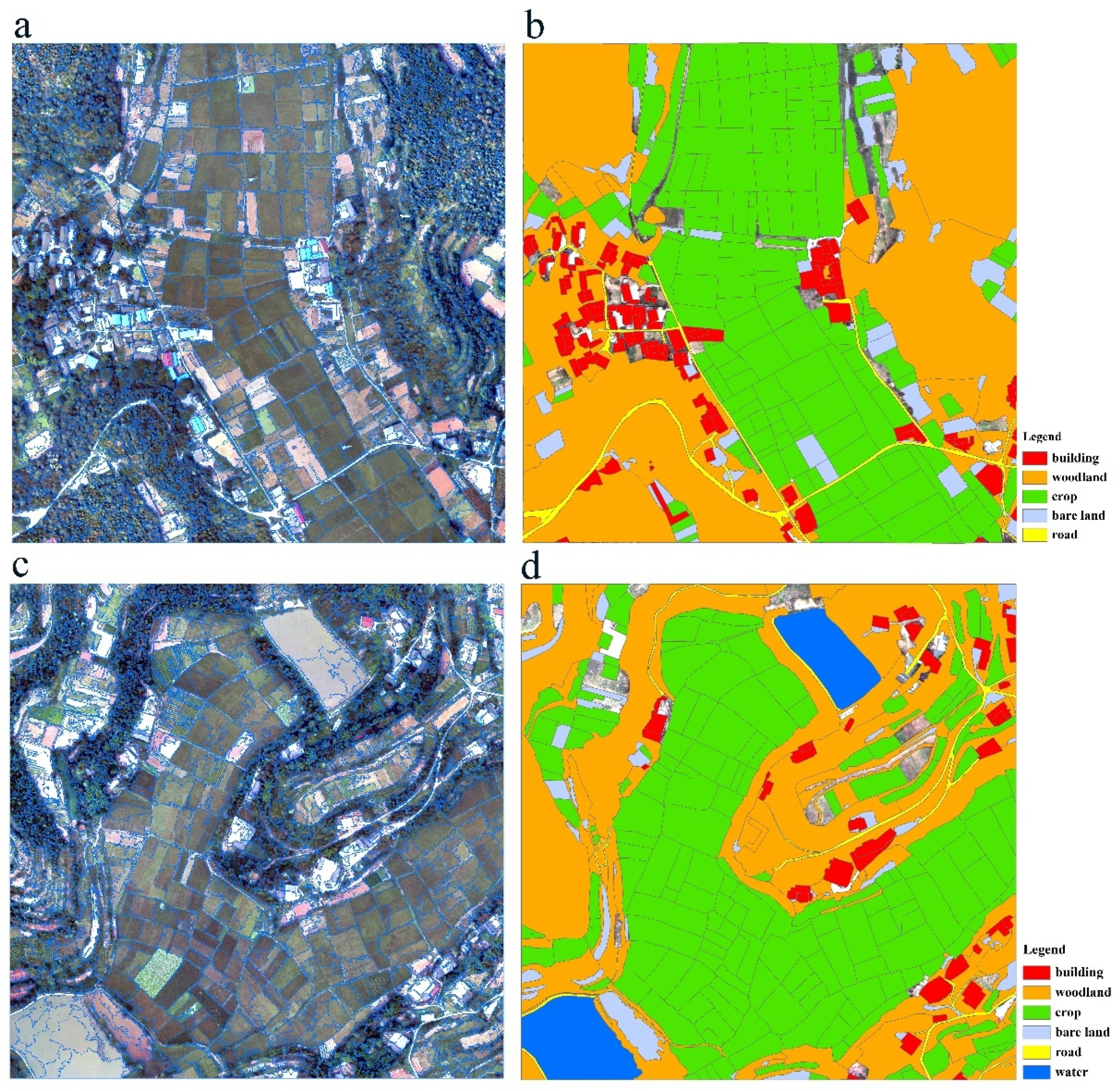
2.1. Study Area and Data Set

The study was conducted in the eastern suburbs of the city of Deyang, which is located in the Sichuan basin of China. The site extends approximately 10 × 5 km2, and land cover types are typically agricultural. In the study area, a UAV data set covering approximately 10 × 5 km2 was acquired with a Canon 5D 2 camera, at a height of around 750 m in August 2011. To subsequently produce a Digital Orthophoto Map (DOM), two standard map sheets of 500 × 500 m (0.2 m spatial resolution and RGB bands) were generated using digital photogrammetry software [27]. For the evaluation of feature selection methods, we selected both standard map sheets as study areas to enhance the results. Study area 1 (Figure 1a) mainly consists of cropland (38%) and woodland (43%), and also contains 6% buildings, 5% bare lands and 2% roads (Figure 1b). Study area 2 (Figure 1c) mainly comprises cropland (45%) and woodland (37%), and also contains 5% water, 4% buildings, 4% bare land, and 1% roads (Figure 1d). All percentages of the thematic classes were calculated using a reference layer derived from manual interpretation (see Figure 1b,d).

2.2. Segmentation and Features

The multi-resolution segmentation algorithm [28] implemented in the eCognition software package (Trimble Geospatial) was used to generate objects; the weights of colour and shape were set to 0.9/0.1, respectively, while those of smoothness/compactness were set to 0.5/0.5 (standard settings). The image (of which all three bands were weighted equally) was segmented at a medium scale parameter (homogeneity threshold) of 100, which was determined based on a previous classification assessment in terms of specific segmentation scale parameters [19]. 32 features were calculated within eCognition for each object, including spectral, texture and shape features, to subsequently implement in the feature selection algorithms.
The details of the selected features are given in Table 1. The spectral features comprised the mean and standard deviation of the object spectrum, along with the maximum difference and feature brightness. The shape measures consisted of the geometrical features provided by each segmented object, such as area, asymmetry, border index, compactness, density, elliptic fit, main direction, rectangular fit, shape index and roundness. The texture features of this study are based on the Haralick analysis (the gray-level co-occurrence matrix (GLCM) and gray-level difference vector (GLDV)) and are dependent upon all directions, namely, angle 2nd moment, contrast, correlation, dissimilarity, entropy, mean and standard deviation.

2.3. Feature Selection Algorithms

In this study, we implemented eight feature selection methods, including five filter methods (Gain ratio, Chi-square, SVM-RFE, CFS, and Relief-F), two wrapper methods (RF wrapper and SVM wrapper), and one embedded method (RF). We assessed the methods by dividing them into two categories according to the feature selection results (feature importance ranking and feature subset). All feature selection methods were integrated into a C# platform using version 3.7.9 of WEKA [29] or version 3.1.1 of R to be executed automatically.
(1) Gain ratio
The gain ratio is an extension of the information gain measure, which attempts to overcome the bias that the information gain measure is prone to selecting features with a large number of values [13]. Thereby, the information gain measure is used as an attribute selection measure of the decision tree and is obtained by computing the difference between the expected information requirement, classifying a tuple in tuples, and the new information requirement for attribute A after the partitioning. The measure of the expected information requirement is given by [13].
I n f o ( D ) = i = 1 m p i log 2 ( p i )
where m is the number of distinct classes; p i indicates the probability by calculating the proportion of belonging to class C i in tuples D. The new information requirement for attribute A is measured by
I n f o A ( D ) = j = 1 v | D j | | D | × I n f o ( D j )
where v indicates that D was divided into v partitions or subsets, { D 1 , D 2 , , D v } . Thus, the information gain measure Gain(A) for attribute A can be calculated by the formula.
Gain ( A ) = I n f o ( D ) I n f o A ( D )
Then, a ‘split information’ function was used to normalize the information gain measure Gain ( A ) . The split information function was defined by
S p l i t I n f o A ( D ) = j = 1 v | D j | | D | × log 2 ( | D j | | D | )
Finally, the gain ratio is calculated as the information gain measure Gain ( A ) divided by the split information measure S p l i t I n f o ( A ) , that is
G a i n R a t i o ( A ) = G a i n ( A ) S p l i t I n f o A ( D )
The larger the gain ratio obtained, the more important the represented features are.
(2) Chi-square feature evaluation
The chi-squared method can implement the comparison tests of independence [30]. For feature selection, chi-squared feature evaluation was used to assess the worth of a feature by calculating the chi-squared score of the classes, to obtain the ranking list of all features. Discretization was employed for the numeric attributes (making them discrete), in order to use the chi-squared statistic to find inconsistencies in the data [31]. The chi-square score of a feature was computed using the following formula.
χ 2 = i = 1 r j = 1 c ( n i j μ i j ) 2 μ i j
where c is the number of classes; r is the number of the discrete intervals for the particular feature, and n i j is the observed frequency of the samples in the ith interval and jth class. If n i = j = 1 c n i j indicates the samples number in the ith interval for a feature; n j = i = 1 r n i j indicates the samples number for class j; n is the total number of samples; then μ i j = n i n j / n indicates the expected frequency of n i j .
(3) SVM recursive feature elimination (SVM-RFE)
SVM-RFE is an iterative procedure of backward feature elimination, which utilizes the cost function J = ( 1 / 2 ) w 2 as the ranking criterion and the SVM as the base classifier [23]. We herein aim to derive a feature ranking list to compare with the other filter models, so the feature with the lowest ranking score was removed one at a time instead of eliminating more features. The outline of the algorithm is as follows: Firstly, the SVM classifier was trained using training objects to optimize the weights w i with respect to J , where w i indicates the corresponding ith component of w. Secondly, all features were ranked using the ranking criterion ( w i ) 2 (the square of the weight calculated by the SVM). Finally, the feature with the smallest criterion was eliminated at each iterative step to generate the ranking list of all features.
(4) Relief-F
Relief-F is another algorithm evaluating the worth of a feature and has provided superior performance for many applications of feature quality evaluation [32]. The Relief-F method uses training instances randomly sampled from the data with attribute values and the class value to calculate the weight vector w representing the quality of all features [33]. The weight as the feature evaluation criterion of the Relief-F method was computed based on such feature’s probability of distinguishing among the classes, whereby a larger expected weight indicates an increased relevance of the feature for the classes [32]. Firstly, all weights w[A] are set to zero, and then a randomly selected instance Ri is used to search nearest hit H and nearest miss M. The quality estimation w[A] was decreased when it is not desirable to separate two instances with the same class using the attribute A. In contrast, the quality estimation w[A] was increased when the attribute A was enabled to distinguish two instances into different classes values. In this study we implemented Relief-F in the WEKA environment [29].
(5) Random forest
The feature evaluation approach based on random forest is known as an embedded method [5] and provides a variable importance criterion for each feature by computing the mean decrease in the classification accuracy for the out of bag (OOB) data from bootstrap sampling [34]. Assuming bootstrap samples b = 1, …, B, the mean decrease in classification accuracy D ¯ j for variable x j as the importance measure is given by
D ¯ j = 1 B b = 1 B ( R b o o b R b j o o b )
where R b o o b denotes the classification accuracy for OOB data b o o b using the classification model T b ; and R b j o o b is the classification accuracy for OOB data b j o o b permuted the values of variable x j in b o o b (j = 1, …, N). Finally, a z-score of variable x j representing the variable importance criterion could be computed using the formula z j = D ¯ j s j / B , after the standard deviation s j of the classification accuracy decrease is calculated. In this work, the feature evaluation procedure was performed automatically using the R package ‘RRF’.
(6) Correlation-based feature selection
Unlike the feature evaluation methods mentioned above, a feature subset was evaluated simply by using the filter algorithm Correlation-based Feature Selection (CFS). The CFS assessed the worth of a set of features using a heuristic evaluation function based on the correlation of features, and Hall and Holmes [35] claimed that a superior subset of features should be correlated with classes highly uncorrelated to each other. Thus, the criterion of a subset can be evaluated using the following formula
m e r i t s = k r ¯ c f k + k ( k 1 ) r ¯ f f
where f indicates the feature; c is the class; r ¯ c f denotes the mean feature correlation with classes; r ¯ f f indicates the average feature inter-correlation; and k denotes the number of the attributes in the subset. In addition, the best first search was used to explore the feature space, and the five consecutive fully expanded non-improving subsets were set to a stopping criterion to avoid searching the entire feature subset space. In this study, the WEKA package was used to implement this feature selection algorithm.
(7) RF/SVM Wrapper
In general, the wrapper methods were employed to evaluate the subset subset of variables, to detect the best feature subset [36]. A learning scheme was implemented for the wrapper methods to evaluate attribute sets, and the accuracy of the learning scheme was estimated using cross-validation to detect the best subset [37]. Subsequently, a set of features producing the highest accuracy by cross-validation was identified as the optimal feature subset. Many previous studies preferred to select SVM as the learning scheme due to its superiority compared to the other classifiers [12,38], but the RF classifier has also recently been used [39]. Since RF and SVM classifiers were employed as the classification techniques tested in this study (see Section 2.4), we tested two wrapper methods, and the learning schemes were set to RF and SVM classifiers, respectively, to achieve the best possible classification performance for feature selection. For the SVM wrapper method, we implemented John Platt’s sequential minimal optimization algorithm [40] and trained the support vector classifier with default parameters in the WEKA classifier package. For the RF wrapper method, we implemented the random forest algorithm using the default parameters in the WEKA classifier package. For both methods, the wrapper strategy was conducted within the WEKA attribute selection package.

2.4. Classification Procedure

2.4.1. Sampling and Validation

All segmented objects were firstly labelled by a GIS-based overlay ratio rule between the segmented layer and reference layer [19], stating that an object is assigned to the class covering >50% of the reference polygon, and hence the stratified random sampling was able to be carried out. Subsequently, a training set ratio of 30% sampling was applied to each stratum to randomly obtain the training objects for constructing the classification model. Then, both supervised classifiers (see next Section 2.4.2) were applied using these sampling objects. A polygon-based accuracy assessment method should be used in object-based classification because of the uncertainty of segmented objects [41], and we therefore employed the reference polygons as validation samples to generate the confusion matrix by calculating the correctly part area of classified object between the classified objects and the reference polygons.

2.4.2. Classification Techniques

According to our previous systematic comparison [19], Random Forest (RF) and Support Vector Machines (SVM) are highly suitable for GEOBIA classifications, and the expected general tendency of the overall accuracies declining with increasing segmentation scale is confirmed. Therefore, RF and SVM classifiers were employed to evaluate the performance of different feature selection methods.
(1) RF classification
RF combines several classification trees as a new ensemble classifier and has been widely used in the field of remote sensing classification due to its superior performance [9,11,12,42,43]. The bagging method is used to generate a training dataset to grow each tree. The unlabelled objects are classified by assigning them to the most frequently voted class. The RF classifier requires two parameters to construct the prediction model: the number of decision trees and the number of variables used at each split to make the tree grow. The number of 479 trees was selected for this study (which seems to be a regular value for the RF classifier according to Rodriguez-Galiano et al. [44]), and one single randomly split variable was used to make the trees grow. The package ‘randomForest’ in R was employed to realize the RF classifier.
(2) SVM classification
Support vector machine, which is a non-parametric supervised statistical learning classifier, has become increasingly popular in remote sensing classification [4,45,46]. In this study, the R package ‘e1071’, which integrates the LIBSVM library [47,48], was implemented to carry out the SVM algorithm using the radial basis function (RBF) kernel, while kernel trick may improve the classification performance compared to linear SVMs. Then, the grid-search method was used to find the best pair of parameters (the penalty parameter C and the kernel parameter γ) where best cross-validation accuracy is observed. Therefore, the uncertainty derived from the parameters of SVM classifier may be avoided by using the best classification result. A coarse grid consisting of a two-dimensional parameter space (the function is fun = 2d, where d = −4, −1.5, −1, …, 4 is for C, and d = −4, −3.5, −3, …, 1 is for γ) was used for each classification to speed up the grid-search process.

2.5. Statistical Inference

In this study, a two-tailed t-test is used to determine if two population means derived using all features and those derived from the selected features are equal. After visually evaluating the change pattern of the classification accuracy with a different number of features derived from five feature-importance-evaluation methods, the two-tailed t-test was applied to two groups of accuracies (ten of independent accuracies for each group respectively) generated using all features and the ranked list of features using five feature-importance-evaluation methods, to find the least number of features necessary for achieving a comparative accuracy with that derived using all features. For three feature-subset-evaluation methods, we used the two-tailed t-test to determine whether the optimal feature subset could significantly improve the classification performance compared to that derived using all features for a different training set size. Finally, the ten best accuracies of the selected features were compared to that derived using all features. In general, if the absolute value of the test statistic is greater than the critical value of 1.96, we reject the null hypothesis and conclude that the two population means are different at the 0.05 significance level.

3. Results and Discussion

This study only evaluated the feature selection methods, instead of individual feature importance analysis, since our previous studies [9] determined some specific important features for agricultural information extraction. The comparison of feature selection methods for object-based classification was divided into two parts within this study, due to the different types of results obtained from the feature selection process (e.g., the ranked feature list and optimal feature subset), including the analysis of feature-importance-evaluation methods and feature-subset-evaluation methods. Regarding the feature-importance-evaluation methods, five algorithms (Gain ratio, Chi-square, SVM-RFE, Relief-F and Random Forest) were used to obtain the ranked list of the features, and then each feature was added individually for classification according to the ranking list. Concerning feature-subset-evaluation methods, the optimal feature subset from three feature selection algorithms (CFS, RF Wrapper and SVM Wrapper) was used for each classification, to assess the effect of training set size and both classifiers.

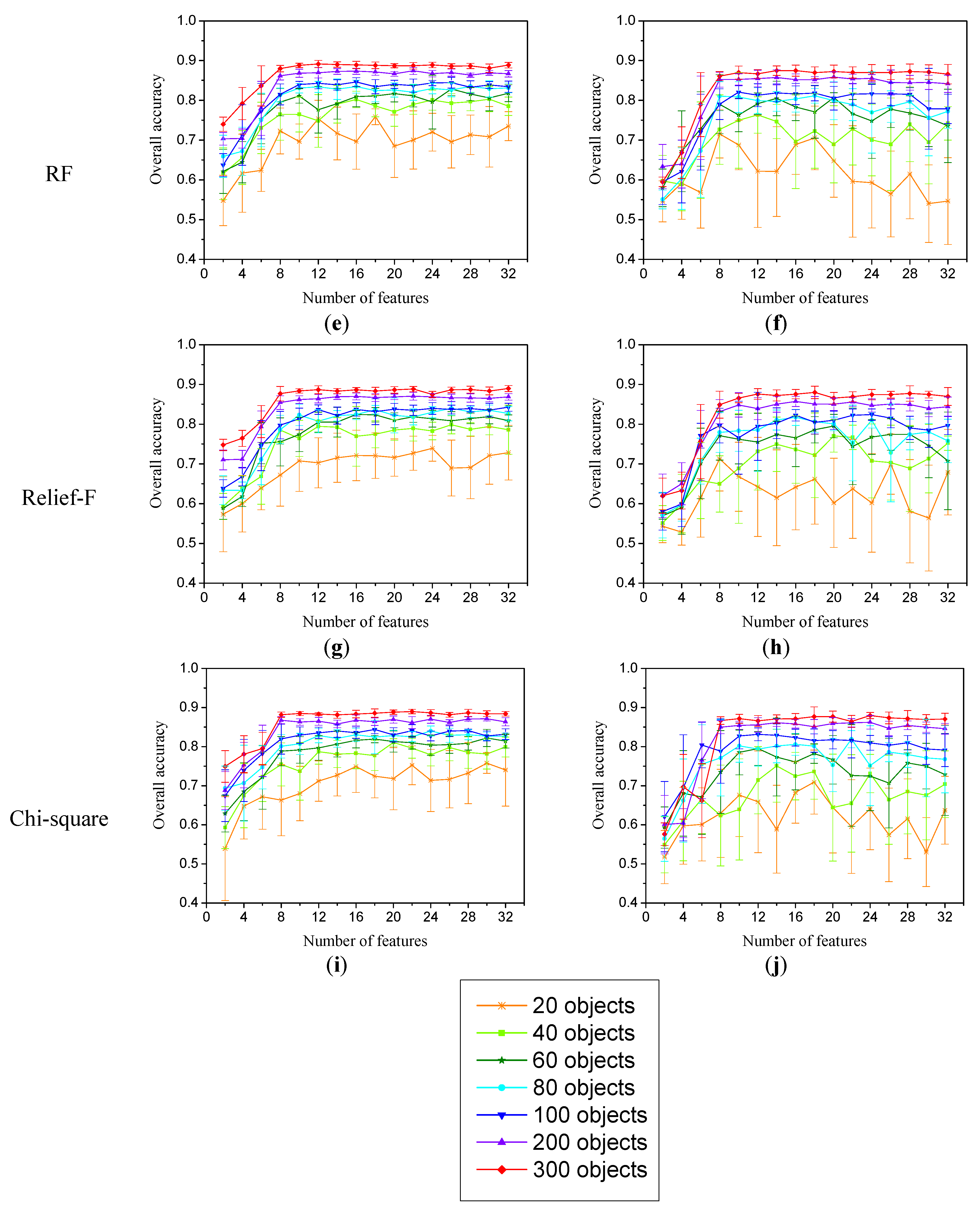
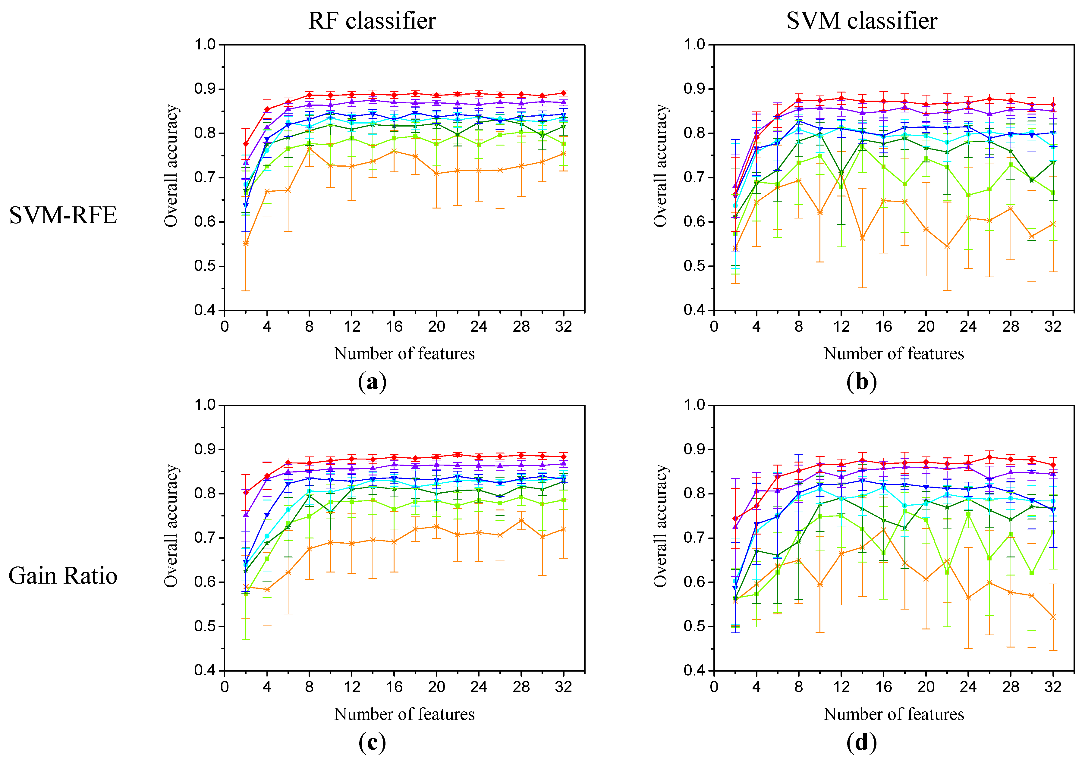
3.1. Evaluation of Feature-Importance-Evaluation Methods

Figure 2 and Figure 3 show the change patterns of the classification accuracy for both classifiers in both areas, as a different number of features was used and the training set size varied. The mean overall accuracy of ten classification iterations with a fixed number of features and the same training set size was calculated for the different feature-importance-evaluation methods. The mean overall accuracy initially tended to increase rapidly with an increasing number of features used. After a certain threshold was reached, the classification accuracy remained stable, even if more features were added. Furthermore, a slightly different classification performance was observed between both classifiers for varying training set sizes, even the use of different feature selection methods. For area 1, when the training set size was less than 60 objects, the classification accuracy of the SVM classifier rose to a peak with the additional features and thereafter declined when adding more features (Figure 2), which is in line with earlier findings for hyperspectral data studies [5]. A similar pattern was also observed in area 2 (Figure 3). However, for both areas, the RF classifier overall outperformed the SVM classifier, and the classification accuracy was relatively stable with the variation of features when small training set sizes were used. Therefore, it was further evident that the RF classifier is less sensitive to the effect of data dimensionality compared to the SVM classifier, even though a small training set size was used, and Li et al. [19] proved that either classifier could be used with limited training samples. It should also be noted that our results do not agree with the early findings that SVM is insensitive to the Hughes effect, but are in line with Pal and Foody [5], who determined that SVM classification is influenced by the number of features used. We assumed that additional features could compensate for the lack of training samples for the RF classifier and that SVM is prone to the Hughes effect for object-based classification with the lack of training samples regardless of the use of additional features.
We can note that the results varied dramatically between several training set sizes, but slightly different performances were still observed between feature selection algorithms with respect to the limitations of features. For example, the performance when using a small number of features highly depends on the feature-importance-evaluation methods, while different feature selection methods likely imply a different ranked list of features, even when the same training set size is used [37]. A two-tailed t-test was used to compare the difference of the statistical significance between the means of the respective accuracies generated using all features and those derived from the ranked list of the features (Table 2) to obtain a sound conclusion. Table 2 shows the results of the statistical significance tests achieved using a training set size of 300 objects for area 1, which is likely insensitive to the Hughes effect (the dimensionality of the data) according to the previous analysis. The results highlight that the efficiency of the feature selection methods was different when a small number of features was used, because the comparable accuracy with a full feature set was achieved by requiring a different number of features, and also different performance was observed in a small number of features for each algorithm even using the same classifier. For both classifiers, Gain Ratio and SVM-RFE were better than the other feature-importance-evaluation methods because of the lower statistical values obtained when using a small number of features (Table 2). However, regarding the efficiency of feature selection for the RF classifier, it was evident that SVM-RFE and Chi-square are both appropriate feature selection methods. The differences leveled out when a smaller number of features (8 features) was used compared to the other three algorithms (Table 2). For the SVM classifier, all five feature-importance-evaluation methods achieved a comparable accuracy with the full feature set when eight features were used (Table 2). These results are similar to those of Ghosh & Joshi [49], who proved that the accuracy could saturate and show no change after the inclusion of the first ten variables when using RFE technique with transformation variables (e.g., principal component). Therefore, it seems that the SVM-RFE method may be suitable for the RF classifier, while Gain Ratio and SVM-RFE are both suitable for the SVM classifier.

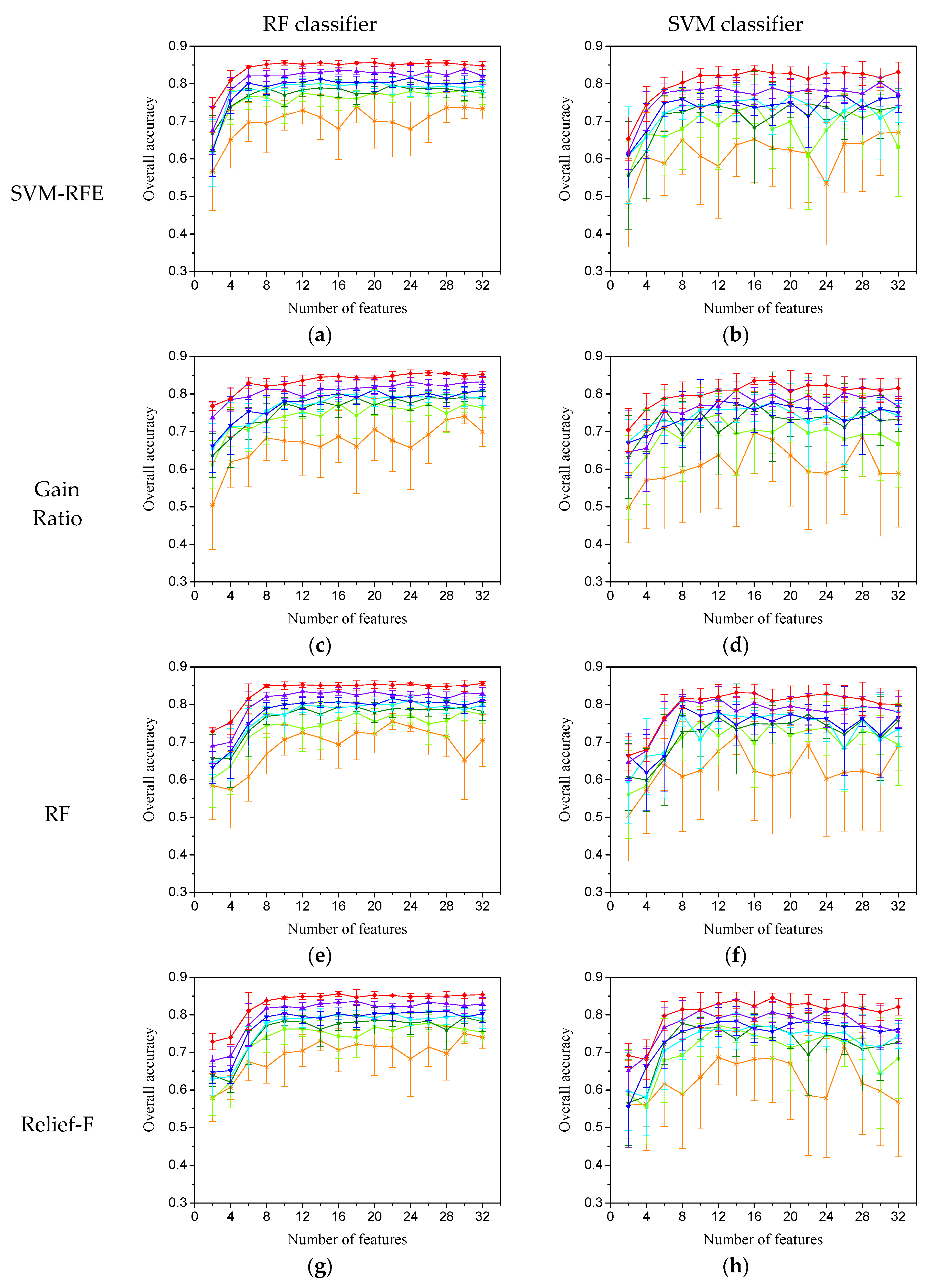
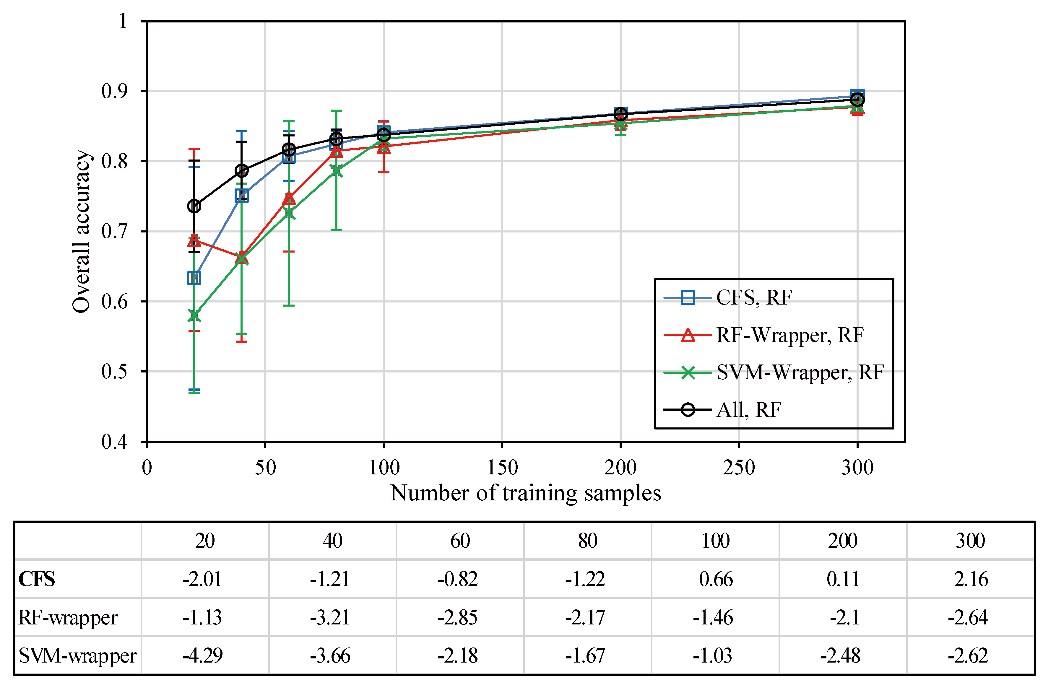
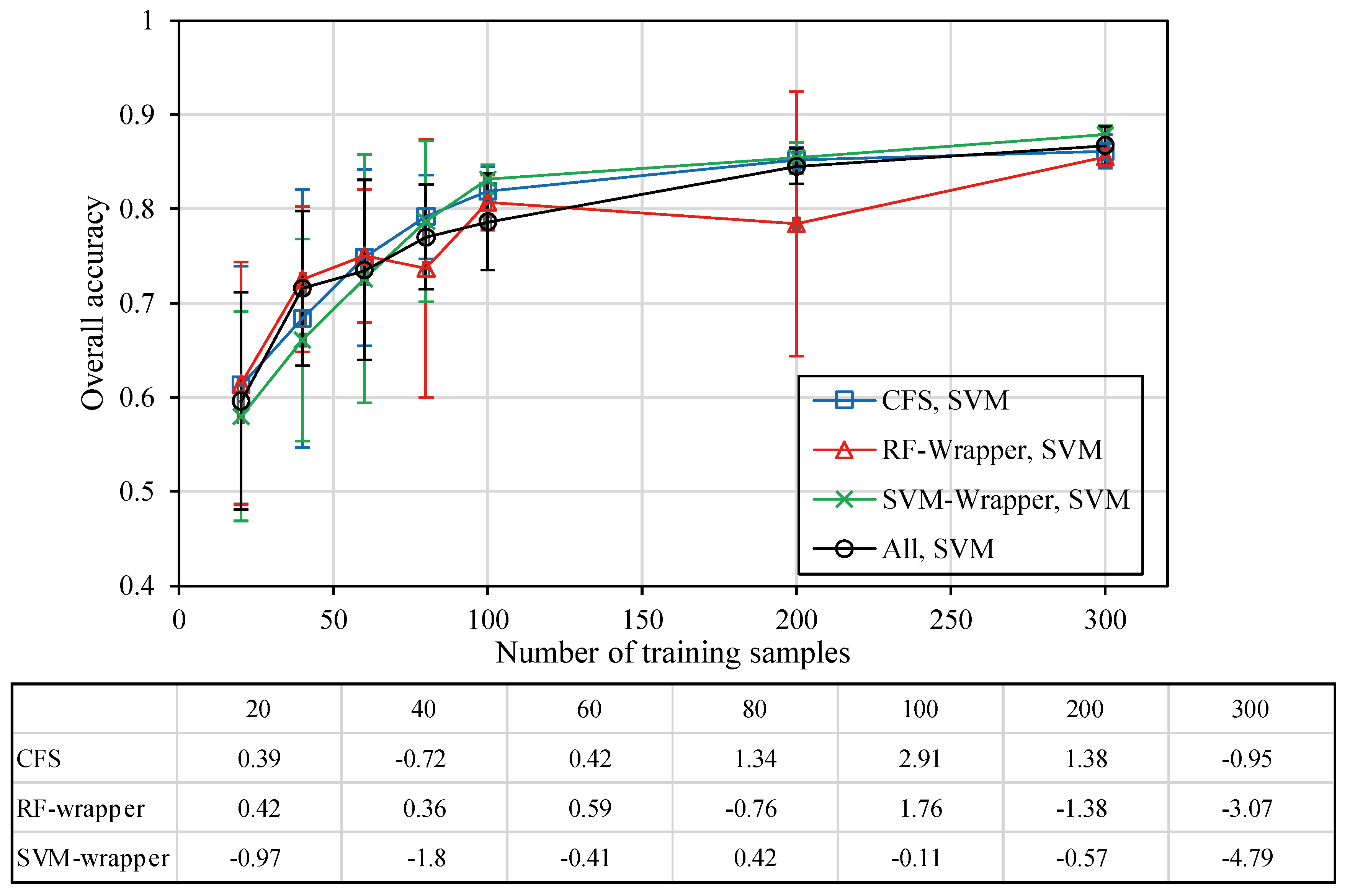
3.2. Evaluation for Feature-Subset-Evaluation Methods

The mean overall accuracy curves and the standard errors for three feature-subset-evaluation methods are reported in Figure 4 and Figure 5. Irrespective of the strategies of combination between feature selection methods and classification algorithms employed, these results are in line with the established fact that the mean accuracy increases and the standard error declines along with an increasing training set size [9]. Furthermore, the statistically significant difference between the overall accuracies derived from the three feature-subset-evaluation methods and that generated using all features was assessed using a two-tailed t-test method. For the RF classifier, the results highlighted that the classification performance using the selected features of CFS was in most cases significantly similar to that derived using all features, while the statistically significant negative impact of feature selection was frequently observed for both wrapper methods (Figure 4). It could be attributed to the sensitivity of the RF to limited training samples, as the method greatly benefits from a larger sample size [50]. For the SVM classifier, the results yielded that there was generally no statistically significant difference in the overall accuracy between using features selected with the three feature-subset-evaluation methods and the full feature set (Figure 5), especially for a small training set size, since the composition of support vectors could not be changed significantly by adding more training instances to span the separating hyperplane [51]. Thus, the SVM classifier seems to benefit from the three feature-subset-evaluation methods even though no statistically significant accuracy improvement occurred, because the reduced features were nonetheless able to improve the efficiency of the classification process.

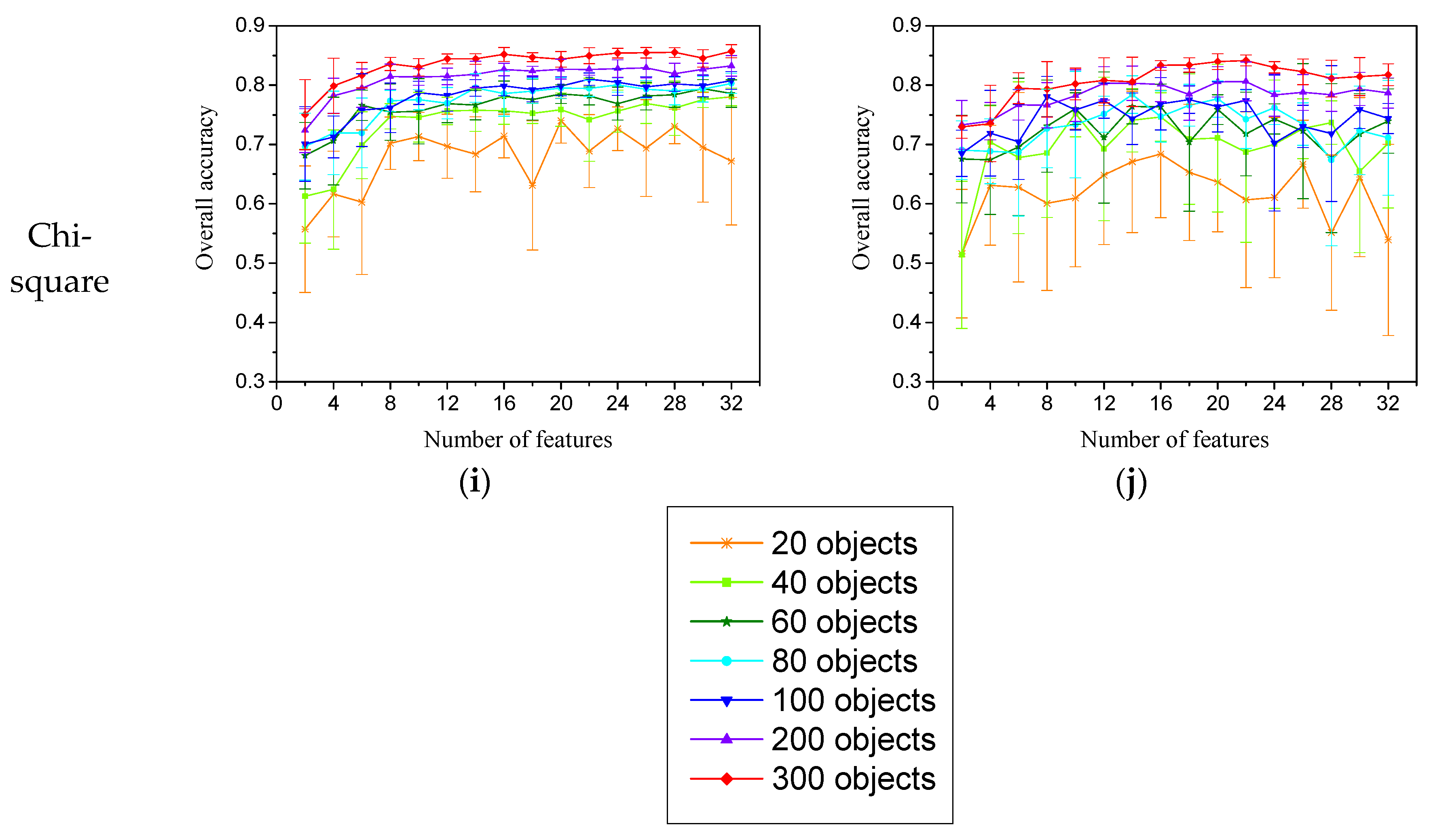
3.3. Comprehensive Evaluation for All Feature Selection Methods

In order to assess all feature selection methods considered in this study, the statistically significant difference between the best accuracy obtained using the selected features and that derived from the full feature set was evaluated using a two-tailed t-test, as well as an assessment of the responses of all considered feature selection methods and both classifiers versus the parameter of the training set size (Table 3). In terms of the three feature-subset-evaluation approaches, only one optimal feature subset could be derived for single sampling, while a series of feature subsets were likely to be derived from the ranked feature list for the feature-importance-evaluation methods, and we therefore considered that the best classification accuracy was obtained from this optimal feature subset for the feature-subset-evaluation approaches. In Table 3, decimal numbers may occur in brackets for these three feature-subset-evaluation approaches, because the number of features is here represented by the mean number of the selected features based on the ten classification repetitions. The number of optimal features was not necessarily consistent for each classification repetition, due to the changing training samples.
Regarding the comparison between the two types of results of feature selection, features acquired from feature-importance-evaluation always had a positive effect on the performance of the object-based classification, whichever classifiers were used, while a negative impact was frequently observed for a feature subset derived from the two wrapper methods. It seems that the wrapper methods do not retain the superiority for object-based classification, which is claimed in per-pixel hyperspectral data [37,52,53]. Additionally, the three feature-subset-evaluation methods tended to use small numbers of features as the optimal feature subset, in particular for both wrapper methods, while the other feature-importance-evaluation methods proved that relatively large numbers of features were likely to achieve the best classification accuracy (Table 3). We assume that this is related to the overestimation of the performance of the classifier, due to the point-based cross-validation in the process of the wrapper method [54,55], so that the best accuracy was mostly achieved for smaller numbers of features, especially when the learning scheme of the wrapper method was an RF classifier. Following Johnson [56], we also presented this issue using a point-based accuracy assessment method for cross-validation of wrapper-based feature selection within an object-based classification, since the segmented object is not necessarily represented as only one class because of the possible occurrence of mixed objects [9]. In a future study, we recommend a polygon-based accuracy assessment method to be used for cross-validation in the process of wrapper-based feature selection.
On the other hand, the best classification accuracy was generated from the ranked features. This was significantly better than that derived from the full feature set and demonstrates that feature selection carries the potential of improving the object-based classification, even though the classification accuracies using feature-subset-evaluation methods have no superiority to those derived using all features, due to the limited features determined. Thus, it seems that feature-importance-evaluation methods are more appropriate for object-based classification, and the wrapper methods are necessary to employ a polygon-based cross-validation.
For feature-importance-evaluation methods, the RF classifier benefited significantly from RF and SVM-RFE feature selection methods, whereas no significant improvement was observed for both other methods (Gain ratio and Relief-F) (Table 3). Contrarily, the SVM classifier can obtain the most significant improvement from all five evaluated feature-importance-evaluation methods. Moreover, if the goal is to optimize the accuracy of object-based classification, we may suggest using feature-importance-evaluation methods, while feature-subset-evaluation methods did not significantly improve the classification accuracy in any case. In addition, our experiment (using a maximum of 32) revealed that the optimal number of input features for obtaining the best classification is between 15–25 features for the RF classifier. However, in most cases that used the feature-importance-evaluation methods in combination with the SVM classifier, the results revealed that relatively small feature sets (10–20) achieved the best accuracy.

4. Conclusions

In this study, several advanced feature selection methods were assessed for an object-based classification of agricultural areas using UAV imagery and RF and SVM classifiers. A major conclusion is that the RF classifier is relatively insensitive to the dimensionality of the data, and the SVM classifier benefits more from a feature selection analysis regarding accuracy, especially for small training set sizes. Moreover, SVM is easily affected by the number of input features, namely the Hughes phenomenon, when small training samples are used.
The results also highlight that it is crucial to select an appropriate feature selection method since the performance varied greatly in most cases. For example, with feature-importance-evaluation methods, a comparable accuracy was initially obtained using different numbers of features, while the various classification accuracies were achieved with the same number of features (Table 1). For the RF classification using both wrapper methods, a statistically significant reduction in accuracy was observed, mostly independent of training set size (Figure 4). Thus, CFS may be an appropriate feature-subset-evaluation method, as a reduced data set can yield a similar classification accuracy compared to that derived from the full feature set. Finally, the results of feature-importance-evaluation methods demonstrate that object-based classification can benefit from undertaking a feature selection analysis before classification, but one may anticipate that a polygon-based cross-validation could be even more suitable to further improve the feature selection for object-based classification for the wrapper method.
For the classification procedure using feature-importance-evaluation methods, 15–25 input features are likely to produce the best classification results for the RF classifier in most cases. For the SVM classifier, 10–20 input features generally produce the best results, depending on the feature selection algorithm and the training set size. The idea about the wrapper method has not been proven in previous studies, and the authors therefore hope that these findings support the further advancement and maturation of OBIA classification methodologies. In future work, we therefore expect that wrapper methods with polygon-based cross-validation may further improve the performance of wrapper methods on object-based classification.

Acknowledgments

This work is supported by a Project funded by China Postdoctoral Science Foundation (No. 2016M600392), the Program B for Outstanding PhD Candidate of Nanjing University (No. 201502B008), the Special Research Fund of the Ministry of Land and Resources for NonProfit Sector (No. 201411014-03), and the National Natural Science Foundation of China (No. 41601497). Sincere thanks are given for the comments and contributions of anonymous reviewers and members of the editorial team.

Author Contributions

Lei Ma and Manchun Li conceived and designed the experiments; Lei Ma performed the experiments, results interpretation, and manuscript writing; Thomas Blaschke and Dirk Tiede assisted with refining the research design and manuscript writing, and also helped improving the English; Tengyu Fu and Zhenjin Zhou revised the manuscript, and contributed images/materials/analysis tools; Xiaoxue Ma and Deliang Chen assisted with the experimental result analysis, and helped checking the whole text and data.

Conflicts of Interest

The authors declare no conflicts of interest.

References

  1. Pedergnana, M.; Marpu, P.R.; Dalla Mura, M.; Benediktsson, J.A.; Bruzzone, L. A novel technique for optimal feature selection in attribute profiles based on genetic algorithms. IEEE Trans. Geosci. Remote Sens. 2013, 51, 3514–3528. [Google Scholar] [CrossRef]
  2. Novack, T.; Esch, T.; Kux, H.; Stilla, U. Machine learning comparison between worldview-2 and quickbird-2-simulated imagery regarding object-based urban land cover classification. Remote Sens. 2011, 3, 2263–2282. [Google Scholar] [CrossRef]
  3. Topouzelis, K.; Psyllos, A. Oil spill feature selection and classification using decision tree forest on SAR image data. ISPRS J. Photogramm. Remote Sens. 2012, 68, 135–143. [Google Scholar] [CrossRef]
  4. Melgani, F.; Bruzzone, L. Classification of hyperspectral remote sensing images with support vector machines. IEEE Trans. Geosci. Remote Sens. 2004, 42, 1778–1790. [Google Scholar] [CrossRef]
  5. Pal, M.; Foody, G.M. Feature selection for classification of hyperspectral data by SVM. IEEE Trans. Geosci. Remote Sens. 2010, 48, 2297–2307. [Google Scholar] [CrossRef]
  6. Cheng, G.; Han, J. A survey on object detection in optical remote sensing images. ISPRS J. Photogramm. Remote Sens. 2016, 117, 11–28. [Google Scholar] [CrossRef]
  7. Laliberte, A.S.; Browning, D.; Rango, A. A comparison of three feature selection methods for object-based classification of sub-decimeter resolution ultracam-l imagery. Int. J. Appl. Earth Obs. Geoinf. 2012, 15, 70–78. [Google Scholar] [CrossRef]
  8. Blaschke, T.; Hay, G.J.; Kelly, M.; Lang, S.; Hofmann, P.; Addink, E.; Feitosa, R.Q.; Meer, F.V.D.; Werff, H.V.D.; Coillie, F.V. Geographic object-based image analysis—Towards a new paradigm. ISPRS J. Photogramm. Remote Sens. 2014, 87, 180–191. [Google Scholar] [CrossRef] [PubMed]
  9. Ma, L.; Cheng, L.; Li, M.; Liu, Y.; Ma, X. Training set size, scale, and features in geographic object-based image analysis of very high resolution unmanned aerial vehicle imagery. ISPRS J. Photogramm. Remote Sens. 2015, 102, 14–27. [Google Scholar] [CrossRef]
  10. Duro, D.C.; Franklin, S.E.; Dubé, M.G. Multi-scale object-based image analysis and feature selection of multi-sensor earth observation imagery using random forests. Int. J. Remote Sens. 2012, 33, 4502–4526. [Google Scholar] [CrossRef]
  11. Stumpf, A.; Kerle, N. Object-oriented mapping of landslides using random forests. Remote Sens. Environ. 2011, 115, 2564–2577. [Google Scholar] [CrossRef]
  12. Puissant, A.; Rougier, S.; Stumpf, A. Object-oriented mapping of urban trees using random forest classifiers. Int. J. Appl. Earth Obs. Geoinf. 2014, 26, 235–245. [Google Scholar] [CrossRef]
  13. Han, J.; Pei, J.; Kamber, M. Data Mining: Concepts and Techniques; Elsevier: Amsterdam, The Netherlands, 2011. [Google Scholar]
  14. Chubey, M.S.; Franklin, S.E.; Wulder, M.A. Object-based analysis of Ikonos-2 imagery for extraction of forest inventory parameters. Photogramm. Eng. Remote Sens. 2006, 72, 383–394. [Google Scholar] [CrossRef]
  15. Laliberte, A.S.; Rango, A. Texture and scale in object-based analysis of subdecimeter resolution unmanned aerial vehicle (UAV) imagery. IEEE Trans. Geosci. Remote Sens. 2009, 47, 761–770. [Google Scholar] [CrossRef]
  16. Vieira, M.A.; Formaggio, A.R.; Rennó, C.D.; Atzberger, C.; Aguiar, D.A.; Mello, M.P. Object based image analysis and data mining applied to a remotely sensed landsat time-series to map sugarcane over large areas. Remote Sens. Environ. 2012, 123, 553–562. [Google Scholar] [CrossRef]
  17. Peña-Barragán, J.M.; Ngugi, M.K.; Plant, R.E.; Six, J. Object-based crop identification using multiple vegetation indices, textural features and crop phenology. Remote Sens. Environ. 2011, 115, 1301–1316. [Google Scholar] [CrossRef]
  18. Yu, Q.; Gong, P.; Clinton, N.; Biging, G.; Kelly, M.; Schirokauer, D. Object-based detailed vegetation classification with airborne high spatial resolution remote sensing imagery. Photogramm. Eng. Remote Sens. 2006, 72, 799–811. [Google Scholar] [CrossRef]
  19. Li, M.; Ma, L.; Blaschke, T.; Cheng, L.; Tiede, D. A systematic comparison of different object-based classification techniques using high spatial resolution imagery in agricultural environments. Int. J. Appl. Earth Obs. Geoinf. 2016, 49, 87–98. [Google Scholar] [CrossRef]
  20. Pal, M.; Mather, P. Some issues in the classification of dais hyperspectral data. Int. J. Remote Sens. 2006, 27, 2895–2916. [Google Scholar] [CrossRef]
  21. Van Coillie, F.M.; Verbeke, L.P.; De Wulf, R.R. Feature selection by genetic algorithms in object-based classification of IKONOS imagery for forest mapping in flanders, Belgium. Remote Sens. Environ. 2007, 110, 476–487. [Google Scholar] [CrossRef]
  22. Weston, J.; Mukherjee, S.; Chapelle, O.; Pontil, M.; Poggio, T.; Vapnik, V. Feature selection for SVMS. Adv. Neural Inf. Process. Syst. 2000, 13, 668–674. [Google Scholar]
  23. Guyon, I.; Weston, J.; Barnhill, S.; Vapnik, V. Gene selection for cancer classification using support vector machines. Mach. Learn. 2002, 46, 389–422. [Google Scholar] [CrossRef]
  24. Duro, D.C.; Franklin, S.E.; Dubé, M.G. A comparison of pixel-based and object-based image analysis with selected machine learning algorithms for the classification of agricultural landscapes using SPOT-5 HRG imagery. Remote Sens. Environ. 2012, 118, 259–272. [Google Scholar] [CrossRef]
  25. Ma, L.; Cheng, L.; Han, W.; Zhong, L.; Li, M. Cultivated land information extraction from high-resolution unmanned aerial vehicle imagery data. J. Appl. Remote Sens. 2014, 8, 1–25. [Google Scholar] [CrossRef]
  26. Peña, J.M.; Torres-Sánchez, J.; de Castro, A.I.; Kelly, M.; López-Granados, F. Weed mapping in early-season maize fields using object-based analysis of unmanned aerial vehicle (UAV) images. PLoS ONE 2013, 8, e77151. [Google Scholar]
  27. Ma, L.; Wang, Y.; Li, M.; Tong, L.; Cheng, L. Using high-resolution imagery acquired with an autonomous unmanned aerial vehicle for urban construction and planning. In Proceedings of the International Conference on Remote Sensing, Environment and Transportation Engineering, Najing, China, 26–28 July 2013.
  28. Baatz, M.; Schäpe, A. Multiresolution segmentation: An optimization approach for high quality multi-scale image segmentation. In Angewandte Geographische Informationsverarbeitung XII; Strobl, J., Blaschke, T., Griesebner, G., Eds.; Herbert Wichmann Verlag: Berlin, Germany, 2000; Volume 58, pp. 12–23. [Google Scholar]
  29. Hall, M.; Frank, E.; Holmes, G.; Pfahringer, B.; Reutemann, P.; Witten, I.H. The weka data mining software: An update. ACM SIGKDD Explor. Newsl. 2009, 11, 10–18. [Google Scholar] [CrossRef]
  30. Zhao, Z.; Morstatter, F.; Sharma, S.; Alelyani, S.; Anand, A.; Liu, H. Advancing Feature Selection Research: Asu Feature Selection Repository; TR-10-007; School of Computing, Informatics, and Decision Systems Engineering, Arizona State University: Tempe, AZ, USA, 2007. [Google Scholar]
  31. Liu, H.; Setiono, R. Chi2: Feature selection and discretization of numeric attributes. In Proceedings of the Seventh IEEE International Conference on Tools with Artificial Intelligence, Herndon, VA, USA, 29–31 May 1995; pp. 388–391.
  32. Gilad-Bachrach, R.; Navot, A.; Tishby, N. Margin based feature selection-theory and algorithms. In Proceedings of the Twenty-First International Conference on Machine Learning, Banff, AB, Canada, 4–8 July 2004; ACM: New York, NY, USA; p. 43.
  33. Robnik-Šikonja, M.; Kononenko, I. Theoretical and empirical analysis of relieff and rrelieff. Mach. Learn. 2003, 53, 23–69. [Google Scholar] [CrossRef]
  34. Verikas, A.; Gelzinis, A.; Bacauskiene, M. Mining data with random forests: A survey and results of new tests. Pattern Recogn. 2011, 44, 330–349. [Google Scholar] [CrossRef]
  35. Hall, M.A.; Holmes, G. Benchmarking attribute selection techniques for discrete class data mining. IEEE Trans. Knowl. Data Eng. 2003, 15, 1437–1447. [Google Scholar] [CrossRef]
  36. Phuong, T.M.; Lin, Z.; Altman, R.B. Choosing SNPS using feature selection. J. Bioinf. Comput. Biol. 2006, 4, 241–257. [Google Scholar] [CrossRef]
  37. Kohavi, R.; John, G.H. Wrappers for feature subset selection. Artif. Intell. 1997, 97, 273–324. [Google Scholar] [CrossRef]
  38. Maldonado, S.; Weber, R. A wrapper method for feature selection using support vector machines. Inf. Sci. 2009, 179, 2208–2217. [Google Scholar] [CrossRef]
  39. Rodin, A.S.; Litvinenko, A.; Klos, K.; Morrison, A.C.; Woodage, T.; Coresh, J.; Boerwinkle, E. Use of wrapper algorithms coupled with a random forests classifier for variable selection in large-scale genomic association studies. J. Comput. Biol. 2009, 16, 1705–1718. [Google Scholar] [CrossRef] [PubMed]
  40. Platt, J.C. 12 fast training of support vector machines using sequential minimal optimization. In Advances in Kernel Methods: Support Vector Learning; MIT Press: Cambridge, MA, USA, 1999; pp. 185–208. [Google Scholar]
  41. Whiteside, T.G.; Maier, S.W.; Boggs, G.S. Area-based and location-based validation of classified image objects. Int. J. Appl. Earth Obs. Geoinf. 2014, 28, 117–130. [Google Scholar] [CrossRef]
  42. Stefanski, J.; Mack, B.; Waske, B. Optimization of object-based image analysis with random forests for land cover mapping. IEEE J. Sel. Topics Appl. Earth Observ. Remote Sens. 2013, 6, 2492–2504. [Google Scholar] [CrossRef]
  43. Pal, M. Random forest classifier for remote sensing classification. Int. J. Remote Sens. 2005, 26, 217–222. [Google Scholar] [CrossRef]
  44. Rodriguez-Galiano, V.F.; Ghimire, B.; Rogan, J.; Chica-Olmo, M.; Rigol-Sanchez, J.P. An assessment of the effectiveness of a random forest classifier for land-cover classification. ISPRS J. Photogramm. Remote Sens. 2012, 67, 93–104. [Google Scholar] [CrossRef]
  45. Cheng, G.; Han, J.; Zhou, P.; Guo, L. Multi-class geospatial object detection and geographic image classification based on collection of part detectors. ISPRS J. Photogramm. Remote Sens. 2014, 98, 119–132. [Google Scholar] [CrossRef]
  46. Mountrakis, G.; Im, J.; Ogole, C. Support vector machines in remote sensing: A review. ISPRS J. Photogramm. Remote Sens. 2011, 66, 247–259. [Google Scholar] [CrossRef]
  47. Chang, C.-C.; Lin, C.-J. LIBSVM: A library for support vector machines. ACM Trans. Intell. Syst. Technol. (TIST) 2011, 2, 27. [Google Scholar] [CrossRef]
  48. Shao, Y.; Lunetta, R.S. Comparison of support vector machine, neural network, and cart algorithms for the land-cover classification using limited training data points. ISPRS J. Photogramm. Remote Sens. 2012, 70, 78–87. [Google Scholar] [CrossRef]
  49. Ghosh, A.; Joshi, P. A comparison of selected classification algorithms for mapping bamboo patches in lower gangetic plains using very high resolution worldview 2 imagery. Int. J. Appl. Earth Obs. Geoinf. 2014, 26, 298–311. [Google Scholar] [CrossRef]
  50. Fassnacht, F.; Hartig, F.; Latifi, H.; Berger, C.; Hernández, J.; Corvalán, P.; Koch, B. Importance of sample size, data type and prediction method for remote sensing-based estimations of aboveground forest biomass. Remote Sens. Environ. 2014, 154, 102–114. [Google Scholar] [CrossRef]
  51. Wieland, M.; Pittore, M. Performance evaluation of machine learning algorithms for urban pattern recognition from multi-spectral satellite images. Remote Sens. 2014, 6, 2912–2939. [Google Scholar] [CrossRef]
  52. Chan, J.C.-W.; Paelinckx, D. Evaluation of random forest and adaboost tree-based ensemble classification and spectral band selection for ecotope mapping using airborne hyperspectral imagery. Remote Sens. Environ. 2008, 112, 2999–3011. [Google Scholar] [CrossRef]
  53. Huang, X.; Zhang, L. An svm ensemble approach combining spectral, structural, and semantic features for the classification of high-resolution remotely sensed imagery. IEEE Trans. Geosci. Remote Sens. 2013, 51, 257–272. [Google Scholar] [CrossRef]
  54. Cheng, G.; Han, J.; Guo, L.; Liu, Z.; Bu, S.; Ren, J. Effective and efficient midlevel visual elements-oriented land-use classification using VHR remote sensing images. IEEE Trans. Geosci. Remote Sens. 2015, 53, 4238–4249. [Google Scholar] [CrossRef]
  55. Sun, L.; Schulz, K. Response to johnson ba scale issues related to the accuracy assessment of land use/land cover maps produced using multi-resolution data: Comments on “the improvement of land cover classification by thermal remote sensing”. Remote Sens. 2015, 7, 13440–13447. [Google Scholar] [CrossRef]
  56. Johnson, B.A. Scale issues related to the accuracy assessment of land use/land cover maps produced using multi-resolution data: Comments on “the improvement of land cover classification by thermal remote sensing”. Remote Sens. 2015, 7, 13436–13439. [Google Scholar] [CrossRef]
Figure 1. Study area in the southwest of China showing the plot acquired by the UAV images. (a) Digital ortho image of area 1 overlaying a segmentation layer at a scale of 100; and (b) the reference layer. (c) Digital ortho image of area 2 overlaying a segmentation layer at a scale of 100; and (d) the reference layer.
Ijgi 06 00051 g001
Figure 2. For area 1, the relationship between the mean overall accuracy of classifications repeated ten times (fixed numbers of features and training set size) and the number of features using five feature-importance-evaluation methods with different training set sizes for both classifiers.
Ijgi 06 00051 g002aIjgi 06 00051 g002b
Figure 3. For area 2, the relationship between the mean overall accuracy of classifications repeated ten times (fixed numbers of features and training set size) and the number of features using five feature-importance-evaluation methods with different training set sizes for both classifiers.
Ijgi 06 00051 g003aIjgi 06 00051 g003b
Figure 4. The overall accuracy versus the training set size obtained by the different feature subset using the RF classifier. The statistical value derived from a two-tailed t-test reveals whether there is a significant difference in the classification accuracy between the selected feature subset and the full set of features.
Ijgi 06 00051 g004
Figure 5. The overall accuracy versus the training set size obtained by the different feature subsets using the SVM classifier and the statistical value derived from a two-tailed t-test reveals whether there is a significant difference in the classification accuracy between the selected feature subset and the full feature set.
Ijgi 06 00051 g005
Table 1. List of object features.
Feature TypeFeature NamesDescription
SpectralMean blue, mean green, mean red, max difference, standard deviation (std. dev.) blue, std. dev. green, std. dev. red, brightness Spectral features were used to evaluate the first (mean), second (standard deviation) of an image object’s pixel value.
TextureGLCM (Gray-Level Co-occurrence Matrix) homogeneity, GLCM contrast, GLCM dissimilarity, GLCM entropy, GLCM std. dev., GLCM correlation, GLCM ang. 2nd moment, GLCM mean, GLDV (Gray-Level Difference Vector) ang. 2nd moment, GLDV entropy, GLDV mean, GLDV contrast Texture features are derived from texture after Haralick based on the Gray-Level Co-occurrence Matrix or Gray-Level Difference Vector.
ShapeArea, compactness, density, roundness, main direction, rectangular fit, elliptic fit, asymmetry, border index, shape index Shape features refer to the geometry information of meaningful objects, which is calculated from the pixels that form it. An accurate segmentation of the map is necessary to ensure the use of these features successfully.
Table 2. Summary of the test for the differences between the classifications with feature subsets following an ascending order and that derived from the full feature set. The statistical value was derived from a two-tailed t-test. The difference is significant at the 0.05 significance level if the absolute value of the test statistics is greater than 1.96. The positive number indicates that the mean accuracy of the full feature set was better than that derived from the selected subset, otherwise the subset was better.
Number of FeaturesGain RatioRelief-FRFSVM-RFEChi-Square
RFSVMRFSVMRFSVMRFSVMRFSVM
25.815.1526.3215.1123.3529.829.687.149.8727.13
44.094.1317.5113.827.058.544.953.726.536.17
62.822.56.053.543.062.725.262.526.336.52
82.491.471.981.532.390.551.37−1.350.820.64
102.01−0.131.940.480.15−0.381.35−1.34−0.23−0.15
121.04−0.060.76−0.69−0.74−0.081.05−1.940.340.7
141.14−1.271.96−0.29−0.46−0.980.67−0.980.8−0.02
160.32−0.461.06−0.67−0.11−0.941.24−0.810.23−0.08
180.86−0.511.54−1.10.16−0.390.32−0.71−0.35−0.65
200.03−0.990.870.50.52−0.71.85−0.02−1.5−0.91
22−1.33−0.360.40.090.41−0.460.99−0.27−2.070.85
24−0.03−0.574.09−0.53−0.19−0.360.42−0.57−0.72−1.58
26−0.15−2.311.02−0.550.84−0.421.2−1.890.92−0.43
28−0.76−1.830.73−0.740.6−0.660.85−1.16−0.62−0.13
30−0.32−1.751.47−0.591.82−0.522.220.020.030.18
Table 3. Summary of the differences between the best accuracy for the selected feature subsets and that derived using all features. The statistical value was derived from a two-tailed t-test, and the difference is significant at the 0.05 significance level if the absolute value of the test statistic is greater than 1.96. The positive number indicates that the best mean accuracy for the feature subsets was better than that derived using all features, otherwise the latter was better than the former. The values in brackets are the number of features used for the best classification accuracy.
20 Objects40 Objects60 Objects100 Objects200 Objects300 Objects
RFSVMRFSVMRFSVMRFSVMRFSVMRFSVM
Gain Ratio0.35(28)4.2(16)0.69(28)2.4(18)0.0084(28)3.1(12)0.46(22)4.2(14)−0.52(16)2.2(18)0.63(22)2.7(26)
Relief-F0.26(24)3.7(8)1.2(26)3.1(20)1.8(16)3.6(20)0.49(24)4.4(24)0.89(22)2.4(16)0.35(22)2.1(18)
RF2.02(18)4.6(8)1.4(30)2.5(12)1.9(26)5.1(20)2.3(16)3.8(10)2.1(22)2.6(20)1.2(12)1.5(14)
SVM-RFE1.83(8)4.8(12)1.6(28)2.4(14)3.3(26)4(10)2.2(10)3.4(8)2.7(14)3(18)1.1(18)2.2(12)
Chi-square1.74(30)3.6(18)3.7(20)1.1(14)0.69(30)3.1(12)1.7(18)5(12)1.8(30)2.6(24)1.1(22)3.1(24)
CFS−2.01(2.9)0.39(3)−1.21(4.6)−0.72(4.6)−0.82(5.4)0.42(5.9)0.66(7.5)2.91(6.3)0.11(8.1)1.38(8.4)2.16(9)−0.95(9.2)
RF wrapper−1.13(3)0.42(2.5)−3.21(3.8)0.36(3.9)−2.85(3.2)0.59(3.5)−1.46(5.4)1.76(4.4)−2.1(5.6)−1.38(5.2)−2.64(6.2)−3.07(5.6)
SVM wrapper−4.29(3)−0.97(2)−3.66(3.8)−1.8(3.7)−2.18(4.1)−0.41(5.1)−1.03(7)−0.11(6)−2.48(6.7)−0.57(6.4)−2.62(6.9)−4.79(6.1)

