Abstract
Existing data models for moving objects in networks are often limited by flexibly controlling the granularity of representing networks and the cost of location updates and do not encompass semantic information, such as traffic states, traffic restrictions and social relationships. In this paper, we aim to fill the gap of traditional network-constrained models and propose a hierarchical graph model called the Geo-Social-Moving model for moving objects in Networks (GSMNet) that adopts four graph structures, RouteGraph, SegmentGraph, ObjectGraph and MoveGraph, to represent the underlying networks, trajectories and semantic information in an integrated manner. The bulk of user-defined data types and corresponding operators is proposed to handle moving objects and answer a new class of queries supporting three kinds of conditions: spatial, temporal and semantic information. Then, we develop a prototype system with the native graph database system Neo4Jto implement the proposed GSMNet model. In the experiment, we conduct the performance evaluation using simulated trajectories generated from the BerlinMOD (Berlin Moving Objects Database) benchmark and compare with the mature MOD system Secondo. The results of 17 benchmark queries demonstrate that our proposed GSMNet model has strong potential to reduce time-consuming table join operations an d shows remarkable advantages with regard to representing semantic information and controlling the cost of location updates.
1. Introduction
Moving Objects Databases (MOD) focus on modeling and querying the movements of moving entities, such as people, vehicles and vessels. With the development of positioning technologies, such as Global Positioning System (GPS) and Radio-Frequency Identification (RFID), it has been extensively studied [1,2,3,4] in recent years due to the wide application, such as online Location-Based Services (LBSs), Location-Based Social Networks (LBSNs), intelligent surveillance systems based on sensor networks [5,6,7,8], video surveillance systems [9,10,11] and vehicular ad hoc networks [12,13]. In the real world, more moving objects, such as pedestrians, cars and buses, are inclined to move along with underlying transportation networks other than geographical free space. Hence, the topic of modeling moving objects in networks has received an increasing amount of attention in the literature [14,15,16,17,18,19].
Although there has been much work on modeling moving objects in networks, such as State-Based Dynamic Transportation Network (SBDTN) [20], MODTN [21], Graph of Cellular Automata (GCA) [22] and Moving Objects in Networks (MONET) [23], the approaches only address the issue of representing networks and trajectories and ignore the semantic information, such as traffic states, traffic restrictions and social relationships between moving objects. In addition, how to balance the granularity of modeling networks and the cost of location updates is still also a challenge in the field of MOD and Geographical Information Systems (GIS) [14,24,25]. That is because fine-grained network-constrained models represent the segment as the basic unit. However, this could lead to more cost of location updates and index maintenance, owing to the fact that frequently changing segments of a moving object motivates massive location update requests and causes index structures to be invalidated. In contrast, coarse-grained network-constrained models represent the route as the basic unit. Although it could help to reduce the cost of location updates, because the traffic state is closely related to segments, it cannot adapt well to some real-world applications that require good real-time performance, especially for vehicle navigation systems and carpool services [26,27].
Additionally, existing network-constrained data models are hard to define as spatial-temporal integrated approaches [2,15], due to the lack of the unified and effective management of trajectories, underlying networks and semantic information. Some brute-force approaches store these types of unstructured datasets into multiple tables. However, many complex queries supporting three kinds of conditions, spatial, temporal and semantic information, must rely on time-consuming table join operations. Hence, this requires the development of a novel spatial-temporal integrated data model for moving objects in networks that has the capability of flexible controls for location updates simultaneously.
In this paper, we propose a hierarchical graph model for moving objects in networks called the Geo-Social-Moving data model for moving objects in Networks (GSMNet), which contains four graph structures: RouteGraph, SegmentGraph, ObjectGraph and MoveGraph. To control the cost of location updates, the underlying network is represented as two separate graph structures, RouteGraph and SegmentGraph, at the different levels of granularity. It is different from traditional modeling approaches that represent a transportation network as a directed graph. Routes and segments are represented as two kinds of graph nodes, and spatial relationships such as and connect these graph nodes. One-to-many relationships from route nodes to segment nodes are created to model the topological relationships. Traffic restrictions are represented as edges between segments or route graph nodes. Furthermore, ObjectGraph represents the social relationships between moving objects; MoveGraph aggregates all of the location points in the current segment as one trajectory unit and represents it as a graph node.
The work reported in this paper is a step toward enhancing integrated spatial-temporal data modeling for moving objects in networks by involving hierarchical graph structures to represent trajectories, networks and semantic information. This is also an attempt to balance the trade-off between the flexible control of the granularity of modeling networks and the cost of location updates.
The contributions of this paper lie in the following aspects:
- A hierarchical GSMNet model for moving objects in networks is proposed that represents moving objects’ trajectories, underlying networks and semantic information, including social relationships and traffic, in an integrated manner. It provides an effective and unified means to handle these unstructured data.
- Based on the GSMNet model, a large set of data types and corresponding operators is provided, and we give the formal definitions of data types together with the operation signatures and semantics. Seventeen benchmark queries from BerlinMOD are rewritten in formal SQL-like notation.
- Extensive experiments with simulated trajectories generated by BerlinMOD are conducted to evaluate the efficiency and performance. The results demonstrate that our proposed GSMNet model has strong potential to reduce time-consuming table join operations and has the capability to represent the semantic information.
The remainder of this paper is organized as follows. Section 2 summarizes related works. Section 3 elaborates on our proposed GSMNet model corresponding to a set of data types. Section 4 provides the formal definition of the operators. Section 5 illustrates the benchmark queries from BerlinMOD. Section 6 conducts the experiments. Finally, Section 7 concludes the paper and recommends future work.
2. Related Work
The principle of early network-constrained data models represented networks as a directed or undirected graph , with a set of nodes V and edges E, where the weight values of the edges denoted the lengths of segments or travel times. The position of moving objects was represented as linear referencing or the common two-dimensional coordinate. Then, the trajectories of objects were modeled as a geometry polyline [28,29,30]. The advantage is that it is easy to implement in a mature relational database, such as Oracle and MySQL. The disadvantage is that it is too simplistic to represent real-world network environments, including overpasses, roadways, turn restrictions at intersections or traffic states. Ding and Guting proposed a State-Based Dynamic Transportation Network (SBDTN) model to represent the traffic state by associating dynamic attributes to edges or vertices [20]. However, it did not involve semantic information, such as social relationships. Speicys et al. proposed a computational data model that adopted a two-dimensional representation and graph representation to represent road networks [31]. Chen et al. modeled the traffic behavior and constraints of networks as a Graph of Cellular Automata (GCA) to predict future trajectories [22].
Another classical network-constrained data model represented road networks as a set of routes and junctions defined as . Guting extended the framework of abstract data types to model moving objects in networks and provided new data types . The routes were defined as , where denotes identification, l denotes the road length, c denotes the geometry polyline, denotes the road types and indicates how route locations are to be embedded into space [14]. Based on the earlier work, Xu and Guting further proposed a generic model that included geographical space, network and indoor environments [32]. Chen et al. proposed a spatial-temporal data model to address the challenge of the representation and computation of time geographic entities and relation in road networks [33]. The innovative idea was to transform network time geographic entities in three-dimensional space to two-dimensional space. The advantage of this approach is to make the best of classical spatial databases, such as Oracle and MySQL. A Parallel-Distributed Network-constrained Moving Objects Database (PD-NMOD) was proposed to manage both transportation networks and trajectories in a distributed manner [34]. However, it did not involve semantic information. To overcome the problem of representing locations and analyzing traffic, Ding et al. proposed a Network-Matched Trajectory-based Moving-Object Database (NMTMOD) mechanism and a traffic flow analysis method using the NMTMOD [35]. Qi and Schneider proposed a two-layered data model called Moving Objects in Networks (MONET). The lower layer represents road networks, and the upper layer represents moving objects [23]. The underlying idea of this research is very similar to our study. However, the proposed GSMNet model in this paper provides more flexibility and supports semantic information.
3. GSMNet Model
In this section, we present the GSMNet model that adopts four graph structures: RouteGraph, SegmentGraph, ObjectGraph and MoveGraph to represent the networks, moving objects, trajectories and semantic information, respectively. Simultaneously, we provide application scenarios and examples to elaborate on the principle of the model and the type systems.
3.1. Preliminaries
First, we provide a set of basic types that can be used for the definitions in the following sections.
(1) Basic Types
There are three basic types for the following definitions:
(2) Temporal Types
Two time types are provided to represent the time:
(3) Geometry Types
The geometry types are employed from OGC, which releases a series of specifications about the geometry object model. The proposed GSMNet involves three basic geometry types:
represents a single location in coordinate space and denotes the zero-dimensional geometric object. It has a latitude value and a longitude value. The location of a moving object could be defined as a point.
is a curve with linear interpolation between . For example, the trajectory segment or road segment could be defined as an instance of .
denotes a planar surface and is topologically closed. The boundary of a consists of a set of that make up its exterior and interior boundaries.
3.2. Modeling Networks
Let us assume an application scenario in the real word, as shown in Figure 1. The network contains three routes (gray lines) , , , three junctions (gray circle) , , and 16 segments (black lines) , , …, . Additionally, there are three trajectories , , .
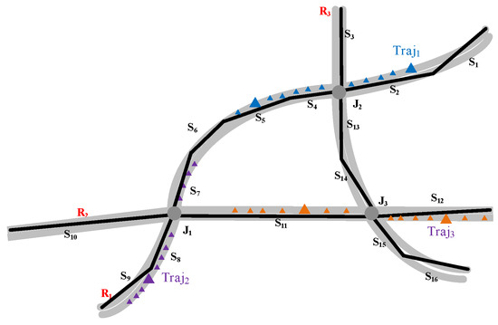
Figure 1.
Road networks.
3.3. Moving Object Representation
(4) Segment
A segment is the specific representation of a portion of a network with the following characteristics: crossing roads are separated by an intersection, and bisecting road segments do not share an intersection. Simultaneously, a segment represents the basic unit of separating traffic flow and is defined as follows:
where is the identifier of segment , g describes the geometry, l denotes the length, is used to denote two types of segments called simple and dual, denotes the traffic state of the current segment and the flag denotes how to represent the network location. The definition of a smaller or larger end point assumes the order of points in the two-dimensional plane. For example, a segment location could be mapped to a point . If , the point on segment is at distance d from the smaller end point. If , the point on segment is at distance d from the larger end point. This is closely related to the concept of linear referencing in the field of GIS.
(5) Segment Graph
A segment graph structure is used to represent the underlying networks as a pair of nodes (segments) and edges (spatial relationships) and is defined as follows:
Spatial relationships are defined as:
The relationship denotes that segments and are adjacent to each other, and means that two segments are the same.
represents a set of spatial relationships between two segments:
Figure 2 illustrates an example of a segment graph. The 16 segments are represented as graph nodes, and spatial relationships connect two adjacent segments. For example, the segment connects with , and .
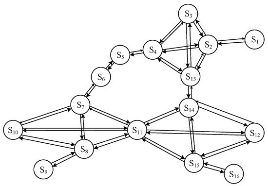
Figure 2.
An example of a segment graph.
(6) Traffic State
The traffic state is used to describe the state of a segment and is defined as follows:
where is the identifier of the segment; and denote the start time and end time of this traffic state, respectively; v denotes the average velocity of the segment; and describes traffic jam , traffic control , slow-moving , free-moving and traffic event information .
(7) Route
A route represents conceptual entities in the real world, such as expressways, ramps or highways and is defined as follows:
where is the identifier of the route, and and denote the name and length, respectively. The flags and are similar to the definition of segment. Note that does not include the geometry to save storage.
(8) Route Graph
A route graph structure is composed of set of nodes (routes) and edges . It is defined as:
The relationship includes two types of edges and is defined as follows:
where represents a set of spatial relationships between two routes and represents the fact that a route includes a set of segments. Figure 3 shows an example of a route graph of a road network (as shown in Figure 1). The route includes three segments: , and .
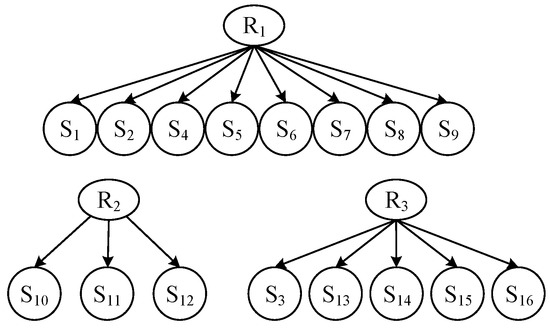
Figure 3.
An example of a route graph.
3.4. Moving Object Representation
is used to represent moving objects and is composed of a set of objects and a set of social relationships between moving objects, such as friendship and colleague.
(9) Moving Object
A moving object is defined as:
where and are the identification and name of a moving object, and refers to other attribute sets.
(10) Object Graph
An object graph structure is used to model moving objects and the social relationships between them. It is defined as follows:
where denotes moving objects and denotes the social relationships between two moving objects:
The represents social relationships between moving objects, including colleagues, friendships, followership, interest group and fan relationships.
(11) Object’s Position
A moving object’s position represents a moving object’s relative position in a certain segment and absolute coordinates. It is defined as follows:
where is the identifier of the segment, denotes the object’s geospatial coordinates and d describes the position of the moving object in the network relative to distance markers on the roads.
3.5. Trajectory Representation
We use MoveGraph to represent the trajectories of moving objects.
(12) Moving Vector
is used to model an object’s moving vector at time t and is defined as follows:
where is the identifier of a moving object, v denotes the instantaneous velocity at time t and denotes the object’s relative position in a certain segment.
(13) Trajectory Unit
We aggregate all location points of a moving object in the current segment as a trajectory unit . It is defined as follows:
where is the identifier of the segment and is the identifier of the moving object.
(14) Trajectory
A moving object’s trajectory could be represented as a collection of trajectory units and is defined as follows:
(15) Move Graph
A move graph structure is defined to represent the trajectories of moving objects and includes a set of nodes (trajectory units) and edges (relationships between trajectory units). It is defined as:
The relationship is defined as follows:
where represent the ordinal relationships between trajectory units that belong to the same trajectory. They help to easily retrieve the entire trajectory of a moving object. represent the relationships between a trajectory unit and a moving object , and represent the relationships between trajectory unit and segment . These relationships provide the capability to find all trajectories in a specific segment. Meanwhile, we also could retrieve all trajectories in a specific route with the help of edges .
Figure 4 illustrates an example of a move graph. As shown in the figure, the trajectory of a moving object includes three trajectory units and moves through three segments.
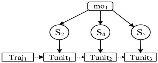
Figure 4.
An example of a move graph.
4. Operators
In this section, we consider the interaction between networks, trajectories and semantic information and propose a large set of operators, as shown in Table 1. To define operations in a generic way, we use the signature to illustrate operators’ signatures and semantics. That means the data type variables α and β could be instantiated; for example, is used to multiply two real numbers.

Table 1.
Definition of operations.
(1) Select
The operator returns all moving objects that meet the query condition, such as the field value of moving objects’ attributes. For instance, to find a vehicle with license ‘B-YI 65’ over a object graph , the query expression is written as:
(2) nodevalues
The operator gets a field’s value of the moving objects’ attribute. For instance, we want to retrieve a vehicle’s model of moving object ; the query expression is written as:
(3) getnodes
The operator returns all adjacent moving objects, segments or trajectory units, according to a specific relationship value. For instance, the following expression means to retrieve all segments for which the object is moving.
(4) getrajectory
The operator retrieves trajectories of a moving object at specific date . For instance, we want to find all trajectories of a vehicle with license ‘B-YI 65’ on 22 January 2017; it is written as:
(5) getsegments
The operator traverses all segments in networks to retrieve the specific segment that corresponds to the input network location .
(6) getmos
The operator retrieves all moving objects that are passing through the input network location .
(7) getlen
The operator calculates the length of a trajectory unit .
(8) atinstants
The operator retrieves any position of a moving object at time . This operator requires the interpolated operation of the trajectory between two adjacent points because of the trajectories’ discreteness. For instance, a query ‘where is the vehicle with license ‘B-YI 65’ at 10:00 on 22 January 2017?’ can be written as:
(9) atperiods
The operator retrieves all trajectory units that satisfy the query time condition and the specific trajectory .
(10) exinstants
The operator performs the reverse operation of the . It will receive coordinate information and returns the time when the moving object passes through it.
(11) distance
The operator retrieves the minimum Euclidean distance between two trajectories . It will calculate all distance values from a point of the first trajectory to any points of another trajectory. Then, it returns the minimum distance value.
5. Benchmark Queries
In this section, we perform a set of interesting benchmark queries that were written in common natural language to test the performance and efficiency of our proposed GSMNet model. The benchmark queries should not only demonstrate the strengths, but also the weaknesses of the data model; we employ a recognized benchmark BerlinMOD [24] that builds on Secondo database management system (DBMS)to compare the performance of different spatio-temporal database management systems. It identifies 96 query types according to five query properties: object identity, dimension, query interval, condition type and aggregation. However, not all of the query types are interesting for benchmark queries. Seventeen carefully selected benchmark queries are presented according to systematic analysis and combinations, as shown in Table 2. We formulate these queries in formal SQL-like notation based on the proposed data types and operators in the GSMNet model.
Table 2.
Seventeen benchmark queries.
First, we introduce many common database objects in BerlinMOD to better understand the meaning and semantics of these queries. QueryPoints represent the query points and are defined as , where is the identification for this relation, denotes the query coordinates and is the data type provided by Secondo [14,36,37]. QueryRegions are defined as , where is a key and are regular regions. QueryInstants are defined as , and QueryPeriods are defined as . QueryLicences denote the license plate numbers that are sampled from all vehicles and are represented as . BerlinMOD adopts two types of data model: the Object-Based Approach (OBA) and the Trip-Based Approach (TBA). For the OBA, the entire trajectory is kept together. For the TBA, the entire trajectory is divided into a sequence of trips.
For simplicity, we only provide our implementation based on the proposed GSMNet model, as follows. For the formulation of queries in BerlinMOD, refer to the literature [24].
Query 1: What are the models of vehicles with license plate numbers from QueryLicences ?
This query mainly tests the performance on standard data types , standard operators and and the standard index on licence. Compared with TBA and OBA approaches, this query only traverses the ObjectGraph in the GSMNet model to produce the query answer. The strategy that aggregates all moving objects into a single subgraph structure could efficiently avoid performance degradation because of the increase of the the trajectories’ data scale. This is important for significantly improving query performance.
Query 2: How many vehicles exist that are ‘passenger’ cars?
This query also tests the standard data types , operators and the aggregation operators . High query performance also benefits from the hierarchical graph design in the GSMNet model, and the index on the attribute Type field could make it perform better.
Query 3: Where have the vehicles with licenses from QueryLicences1 been at each of the instants from QueryInstants1?
This query needs to retrieve a specific position of the moving objects at query instants. First, the GSMNet model adopts the operator to locate all objects that satisfy the query condition QueryLicences1. This step benefits from the index on the licence field. Then, the operator retrieves the corresponding trajectories of the query objects. The time operator intercepts it at a query instant. Finally, the road segment nodes are retrieved by the operator .
Query 4: Which license plate numbers belong to vehicles that have passed the points from QueryPoints?
This query mainly tests the performance of the spatial index on the trajectories. The operator traverses MoveGraph to find the trajectory unit that pass the QueryPoints.
Query 5: What is the minimum distance between places, where a vehicle with a license from QueryLicences1and a vehicle with a license from QueryLicences2 have been?
First, this query needs to find corresponding moving objects quickly using the index on the licence field. Then, it retrieves the objects’ trajectories using the operator . The operator calculates the distance between two trajectories.
Query 6: What are the pairs of license plate numbers of ‘trucks’ that have ever been as close as 10 m or less to each other?
Because the complexity of this query is , the execution time grows quickly as the number of trucks increases. The index on the type field appears to be helpful. The operator is important for influencing the efficiency of this query.
Query 7: What are the license plate numbers of the ’passenger’ cars that have reached the points from QueryPoints first out of all ’passenger’ cars during the complete observation period?
This query first needs to locate all moving passenger cars in ObjectGraph and obtain all trajectories using the operator . Then, this query extracts the time that objects pass the input query points using the operator . The operator returns the time that objects first pass the points. Finally, this query uses the operator to find corresponding moving objects’ nodes.
Query 8: What are the overall traveled distances of the vehicles with license plate numbers from QueryLicences1 during the periods from QueryPeriods1?
This query uses the operator to extract moving objects’ trajectory segments during the query periods. The operator length calculates the travel distances of moving objects. The index on licence is helpful.
Query 9: What is the longest distance that was traveled by a vehicle during each of the periods from QueryPeriods?
This query is similar to Query 8. It needs to retrieve all of the vehicle’s trajectories and then extract the trajectory segments during the query periods. The operator determines the longest travel distance.
Query 10: When and where did the vehicles with license plate numbers from QueryLicences1 meet other vehicles (distance <3 m), and what are the latter’s licenses?
This query also belongs to a complex query that is similar to Query 6. It needs to determine the accurate location and time that the two vehicles meet each other.
Query 11: Which vehicles passed a point from QueryPoints1 at one of the instants from QueryInstants1?
This query mainly tests the performance of the spatial index. It needs to determine all trajectories for which vehicles passed the query points using the spatial index on the GEOM. Then, the operator retrieves the corresponding locations. This query uses the operator to locate moving objects that pass the query points.
Query 12: Which vehicles met at a point from QueryPoints1 at an instant from QueryInstants1?
This query is very similar to Query 11. It needs to determine whether there are two vehicles that meet at query points at query instants using operator .
Query 13: Which vehicles traveled within one of the regions from QueryRegions1 during the periods from QueryPeriods1?
This query tests the performance of the time index and spatial index. The two indices enhance the efficiency of this query.
Query 14: Which vehicles traveled within one of the regions from QueryRegions1 at one of the instants from QueryInstants1?
Unlike Query 13, this query needs to use the operator to obtain corresponding trajectories that travel within query regions.
Query 15: Which vehicles passed a point from QueryPoints1 during a period from QueryPeriods1?
This query also tests the performance of the spatial index and time index.
Query 16: List the pairs of licenses for vehicles, the first from QueryLicences1, the second from QueryLicences2, where the corresponding vehicles are both present within a region from QueryRegions1 during a period from QueryPeriod1, but do not meet each other there and then.
This query first locates all moving vehicles’ trajectories and then determines whether the trajectory and query regions intersect using the operator . The operator retrieves trajectory segments during the query periods. Then, the query uses the operator to determine pairs of licenses for vehicles.
Query 17: Which points from QueryPoints have been visited by a maximum number of different vehicles?
This query benefits from the GSMNet model at the extreme because the query could easily retrieve all trajectories’ segments that move in a specific segment through the edge from the trajectory node to segment node.
6. Experiments
6.1. Experimental Settings
The proposed GSMNet model was implemented using Java as the main programming language and Eclipse 4.4.1 as the development environment. The experiments were conducted on a virtual machine, SecondoVM with Intel i7-4790 CPU, 2G RAM and 20 G mechanical hard disk, which was a Linux-based installation of the Secondo extensible DBMS and provided on the web. Ubuntu 11.10 was installed as the operating system, with Secondo DBMS and BerlinMOD Benchmark. The experimental data were pre-generated BerlinMOD data with different scale factors 0.05, 0.2 and 0.1. The parameter is the global factor of BerlinMOD that determines the amount of data generated. Table 3 illustrates the detailed information of experimental dataset for different scalefactor values. As shown in the table, we can see that the scale of data grows explosively; for scale factor 1.0, the size of the data is about 11 GB, and the number of trips is 292,940. Hence, the experiments have enough data to evaluate the computational performance of our proposed GSMNet model. Figure 5 shows the spatial distribution of a different number of trajectories. The dataset was directly downloaded from the Secondo website in CSV format. The files included datamcar.csv, trips.csv, queryinstants.csv, querylicences.csv, queryperiods.csv, querypoints.csv, queryregions.csv and streets.csv.
Table 3.
Experimental data.
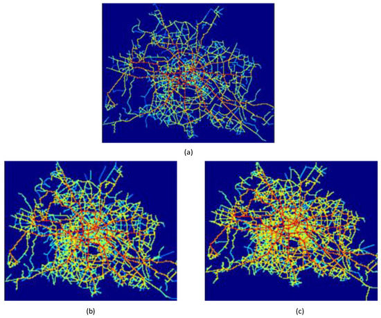
Figure 5.
Heat Map of Experimental Data with Different Scalefactors: scalefactor 0.05 (a), scalefactor 0.2 (b) and scalefactor 1.0 (c).
6.2. Experimental Results
We repeated the benchmark query execution several times for both approaches. Table 4 and Figure 6 compare the average query run times in seconds for the proposed GSMNet model and Secondo for different , data models and approaches.
Table 4.
Benchmarking the Geo-Social-Moving model for moving objects in Networks (GSMNet) model using the Berlin Moving Objects Database (BerlinMOD) in seconds. OBA, Object-Based Approach; TBA, Trip-Based Approach.
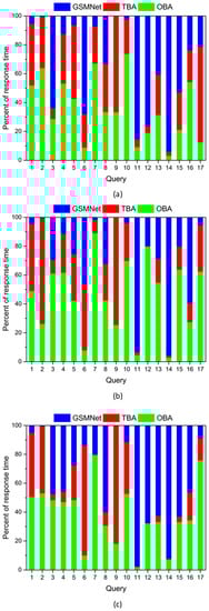
Figure 6.
Comparison of GSMNet and Secondo with Different Scalefactors: scalefactor 0.05 (a), scalefactor 0.2 (b) and scalefactor 1.0 (c).
For Queries 1 and 2, GSMNet outperformed TBA and OBA for the different , and the query run times were almost the same for different numbers of trajectories. An index on Licence was useful to improve the performance. The results show that our implementation has reliable performance on standard types and indices.
For Query 3, GSMNet was faster than TBA, but slower that OBA. This result was expected because the number of trajectory units in GSMNet and TBA was greater than the number of units in OBA. Therefore, the query implementation in OBA could quickly be restricted to single query instants. However, compared with TBA, GSMNet easily retrieved the entire trajectories through the relationships and saved a great deal of query run time. Both approaches were benefit from indexes on Licence.
GSMNet outperformed TBA and OBA for Queries 4 and 5 because it benefited from the relationships pointing from trajectory unit to road segment . Therefore, GSMNet could easily retrieve all trajectories’ units that passed the query points in road segments. That also reflects that GSMNet characterized by graph traversal has strong potential to reduce time-consuming table join operations in traditional approaches.
For Query 6, OBA outperformed GSMNet and TBA for all amounts of data. This query first needed to select candidate trucks and then compare all corresponding trajectories’ units. Because the number of units in TBA and GSMNet was greater than the number of units in OBA, the query required slightly less time in OBA than in TBA and GSMNet.
GSMNet outperformed OBA for Query 7. In GSMNet, we retrieved a candidate passenger from object graph and determined all of the query points from segment graph . The relationships between trajectory unit and road segment helped us to retrieve all trajectories’ units. Then, the query determined if there were relationships between a trajectory unit and moving object .
The classical Query 8 needed to calculate the distance of trajectories, and it was a fast query in TBA, OBA and GSMNet. However, GSMNet loses at 1.0 because the number of trajectories’ units in GSMNet was greater than the other approaches.
The good result from Query 9 exceeded our expectations. This query summed the lengths of all trajectories and returned the longest distance. In GSMNet, the relationship retrieved all trajectory units ; mainly because the length of trajectory unit is pre-computed. Hence, this query in GSMNet only summed the lengths of trajectory units. Therefore, it saved a great deal of time.
For complex Query 10, GSMNet outperformed TBA and OBA. This query needed to simultaneously consider both the temporal and spatial distance. The advantage of GSMNet is that we used many relationships to connect moving objects, road segments and trajectories’ units. However, TBA and OBA required many time-consuming aggregation operations in this query.
Query 11 is similar to Query 12. However, we did not expect that GSMNet would be slower than TBA and OBA. In the experiments, the spatial index on the trip and temporal index on query instants in TBA and OBA played an important part in the improvement of efficiency. By contrast, GSMNet still first retrieved the corresponding road segments from query points. Then, we used the relationships between trajectory unit and road segment to determine all candidate trajectory units. Many loops through the trajectory units were performed to determine if candidates met the query instants run more times than the spatial-temporal index.
Queries 13, 14 and 15 focused on testing the performance of spatial-temporal indices. TBA and OBA outperformed GSMNet because our implementation used the relationships and to substitute for the spatial indices.
For Queries 16 and 17, the performance of GSMNet was in line with our expectations. The number of trajectory units had a significant impact on performance.
In our experiments, we have detected some points of the strengths and weaknesses in the GSMNet model by comparison with the most mature moving objects database Secondo. The pairwise comparison results show that GSMNet has higher efficiency in several queries involving more table-join operations, such as Queries 3, 5, 7, 9, 10, 16, 17. The weakness of GSMNet occurs in queries with a large data scale. For example, when the number of trips is 292,940 at scalefactor 1.0, GSMNet shows signs of performance degradation in Queries 11, 12, 14. However, Secondo performs high stability.
6.3. Discussion
(1) The proposed GSMNet model has the capability of representing semantic information, including traffic state and social relationships. To keep contrasting experiments at the same starting point, the standard 17 benchmark queries remained relatively untouched, although they involved a small amount of semantic information in the experiments. However, the experimental results show that the performance of our proposed GSMNet is workable and reliable. The benchmark queries could also be easily extended to cover semantic information. For example, we could add social relationships to Query 12, in which vehicles met their friends at a point from QueryPoints1 at an instant from QueryInstants1. More experiments containing semantic information need to be performed in the future. Meanwhile, GSMNet should be extended to represent more semantics, for instance human behavior information, including group behavior and individual behavior, such as herd, swarm, convoy pattern and moving clusters.
(2) Graph structures are widely used to represent road networks. However, the proposed GSMNet model innovatively adopted two dual graph structures to model the network at different levels of granularity. The advantage is that traffic information could be easily integrated into the model and the topological relationships between routes and segments could be represented as edges. Additionally, GSMNet also represents trajectories and moving objects’ social relationships as graph structures, thus enabling the integration of spatial and semantic information. Based on this design, uniform graph traversal operations could be used to substitute time-consuming table join operations, as shown in the experimental results of Queries 4 and 5.
(3) The proposed GSMNet model mainly focuses on modeling massive trajectories and the underlying road networks. However, benefiting from the design of the proposed GSMNet model, it can be finely tuned to support the representation of other activity environments, such as indoor or geographical free spaces [38]. However, storing too much information through the attributes of nodes or edges will make the graphs overstaffed or redundant and cause performance degradation. The experimental results reflect the weakness of the proposed GSMNet model. The efficiency of benchmark queries all decreased at 1.0. Compressing the trajectories and storing the attributes of graph nodes or edges with a binary system may be a useful strategy for solving the problem.
7. Conclusions
In this paper, we proposed a hierarchical graph model GSMNet for moving objects in networks for the integrated representation of moving objects, trajectories, underlying networks and semantic information, including traffic states and social relationships between moving objects. GSMNet has the capability of flexibly balancing the cost of location updates and the granularity of modeling underlying networks with the help of the multi-level representation of RouteGraph and SegmentGraph. Additionally, we developed a data type system and provided formal definitions of corresponding operators of the GSMNet model. Seventeen benchmark queries was conducted using the GSMNet model. Compared with Secondo, we argued that our proposed GSMNet model was more general and efficient. It is a good attempt toward enhancing integrated spatial-temporal data modeling for moving objects in networks because shifting from raw trajectories to semantic trajectories is a general trend.
Several directions for future work are worthy of attention. First, our proposed GSMNet model has only been applied to moving objects in network environments. The extension of the proposed data model to other environments, such as indoors, is an interesting topic for future work. Another topic is to implement parallel processing of the proposed GSMNet model to accelerate query performance in distributed computing environments using a large-scale graph commutating processing framework, such as Pregel and the Bulk Synchronous Parallel (BSP) model; Second, multiple types of spatial-temporal queries based on the proposed GSMNet model, such as range queries, kNN queries and skyline queries, are an interesting research issue; Last, but not least, future studies will address trajectory data mining issues based on the proposed GSMNet model, including trajectory pattern mining and trajectory clustering methods.
Acknowledgments
This research was supported by the National Natural Science Foundation of China (Grant No. 41401460) and the State Key Research Development Program of China (Grant No. 2016YFB0502104). We also thank the anonymous referees for their helpful comments and suggestions.
Author Contributions
Hengcai Zhang and Feng Lu provided the core idea for this study and designed the experiments; Hengcai Zhang performed the experiments; Hengcai Zhang and Feng Lu analyzed the data; Hengcai Zhang and Feng Lu wrote the paper.
Conflicts of Interest
The authors declare no conflict of interest.
References
- Pelekis, N.; Theodoridis, Y. Mobility Data Management and Exploration; Springer: New York, NY, USA, 2014; pp. 75–99. [Google Scholar]
- Zheng, Y. Trajectory Data Mining: An Overview. ACM Trans. Intell. Syst. Technol. 2015, 6, 29–48. [Google Scholar] [CrossRef]
- Hajari, H.; Hakimpour, F. A Spatial Data Model for Moving Object Databases. Int. J. Database Manag. Syst. 2014, 6, 1–20. [Google Scholar] [CrossRef]
- Kanjilal, V.; Schneider, M. Spatial Network Modeling for Databases. In Proceedings of the 2011 ACM Symposium on Applied Computing, TaiChung, Taiwan, 21–24 March 2011; pp. 827–832.
- Buonanno, A.; D’Urso, M.; Prisco, G.; Felaco, M.; Meliadó, E.; Mattei, M.; Palmieri, F.; Ciuonzo, D. Mobile Sensor Networks Based on Autonomous Platforms for Homeland Security. In Proceedings of the 2012 Tyrrhenian Workshop on Advances in Radar and Remote Sensing (TyWRRS), Naples, Italy, 12–14 September 2012; pp. 80–84.
- Brooks, R.R.; Ramanathan, P.; Sayeed, A.M. Distributed Target Classification and Tracking in Sensor Networks. Proc. IEEE 2003, 91, 1163–1171. [Google Scholar] [CrossRef]
- Ciuonzo, D.; Buonanno, A.; D’Urso, M.; Palmieri, F.A. Distributed Classification of Multiple Moving Targets with Binary Wireless Sensor Networks. In Proceedings of the 14th International Conference on Information Fusion, Chicago, IL, USA, 5–8 July 2011; pp. 1–8.
- D’Costa, A.; Ramachandran, V.; Sayeed, A.M. Distributed Classification of Gaussian Space-time Sources in Wireless Sensor Networks. IEEE J. Sel. Areas Commun. 2004, 22, 1026–1036. [Google Scholar] [CrossRef]
- Huang, S.-C.; Chen, B.-H. Highly Accurate Moving Object Detection in Variable Bit Rate Video-based Traffic Monitoring Systems. IEEE Trans. Neural Netw. Learn. Syst. 2013, 24, 1920–1931. [Google Scholar] [CrossRef]
- Huang, S.-C.; Jiau, M.-K.; Hsu, C.-A. A High-efficiency and High-accuracy Fully Automatic Collaborative Face Annotation System for Distributed Online Social Networks. IEEE Trans. Circuits Syst. Video Technol. 2014, 24, 1800–1813. [Google Scholar] [CrossRef]
- Cheng, F.-C.; Chen, B.-H.; Huang, S.-C. A Hybrid Background Subtraction Method with Background and Foreground Candidates Detection. ACM Trans. Intell. Syst. Technol. 2015, 7, 141–160. [Google Scholar] [CrossRef]
- Yan, T.; Zhang, W.; Wang, G. DOVE: Data Dissemination to A Desired Number of Receivers in VANET. IEEE Trans. Veh. Technol. 2014, 63, 1903–1916. [Google Scholar] [CrossRef]
- Yan, T.; Zhang, W.; Wang, G.; Zhang, Y. Access Points Planning in Urban Area for Data Dissemination to Drivers. IEEE Trans. Veh. Technol. 2014, 63, 390–402. [Google Scholar] [CrossRef]
- Güting, R.H.; Ding, Z. Modeling and Querying Moving Objects in Networks. VLDB J. 2006, 15, 165–190. [Google Scholar] [CrossRef]
- Parent, C.; Spaccapietra, S.; Renso, C.; Andrienko, G.; Andrienko, N.; Bogorny, V.; Damiani, M.L.; Gkoulalas-Divanis, A.; Macedo, J.; Pelekis, N. Semantic Trajectories Modeling and Analysis. ACM Comput. Surv. 2013, 45, 111–120. [Google Scholar] [CrossRef]
- Schneider, M. Moving Objects in Databases and GIS: State-of-the-Art and Open Problems. In Research Trends in Geographic Information Science; Springer: Berlin/Heidelberg, Germany, 2009; pp. 169–187. [Google Scholar]
- Wolfson, O.; Chamberlain, S.; Kalpakis, K.; Yesha, Y. Modeling Moving Objects for Location Based Services. In Developing an Infrastructure for Mobile and Wireless Systems; Springer: Berlin/Heidelberg, Germany, 2002; pp. 46–58. [Google Scholar]
- Xu, J.; Güting, R.H.; Zheng, Y. The TM-RTree: An Index on Generic Moving Objects for Range Queries. GeoInformatica 2015, 19, 487–524. [Google Scholar] [CrossRef]
- Hu, W.; Yang, Y.; Zhang, W.; Xie, Y. Moving Object Detection Using Tensor-Based Low-Rank and Saliently Fused-Sparse Decomposition. IEEE Trans. Image Process. 2017, 26, 724–737. [Google Scholar] [CrossRef] [PubMed]
- Ding, Z.; Güting, R. Modeling Temporally Variable Transportation Networks. Database Syst. Adv. Appl. 2004, 2973, 651–724. [Google Scholar]
- Ding, Z.; Güting, R.H. Managing Moving Objects on Dynamic Transportation Networks. In Proceedings of the 16th International Conference on Scientific and Statistical Database Management, Santorini Island, Greece, 21–23 June 2004; pp. 287–296.
- Chen, J.; Meng, X.; Guo, Y.; Grumbach, S.; Sun, H. Modeling and Predicting Future Trajectories of Moving Objects in A Constrained Network. In Proceedings of the 7th International Conference on Mobile Data Management (MDM’06), Nara, Japan, 10–12 May 2006; p. 156.
- Qi, L.; Schneider, M. MONET: Modeling and Querying Moving Objects in Spatial Networks. In Proceedings of the Third ACM SIGSPATIAL International Workshop on GeoStreaming, Redondo Beach, CA, USA, 7–9 November 2012; pp. 48–57.
- Düntgen, C.; Behr, T.; Güting, R.H. BerlinMOD: A Benchmark for Moving Object Databases. VLDB J. 2009, 18, 1335–1368. [Google Scholar] [CrossRef]
- Chen, B.Y.; Yuan, H.; Li, Q.; Lam, W.H.; Shaw, S.-L.; Yan, K. Map-matching Algorithm for Large-scale Low-frequency Floating Car Data. Int. J. Geogr. Inf. Sci. 2014, 28, 22–38. [Google Scholar] [CrossRef]
- Chou, S.-K.; Jiau, M.-K.; Huang, S.-C. Stochastic Set-Based Particle Swarm Optimization Based on Local Exploration for Solving the Carpool Service Problem. IEEE Trans. Cybern. 2016, 46, 1771–1783. [Google Scholar] [CrossRef] [PubMed]
- Huang, S.-C.; Chen, B.-H. Automatic Moving Object Extraction through A Real-world Variable-bandwidth Network for Traffic Monitoring Systems. IEEE Trans. Ind. Electron. 2014, 61, 2099–2112. [Google Scholar] [CrossRef]
- Jensen, C.S.; Kolářvr, J.; Pedersen, T.B.; Timko, I. Nearest Neighbor Queries in Road Networks. In Proceedings of the 11th ACM International Symposium on Advances in Geographic Information Systems, New Orleans, LA, USA, 3–8 November 2003; pp. 1–8.
- Shekhar, S.; Yoo, J.S. Processing In-Route Nearest Neighbor Queries: A Comparison of Alternative Approaches. In Proceedings of the 11th ACM International Symposium on Advances in Geographic Information Systems, New Orleans, LA, USA, 3–8 November 2003; pp. 9–16.
- Vazirgiannis, M.; Wolfson, O. A Spatiotemporal Model and Language for Moving Objects on Road Networks. In Proceedings of the 7th International Symposium on Advances in Spatial and Temporal Databases, Redondo Beach, CA, USA, 12–15 July 2001; pp. 20–35.
- Speičvcys, L.; Jensen, C.S.; Kligys, A. Computational Data Modeling for Network-Constrained Moving Objects. In Proceedings of the 11th ACM International Symposium on Advances in Geographic Information Systems, New Orleans, LA, USA, 3–8 November 2003; pp. 118–125.
- Xu, J.; Güting, R.H. A Generic Data Model for Moving Objects. Geoinformatica 2013, 17, 125–172. [Google Scholar] [CrossRef]
- Chen, B.Y.; Yuan, H.; Li, Q.; Shaw, S.-L.; Lam, W.H.; Chen, X. Spatiotemporal Data Model for Network Time Geographic Analysis in The Era of Big Data. Int. J. Geogr. Inf. Sci. 2016, 30, 1041–1071. [Google Scholar] [CrossRef]
- Ding, Z.; Yang, B.; Güting, R.H.; Li, Y. Network-matched Trajectory-based Moving-object Database: Models and applications. IEEE Trans. Intell. Transp. Syst. 2015, 16, 1918–1928. [Google Scholar] [CrossRef]
- Ding, Z.; Yang, B.; Chi, Y.; Guo, L. Enabling Smart Transportation Systems: A Parallel Spatio-Temporal Database Approach. IEEE Trans. Comput. 2016, 65, 1377–1391. [Google Scholar] [CrossRef]
- Güting, R.H.; Böhlen, M.H.; Erwig, M.; Jensen, C.S.; Lorentzos, N.A.; Schneider, M.; Vazirgiannis, M. A Foundation for Representing and Querying Moving Objects. ACM Trans. Database Syst. 2000, 25, 1–42. [Google Scholar] [CrossRef]
- Güting, R.H.; Almeida, V.; Ansorge, D.; Behr, T.; Ding, Z.; Höse, T.; Hoffmann, F.; Spiekermann, M.; Telle, U. SECONDO: An Extensible DBMS Platform for Research Prototyping and Teaching. In Proceedings of the 21st International Conference on Data Engineering (ICDE’05), Tokyo, Japan, 5–8 April 2005; pp. 1115–1116.
- Zhang, H.; Lu, F.; Xu, J. Modeling and Querying Moving Objects with Social Relationships. ISPRS Int. J. Geo-Inf. 2016, 5, 121. [Google Scholar] [CrossRef]
© 2017 by the authors. Licensee MDPI, Basel, Switzerland. This article is an open access article distributed under the terms and conditions of the Creative Commons Attribution (CC BY) license ( http://creativecommons.org/licenses/by/4.0/).