
Optimizing Multi-Way Spatial Joins of Web Feature Services

1
College of Geomatics and Geoinformation, Guilin University of Technology, Guilin 541004, China
2
Guangxi Key Laboratory of Spatial Information and Geomatics, Guilin 541004, China
*
Author to whom correspondence should be addressed.
ISPRS Int. J. Geo-Inf. 2017, 6(4), 123; https://doi.org/10.3390/ijgi6040123
Submission received: 29 November 2016
/
Revised: 8 April 2017
/
Accepted: 14 April 2017
/
Published: 20 April 2017
(This article belongs to the Special Issue Recent Advances in Geodesy & Its Applications)
Abstract
:Web Feature Service (WFS) is a widely used spatial web service standard issued by the Open Geospatial Consortium (OGC). In a heterogeneous GIS application, a user can issue a query that relates two or more spatial datasets at different WFS servers. Multi-way spatial joins of WFSs are very expensive in terms of computation and transmission because of the time-consuming interactions between the servers and the client. In this paper, we examine the problems of multi-way spatial joins of WFSs, and we present a client-side optimization approach to generate good execution plans for such queries. The spatial semi-join and area partitioning-based methods are combined to prune away non-candidate objects in processing binary spatial joins, and the filtering rate is used as an index to determine the execution strategy for each sub-area. Two partitioning methods were tested, and the experimental results showed that both are effective if a proper threshold to stop the partitioning is chosen. In processing multi-way spatial joins of WFSs, the filtering rate is used as an indicator to determine the ordering of the binary joins. The optimization method is obviously superior to the other two methods when there are adequate spatial objects involved in the join query, or when more datasets are involved in the join query.
1. Introduction
Spatial information at present is widely utilized in many decision-making processes. Many application domains, such as emergency and disaster management, necessitate the analysis of spatial data that are geographically distributed [1]. In recent years, the OGC (Open Geospatial Consortium) has released a series of OpenGIS Implementation Specifications that serve as one of the solutions to spatial data interoperability and sharing. As one of the geospatial web service standards, Web Feature Service (WFS) [2,3] provides transactions on and access to geographic information over the HTTP protocol at the feature and feature property level in a manner that is independent of the underlying data store. The WFS standard now has been implemented in a number of mainstream GIS webservers, such as ArcGIS Server, Deegree and Geoserver, among others. Progress in this aspect of the GIS industry makes it possible to build GIS applications that integrate spatial data managed by different GIS platforms, from different departments/agencies [4]. The well-known open-source project, OpenLayers (http://openlayers.org) has provided some modules that support access to WFSs and dynamic maps. There have been some WebGIS applications that use WFSs as a type of data sources, such as Land and Resources Management Systems [5], Disaster Response System [6,7] and Logistics Information Systems [8]. Obviously, WFS has become very promising in the integrated application of spatial data [9].
In heterogeneous spatial data applications, the answers to some queries may often involve integrating and analyzing data from a number of services [10,11,12]. For example, the solution to the query “which schools are less than 1 km from a police station?” could require processing a spatial join between two WFSs if the dataset “school” and “police station” are provided by two data providers. Because spatial data are encoded in geography markup language (GML) when transferred between a WFS server and its client, generating a GML document on the server and parsing it on the client is expensive in terms of the computation and transmission costs. In traditional spatial database management systems (DBMSs) [13], even with the help of spatial index techniques, it is very expensive to process spatial joins, in terms of both CPU and I/O cost. Comparatively, it would be more time consuming to process multi-way spatial joins (MSJ) of WFSs due to the expensive interactions between the servers and their clients, especially when clients have no access to the spatial indices on the servers. Therefore, it is necessary to find some better methods to reduce the overhead for this type of spatial join query. Multi-way spatial joins of WFSs can be seen as a type of special distributed spatial join, and therefore, to a certain extent, the existing optimization methods for the latter will be of help in searching for solutions for this issue. To accelerate the response of client applications, there have been a number of server-side optimization methods, such as creating a spatial index for datasets that are frequently accessed or reducing the redundant GML elements in GML documents by optimizing the definitions of GML application schemas of the datasets [9]. From the client’s point of view, a quicker response to the users can be expected not only by optimization on the servers accessed but also by the optimization strategies utilized on the client side itself. Currently, very few research studies have been conducted on optimizing this type of spatial join on the client side, and existing research on MSJ has largely focused on generating optimal execution plans for traditional centralized or distributed spatial DBMSs [13,14,15,16]. In our previous work, we have attempted to reduce the transmission cost of spatial joins of two WFSs [17,18]. In this research, we aimed at developing a client-side optimization approach to generate an optimal execution plan for MSJ of WFSs.
2. Multi-Way SPATIAL Join of Web Feature Services
In this section we firstly give a formal definition of the distributed multi-way spatial join, and introduce the interaction mode between WFSs and their client. Then we introduce the related research on MSJ in traditional spatial DBMSs. Last, some issues on processing MSJs of WFSs are introduced and discussed.
2.1. Open Geospatial Consortium (OGC) Web Feature Service
The international standard of Web Feature Service specifies the behaviour of a service that provides transactions on and access to geographic features in a manner that is independent of the underlying data store [3]. A WFS must respond to a client’s request according to the implementation specification. As a self-descriptive agent, a WFS supports a GetCapabilities operation and a DescribeFeatureType operation. The GetCapabilities operation generates a service metadata document, and the DescribeFeatureType operation returns a schema description of the feature types offered by a WFS instance; with the metadata served by the two operations, the client can discover what it provides and know how to access the spatial data from the WFS server. The GetFeature operation allows a client to retrieve spatial features or values of feature properties from the data store of the WFS. In a GetFeature request, there is a parameter called “resultType.” The WFS can respond to this request in one of two ways according to the value of the resultType parameter. If the resultType is set to “results,” the service will return a complete document that contains all the features that satisfy the query expressions; otherwise, if it is set to “hits,” the service simply returns the total number of selected features.
The cost of a WFS request and its response involves at least the following aspects: (1) the client sends the query request to the server; (2) the server performs a query operation to obtain the qualified spatial objects; (3) the server transforms the query result into GML format; (4) the server transfers the GML document to the client; and (5) the client receives the GML document and parses it. We used a dataset called tl_2015_us_ rails, one of the 2015 TIGER/Line provided by the United States Census Bureau, to determine the time costs of these steps. In this experiment, ten portions of tl_2015_us_ rails with different data sizes were selected and encoded into XML format on the server before being transmitted to the client side and parsed. More information about our experiment will be introduced in Section 4. Table 1 shows the time costs of the above steps. In Table 1, DS_SHF is the data size in shapefile format; DS_XML is the data size in XML format; ENCODE_T is the time cost of the request and query operation and encoding the results into XML format; PARSE_T is the time cost of parsing the responded XML document; and TOTAL is the time cost of the whole process.
Table 1 shows that the time costs of these steps are approximately proportional to the original data sizes in the shapefile format. TRANS_T was not dominant because in this experiment, the client and the server were connected by a local area network, with a sustained data transfer rate of approximately 30 Mbps. It can be confirmed that TRANS_T would increase if the experiment was conducted under the circumstances of the Internet. Comparatively speaking, a request with the parameter resultType being set to “hits” is less susceptible to the data transfer rate because it only requires transferring the number of selected features. Accordingly, it needs around 1/20 of the time cost of the corresponding query that returns all the qualified objects in XML format; most time is spent on searching for and counting these objects in the server’s database. In this study, we used this type of query to estimate spatial distributions of joined datasets.
2.2. Multi-Way Spatial Join
The multi-way spatial join implicates an arbitrary number of spatial datasets [13]. Formally, a multi-way spatial join can be depicted as follows. Given that R is a collection of datasets, , , with the ith dataset in R, for an arbitrary pair of datasets and , the join query between them can be defined as , where is the spatial predicate that should be held between and . A multi-way spatial join can be viewed as an undirected graph , where the nodes correspond to the datasets, and the edges to the join predicates. Let be an arbitrary element in the adjacency matrix of the query graph; then, denotes that there is a spatial join between the datasets and . Otherwise, if , and are not joined.
In traditional spatial DBMSs, spatial index techniques are widely used in spatial join processing. Several non-index methods have also been proposed for binary spatial join processing, such as Spatial Hash Join [19], Partition-Based Spatial–Merge Join [20], Scalable Weeping-Based Spatial Join [21], and Iterative Spatial Join [22]. The methods for processing MSJs can be grouped into two categories. The first method is to search for tuples satisfying the query from datasets all at once, such as synchronous traversal (ST) [23]. To avoid an exhaustive search or false hits, these methods require the joined datasets to be indexed [13]. The second way is to decompose the whole query into a sequence of binary joins, which are performed with the aforementioned methods in a cascading manner to find the final solutions. Usually dynamic programming is used to determine the optimal execution plan, i.e., to determine the ordering of the binary spatial joins.
2.3. Issues in Spatial Join Processing of Multiple Web Feature Services (WFSs)
Compared to conventional spatial DBMSs, the overhead of a distributed spatial join consists of not only the computation cost, but also the transmission cost that arises from data exchange between different computation nodes. Existing research on distributed multi-way spatial join largely focuses on how to reduce the transmission cost by pruning away those objects that cannot be present in the query’s final solution (non-candidate objects). The spatial semi-join-based algorithm [24] is one of those methods in common use.
Processing an MSJ of WFSs is more complicated and demanding than processing that of distributed spatial DBMSs. First, according to the WFS specification, a WFS can only respond to a client’s request, and thus, the clients cannot access the internal data structures and spatial indexes deployed on the WFS servers, which implies that most existing methods used in distributed spatial DBMSs, cannot optimize the spatial joins of the WFSs. Second, WFS servers cannot communicate directly with one another, and therefore, a client must act as a mediator when data exchange between services is needed, which makes it more expensive than in the context of distributed spatial DBMSs.
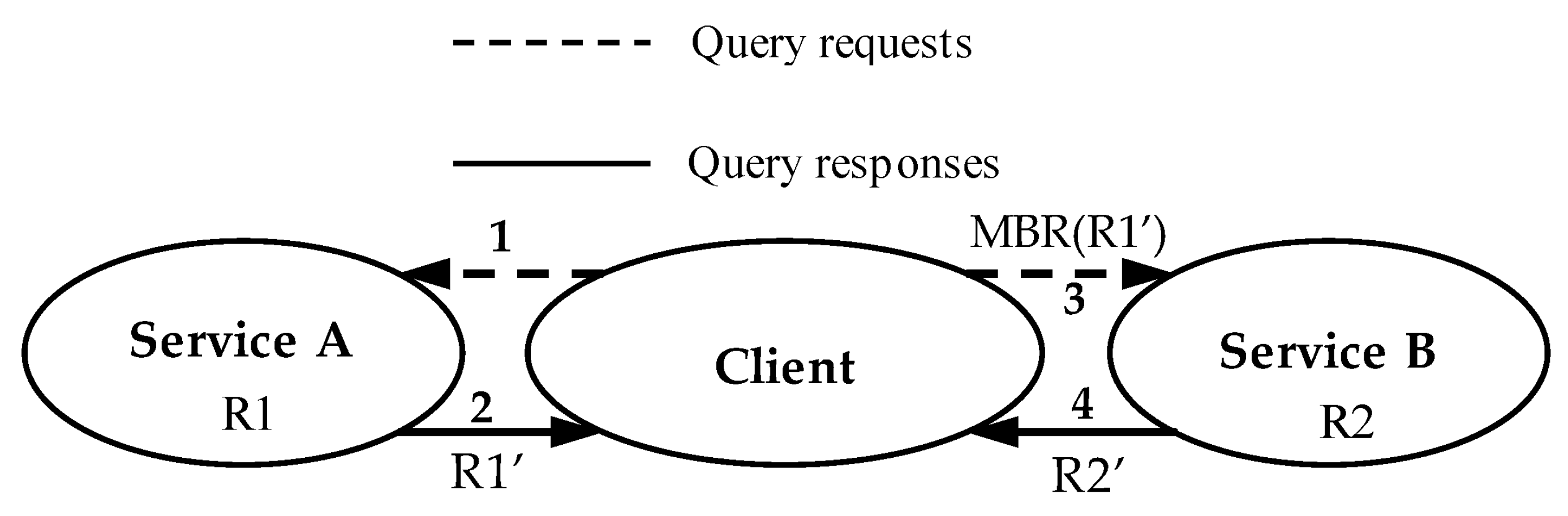
To give an example of this process, we take the spatial semi-join. Suppose that R1 and R2 are two spatial datasets to be joined in a spatial DBMS, and they are deployed on Site A and Site B. To obtain the join result on Site A, a spatial semi-join can expressed as follows [24]: (1) Send MBR(R1) to Site B, where MBR(R1) is the maximum boundary rectangles of the objects in R1. (2) Join MBR(R1) with R2, and obtain the qualified objects in R2, which is denoted as R2′. (3) Send R2′ to Site A, and perform a refinement to obtain the final solution. Comparatively, a spatial join of two WFSs is quite different because the join result should be generated on the client side. Assuming that R1 and R2 are provided by Service A and Service B, respectively, as shown in Figure 1, one approach to perform this spatial semi-join can be described as follows: (1) The client sends the query expression to Service A. (2) Service A sends spatial objects in R1 (denoted by R1′) that satisfy the query condition to the client. (3) The client sends the approximate representation of R1′, MBR(R1′), to Service B. (4) A spatial join of R1′ and R2 is performed on Site B, the candidate objects of R2 are sent to the client, denoted as R2′, and the refinement is performed at the client site.
With the above steps, some objects of R2 would be pruned away, thus reducing the transmission cost. Here, this approach is denoted as Semi_join(R1, R2), and placing R1 first means that the spatial objects on Service A are retrieved first. Obviously, the query can start from Service B and prune away spatial objects of R1, denoted as Semi_join(R2, R1), similarly. In fact, a spatial semi-join is not always effective because in some situations, it cannot prune away enough non-candidate objects of the join result to enhance the performance, and sometimes, it is better to directly retrieve all of the objects from Service A and B, denoted as Direct_join(R1, R2). Let and be the average data sizes of the spatial objects in R1 and R2, let mbr be the data size of a minimum boundary rectangle (MBR), and let N1 and N2 be the numbers of features in R1 and R2; then, the transmission cost of Direct_join(R1, R2) is estimated as × N1 + × N2. Because an MBR can be represented as its left-top and right-bottom vertexes, mbr is set to 2 here. Similarly, the data size of a spatial object is measured as the number of vertexes that it is composed of. Assuming that in Figure 1 the number of objects in R2′ is N2′, then the total transmission cost of Semi_join(R1, R2) can be estimated as × N1 + × N2′ + mbr × N1. Thus, Semi_join(R1, R2) is effective in reducing the transmission cost only if × N2′ + mbr × N1 < × N2. Here, a brief introduction about whether spatial semi-join should be used or not is presented, and a more detailed discussion can be found in [17,18].
In [18], an index called the filtering rate is proposed to estimate to what degree a spatial semi-join can prune away non-candidate objects. Assuming that Semi_join(R1, R2) is performed as in Figure 1, the number of filtered objects will be N2−N2′, and the filtering rate can be expressed as in Equation (1).
Correspondingly, if Semi_join(R2, R1) is performed, then . Because we are inclined to choose the method that can prune away more non-candidate objects, the practical filtering rate can be defined as in Equation (2).
In fact, with regard to N1′ and N2′ beforehand, their approximate values are estimated in the sense of probabilities. Assuming that the spatial objects in N1 and N2 were evenly distributed, the number of intersecting pairs P between the MBRs of R1 objects and those of R2 objects can be estimated by the following equation [25,26]:
where , , , and are the normalized average widths and heights of spatial objects in R1 and R2, respectively, which can be calculated by the sampling method. N1′ and N2′ can be estimated as min(N1, P) and min(N2, P), respectively.
For a spatial join query in which both joined datasets have a large number of spatial objects, simply performing Semi_join(R1, R2) or Semi_join(R2, R1) cannot accelerate the query. In most cases, spatial objects in a dataset are not uniformly distributed; there are sometimes many objects over an area and only a few in the others. If there exists such skewness in a spatial distribution of the two joined datasets, then a partitioning-based strategy will be of great help in reducing the transmission cost. Its basic idea is to partition the whole query area into a certain number of sub-areas, and then, for each sub-area i, to choose the approach with the least cost, thus the whole cost is decreased. The combination of the spatial semi-join and the area partitioning-based method makes this approach sensitive to the skewness in the spatial distribution of two datasets in the sub-areas, and therefore, it is effective even when there is no spatial skewness in the spatial distribution of the joined datasets, as viewed from the whole query area.
For processing the MSJs, perhaps a straightforward approach is to perform binary joins in a certain order, with the aforementioned method used to prune away the non-candidate objects. In fact, similar to processing the MSJs in spatial DBMSs, the ordering of those binary joins can greatly affect the performance. Furthermore, the orderings for the MSJs of WFSs could be more important because it would affect not only the transmission cost but also the cost of encoding spatial objects into GML documents and rebuilding them by parsing the GML documents. In general, the problem of choosing the best order is NP-complete [27]. Some heuristic methods have been proposed for choosing optimal order, such as [28]. In this paper, we use the filtering rate as an indicator for determining which binary join should be performed earlier when searching for a good execution plan.
3. The Optimization Algorithm for a Multi-Way Spatial Join of WFSs
As discussed above, MSJ processing is composed of two elements: processing binary spatial joins and searching for an optimal or sub-optimal execution plan for the whole query, i.e., the ordering of cascading binary spatial joins. In this section, the basic framework for processing binary spatial joins of WFSs is presented by combining the spatial semi-join and partitioning-based methods. Furthermore, we study the properties of the query graph, and we propose a heuristic method that quickly determines good plans by using the filtering rate as an indicator.
3.1. Optimizing Binary Spatial Join of Web Feature Services
As mentioned in Section 2.3, due to the inaccessibility of the spatial indices on WFS servers when processing the spatial joins of WFSs, in this research, the basic idea of the spatial semi-join is combined with partitioning-based methods to prune away non-candidate objects. Generally, there are two types of partitioning methods, i.e., regular grid partitioning and recursive partitioning. Regular grid partitioning partitions the query area into M × N regular cells, while each cell contains spatial objects that fall into its extent. Another kind of partitioning method is recursive partitioning. KD-tree partitioning [29] and quadtree partitioning are two recursive partitioning methods. These methods successively partition the entire query area into sub-areas. If in any of these sub-areas the number of spatial objects in either of the datasets is no more than a threshold T, then that sub-area is stored and no further subdivision is necessary.
Although there are many partitioning methods, for simplicity, we introduce a hybrid method of regular grid partitioning and the spatial semi-join to exemplify the use of this type of method for processing binary spatial join of two WFSs. It should be noted that the number of objects contained in the query area or crossing the boundary, i.e., N1 and N2, are not known at the client side at the beginning, and they are retrieved from the corresponding server by using a “GetFeature” request with the parameter “resultType” being set to “hits,” as introduced in Section 2.1. In the beginning, for each server the client sends a “GetFeature” request to obtain N1 and N2. If both N1 and N2 are far larger than the preset threshold T, the query area is partitioned into M × N regular sub-areas. Let MN = max(N1,N2)/T; it is partitioned in such a way that H/W ≈ N/M and M × N ≈ MN, where W and H are the width and height of the query area respectively. Then, the client sends requests to the two servers to obtain N1i and N2i, i = 1, 2, …, M × N. Similar to the definitions of N1 and N2, N1i and N2i are the numbers of R1 objects and R2 objects contained in the ith sub-area or crossing its boundary. For those sub-areas with a dense distribution of spatial objects of both datasets, i.e., both N1i and N2i are far larger than the threshold T, a further partitioning could be necessary and performed according to the above method. Different from the recursive partitioning method, the partitioning can be limited to no more than two stages. Figure 2 exemplifies the two-stage partitioning. After the partitioning process, for each sub-area, the filtering rate FRi is calculated with Equation (4) [18].
where is the estimated number of candidate objects in the dataset R1 if Semi_join(R2, R1)i is performed for the ith sub-area. Vice versa, is the estimated number of candidate objects in the dataset R2 if Semi_join (R1, R2)i is performed for the ith sub-area. These two quantities are estimated with the selectivity estimation method introduced in [25]. Obviously, if is close to zero, then the spatial semi-join is not suitable for this sub-area, Direct_join (R1, R2)i is chosen instead, and is set to zero. The total filtering rate of the entire spatial join can be expressed as Equation (5).
Two issues should be accounted for in the execution process. One issue is to attempt to reduce the unnecessary requests to the servers as it may increase the execution cost. The other issue is to avoid some objects being repetitively downloaded from WFS servers. Therefore, the homogeneous areas (those to be processed by the same method) are merged into a larger area, and as a result, the times for the interactions between the client and servers will decrease to minimize the time cost. As shown in Figure 2, the sub-areas are classified into three groups according to their execution methods: (a) Semi_join(R2, R1)i, depicted with black cells; (b) Semi_join(R1, R2)i, depicted with white cells; and (c) Direct_join(R1, R2)i, depicted with diagonal cells. Our processing strategy can be expressed in the following three steps:
- (1)
- Merge the white and diagonal sub-areas into a larger area, and send its boundary to Server A to download R1 objects contained in or crossing this boundary. Merge the black and diagonal sub-areas into a larger area, and send its boundary to Server B to download R2 objects contained in or crossing this boundary.
- (2)
- For the white sub-areas, a spatial semi-join is performed on Server B, and the candidate objects of the dataset R2 are sent to the client. For the black sub-areas, a spatial semi-join is performed on Server A and the candidate objects of the dataset R1 are sent to the client.
- (3)
- The immediate datasets are refined on the client side to obtain the final solutions of the spatial join.
The above processing strategy works on the assumption that both datasets must be transmitted to the client. Another situation is that one of the two joined datasets has been transmitted to the client, and only the non-candidate objects of the other dataset must be pruned away. Assuming that there is a three-way join R1⋈R2⋈R3, after R1⋈R2 has been completed, R2′ is cached in the client site, and the remaining R2′⋈R3 can be performed as follows: Merge sub-areas with dense distribution of R2′ objects into a larger area, and download the objects of R3 in this area. Merge the other sub-areas, and send the maximum boundary rectangles (MBRs) of the R2′ objects in the merged area to the server of R3; after performing a spatial semi-join, the qualified objects of R3 dataset in this area are sent to the client. The set of all of the downloaded R3 objects is denoted by R3′. Last, the objects in R1′, R2′ and R3′ can be tested to find the solutions to the join R1⋈R2⋈R3 with conventional algorithms.
3.2. Optimizing the Multi-Way Spatial Joins of Web Feature Services
Different from binary spatial join processing, the main concern of multi-way join optimization is to search for an optimal or sub-optimal execution plan that has a certain ordering of binary joins, to prune away as many non-candidate objects as possible. As in distributed spatial DBMSs, information about the datasets, such as spatial indexes, is much cheaper to access, and therefore an optimal plan is easier to achieve by employing some complicated optimization methods. When processing MSJs on a client computer, such information is impossible or costly to achieve. Therefore, methods such as dynamic programming are not feasible in processing queries of WFSs, and we must use a more straightforward and cheaper method.
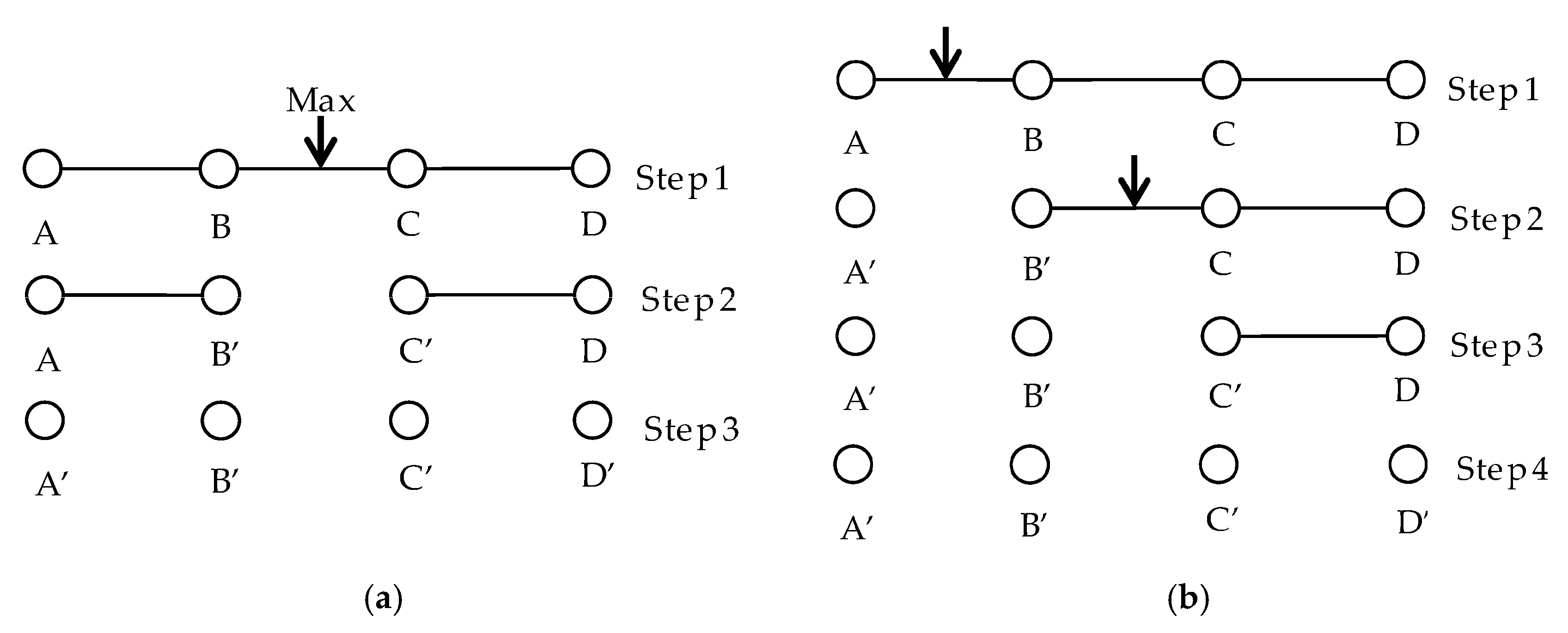
Perhaps the most important task here is to determine what type of joins should be performed earlier. Consider the join graph shown in Figure 3: there are four datasets, A, B, C and D, and three join operations between the adjacent two datasets. If the join of datasets B and C has a high filtering rate, as shown in Figure 3a, let and be the distinct objects in the solution of B⋈C. Then, it can be obtained that << and/or <<, where , , and are the numbers of objects of , , and respectively. If <<, then the transmission cost of the following join⋈A will be greatly reduced in consequence. In contrast, if the execution plan in Figure 3b is chosen, then A⋈B is performed first, and many objects in A and B would be downloaded to the client site; however, most of them are not qualified for the join A⋈B⋈C, which means that they cannot be present in the solutions of the whole join. Therefore, it is better to perform a join that has a higher filtering rate earlier. On the other hand, for a given binary join, if both datasets have far fewer features than the other datasets in the adjacent joins, such a join can also be performed early because its execution would likely not decrease the performance of the whole query.
Based on the above ideas, our optimization algorithm mainly consists of three steps, as follows:
- (1)
- Estimate the filtering rates for all of the binary joins in the query graph with Equation (2).
- (2)
- Perform the join with the highest priority (usually determined by the filtering rate). After that, recalculate the filtering rate of the other binary joins with respect to the above two joined datasets, if necessary.
- (3)
- Repeatedly perform step (2) until all of the candidate objects of the related datasets have been downloaded to the client site.
The pseudo-code in Algorithm 1 shows a brief idea of how a multi-way spatial join is processed.
| Algorithm 1: Processing multi-way spatial joins |
| Multiway-SpatialJoin(Datasets){ Foreach (Relation(i, j) in RelationSets) { /*Compute filtering rates for every binary join */ S(i, j)=ComputeFilteringRate (Datasets[i], Datasets[j]); } While (RelationSets ≠∅){ /*Stop if RelationSets is empty*/ Find the binary join with them maximum filtering rate S(n, m) or the Relation(n, m) that both datasets have a very small number of features; SpatialJoin(Datasets[n], Datasets[m]); /*Join Datasets[n] and Datasets[m]*/ Update(Datasets[n], Datasets[m]); /* Substitute Datasets[n] and Datasets[m] with the immediate solution of the previous join*/ Remove( Relation(n, m) ); /*Remove Relation(n, m) from RelationSets */ Update the filtering rates of the other joins that Datasets[n] and Datasets[m] participate in; } } |
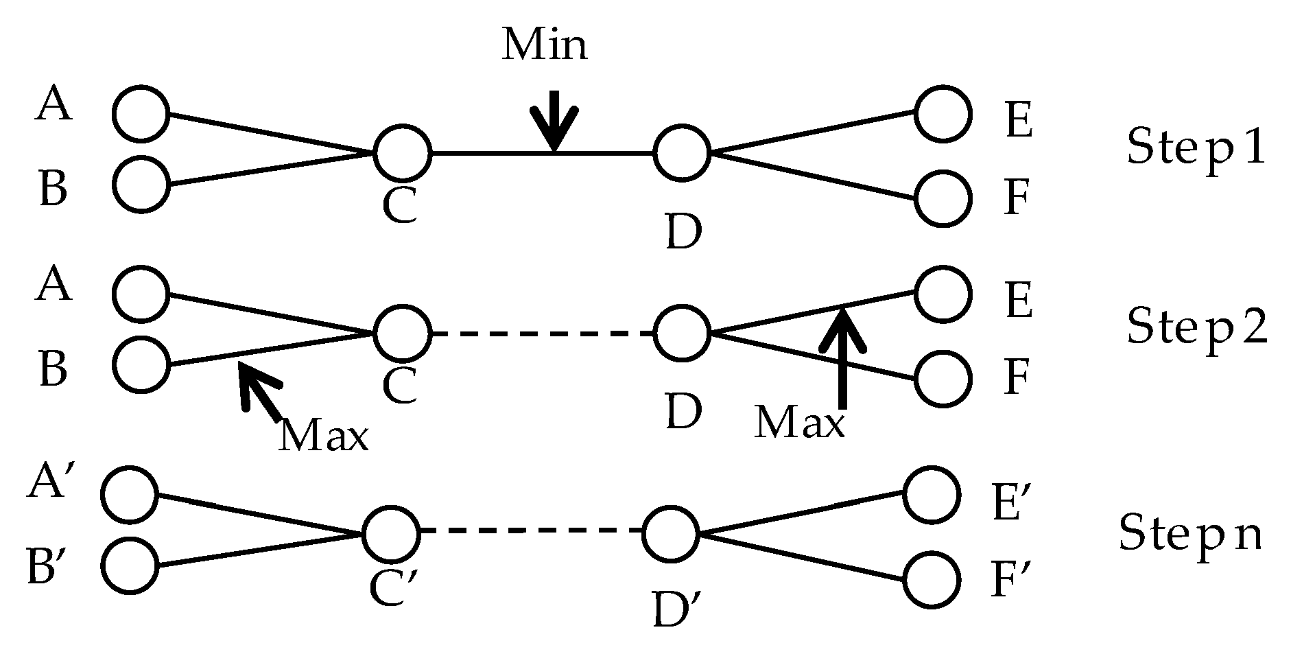
The above method performs binary joins in a sequential order. When there are adequate computational resources, some complex queries can be broken down into a certain number of parts that can be performed in parallel to speed up the whole join. Assuming in Figure 4 C⋈D a very low filtering rate, performing it ahead is no help for pruning away non-candidate objects of the adjacent joins, such as D⋈E and D⋈F. The query graph can thus be broken down into two parts, A⋈C⋈B and E⋈D⋈F. Moreover, they are subject to the abovementioned steps. Because parallel processing is not our concern in this paper, we do not experiment with the method shown in Figure 4.
4. Experiment Analysis
To verify the feasibility of our optimization methods, a mock-up WFS server program and a client program were developed with Visual Studio 2008 C# and ArcGIS Engine9.3. The server program is an ASP.Net web service which handles the query requests. And in the background, query processing is performed by calling the programming interfaces provided by ArcGIS Engine9.3. On each server computer, the server program is deployed to an IIS7.0 server. The client program is a Windows application, which provides the following functionalities: (1) parse response documents, especially the spatial objects represented in XML format, which are parsed and stored into ESRI shape files, and (2) perform binary spatial joins and/or multi-way spatial joins by using our strategies, with the support of ArcGIS Engine SDK. With these programs, experiments in three stages are performed. The focus of the first stage is to testify the binary spatial join strategy introduced in Section 3.1, and that of the second stage is to determine whether our method for processing MSJ is feasible or not. The last stage aims at simulating how the proposed method behaves when the servers and the clients are connected with different connection speeds.
4.1. Test of Binary Spatial Join
In this experiment, three computers were used to act as Server A, Server B and the client. Server A and Server B were equipped with Intel(R) Xeon(CPU) [email protected] GHz, 4G RAM. The client was equipped with Pentium(R) Dual-Core CPU [email protected] GHz. All the computers used Win7 Sp1 as their operating systems. Two datasets of 2015 TIGER/Line [30] provided by the United States Census Bureau, called tl_2015_us_uac10 and tl_2015_us_place, were chosen as joined datasets. They were deployed at Server A and Server B, respectively. Three processing strategies were implemented and deployed on the client site: (1) to directly download and join all of the objects of the datasets in the query area, which was used as the performance baseline, abbreviated as “DDJ” in the following; (2) to process the binary spatial joins with regular grid partitioning, as described in Section 3.1; and (3) to process the binary spatial joins with recursive partitioning.
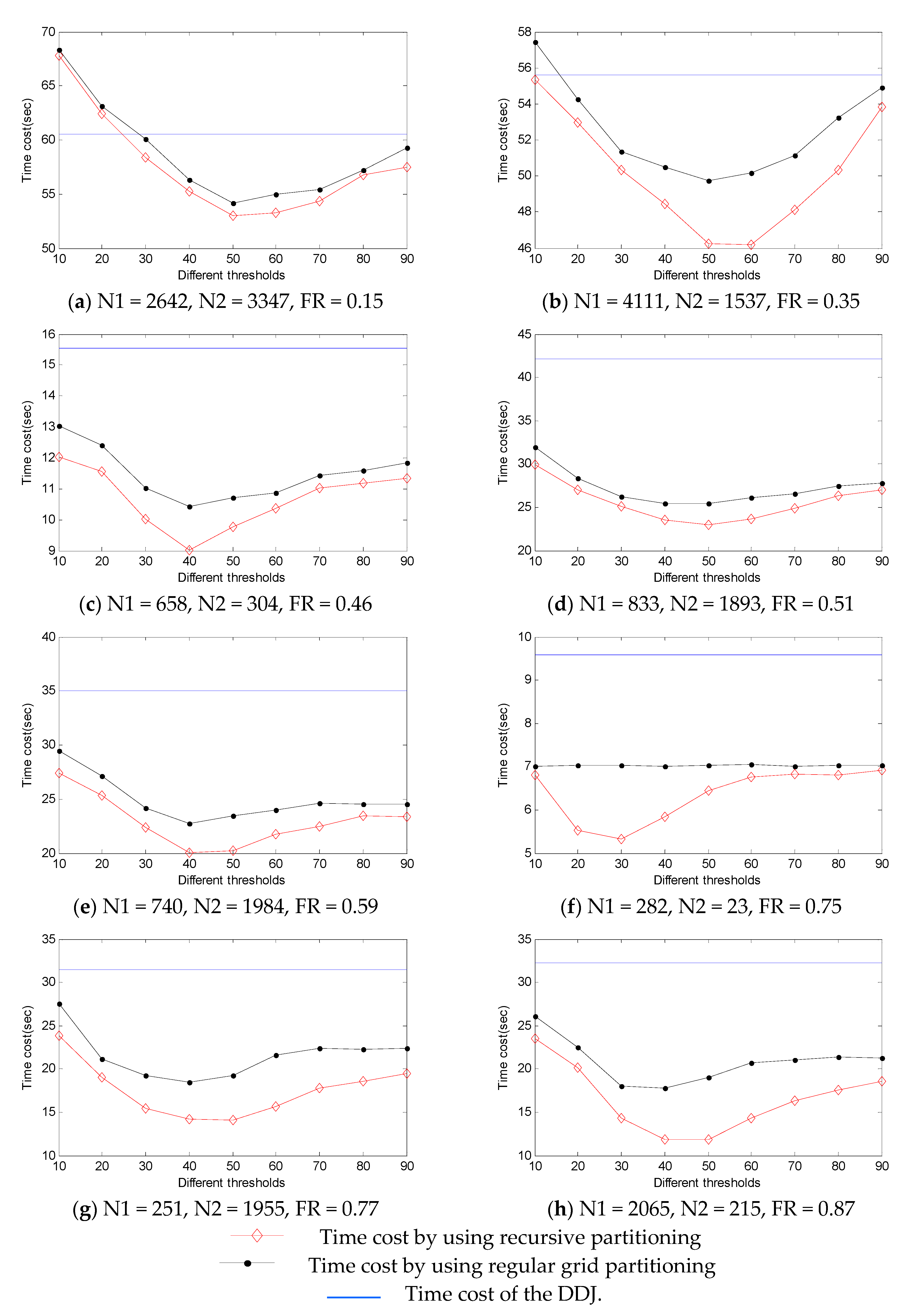
In our experiments, eight testing areas in the extents of the spatial datasets were selected as areas to be tested, and for each area a certain number of spatial joins were performed with the above three strategies using a randomly selected query window of 300 km × 300 km. In Section 3.1, it has been stated that a threshold T is used to determine whether an area should be partitioned or not. Here, a set of thresholds (T = 10, 20, 30, 40, 50, 60, 70, 80, 90) is used, as shown in Figure 5. For each query window, a spatial join was performed with the three strategies using all thresholds; in other words, it is performed 9 + 9 + 1 = 19 times. Figure 5 shows the execution time required when different thresholds are used, and the object numbers of both datasets and the estimated FRs are also provided.
As shown in Figure 5, comparatively, recursive partitioning outperforms regular grid partitioning. However, the effectiveness of the optimization methods is affected by many factors, such as the geometric complexity of the spatial objects, their spatial distribution and the partitioning threshold T. When the spatial objects are evenly distributed in two-dimensional space, the filter rate is relatively low and there is not much difference in performance between the methods. Figure 5a illustrates this case. While the spatial objects are not evenly distributed, and the filter rate is relatively high, such as the join shown in Figure 5e, recursive partitioning strikingly outperforms regular grid partitioning. The performance is also greatly affected by the partitioning threshold T. If T is too large, then the partitioning method is not sensitive to the spatial skewness, and the performance could hardly be improved. In contract, if T is too small, then unnecessary partitioning will incur too much overhead. The best T for a certain join is determined by the abovementioned factors, and in fact it is impossible to determine it for a certain join. According to our experience, it ranges from approximately 30 to 60.
To further validate our hypothesis, another 92 windows are used to conduct the abovementioned experiment, except that only three partitioning thresholds (T = 30, 50, 100) are used here. Thus far, the experimental result of 100 windows is collected. According to the number of objects involved in a spatial join (denoted as NS), the 100 windows were classified into seven groups, listed as follows: NS∈[1, 100], six windows; NS∈[101, 300], 21 windows; NS∈[301, 500], 25 windows; NS∈[501, 1000], 18 windows; NS∈[1001, 2000], 16 windows; NS∈[2001, 3000], eight windows; and NS∈[3001, 6000], six windows. Let X be the ratio of the execution time of DDJ to that of the optimization method; then, the effectiveness of the proposed method can be classified as follows: X ≥ 1.5, notable performance improvement; 1.5 > X > 1.0, slight performance improvement; and X ≤ 1.0, futile. Table 2 and Table 3 show that the performance improved by using the two partitioning methods.
As shown in Table 2 and Table 3, the optimization method is futile for approximately 20−23 windows. Still we find that more windows are proven to achieve a notable improvement in performance when T is set to 50. When T = 50 and recursive partitioning is used, all six joins of NS∈[1, 100] cannot be improved, which accounts for 27.3% of the futile tests. When NS∈[1, 500], 13 joins cannot be improved, which accounts for 59.1% of the futile tests. This finding arises because there is no room for improvement in performance when there are only a few objects to be joined. When NS∈[101, 2000], the notable improved joins account for 84.3% of all of the 70 joins that are notably improved; when NS∈[2000, 6000], 11 of 14 joins are notably improved. It can be concluded that the optimization method is more effective with the increasing number of spatial objects involved. Nevertheless, there could be some reasons that recursive partitioning outperforms regular grid partitioning slightly based on this experimental result: (1) The query areas chosen are square, while regular grid partitioning is expected to work better when the query areas are rectangular; (2) A query area is partitioned into M × N ≈ MN sub-areas in the first stage of regular grid partitioning, and perhaps, M × N ≈ MN/α should be used instead to avoid excessing partitioning, where α is a parameter that is set to a number larger than 1, e.g., 1.5 or 2.
To sum up, the combination of spatial semi-join and area partitioning will incur some additional overheads to search for suitable methods for the sub-areas. If there are adequate non-candidate objects being pruned away, this type of method will improve the performance. Moreover, the proposed strategy has been designed to avoid over-partitioning in order to prevent serious performance decrease. Comparatively speaking, the DDJ method does not attempt to prune away non-candidate objects, and it does not require the cost on the above procedures, but it is the best choice only for the spatial joins that have most of the objects in the query areas present in the final results.
4.2. Test of Multi-Way Spatial Join
In the second stage, three methods are compared in terms of the time cost: (1) the optimization method, denoted as M1; (2) the method that performing binary joins in the initial order, denoted as M2; and (3) the DDJ method, denoted as M3 and used as a performance baseline. Our experiments of multi-way spatial joins involve five datasets from Census 2015 TIGER/Line Shapefiles. Their spatial extent ranges from a longitude of −124.5° to −67.9° and from a latitude of 23.9° to 49.1°. Table 4 gives a brief description of the spatial datasets.
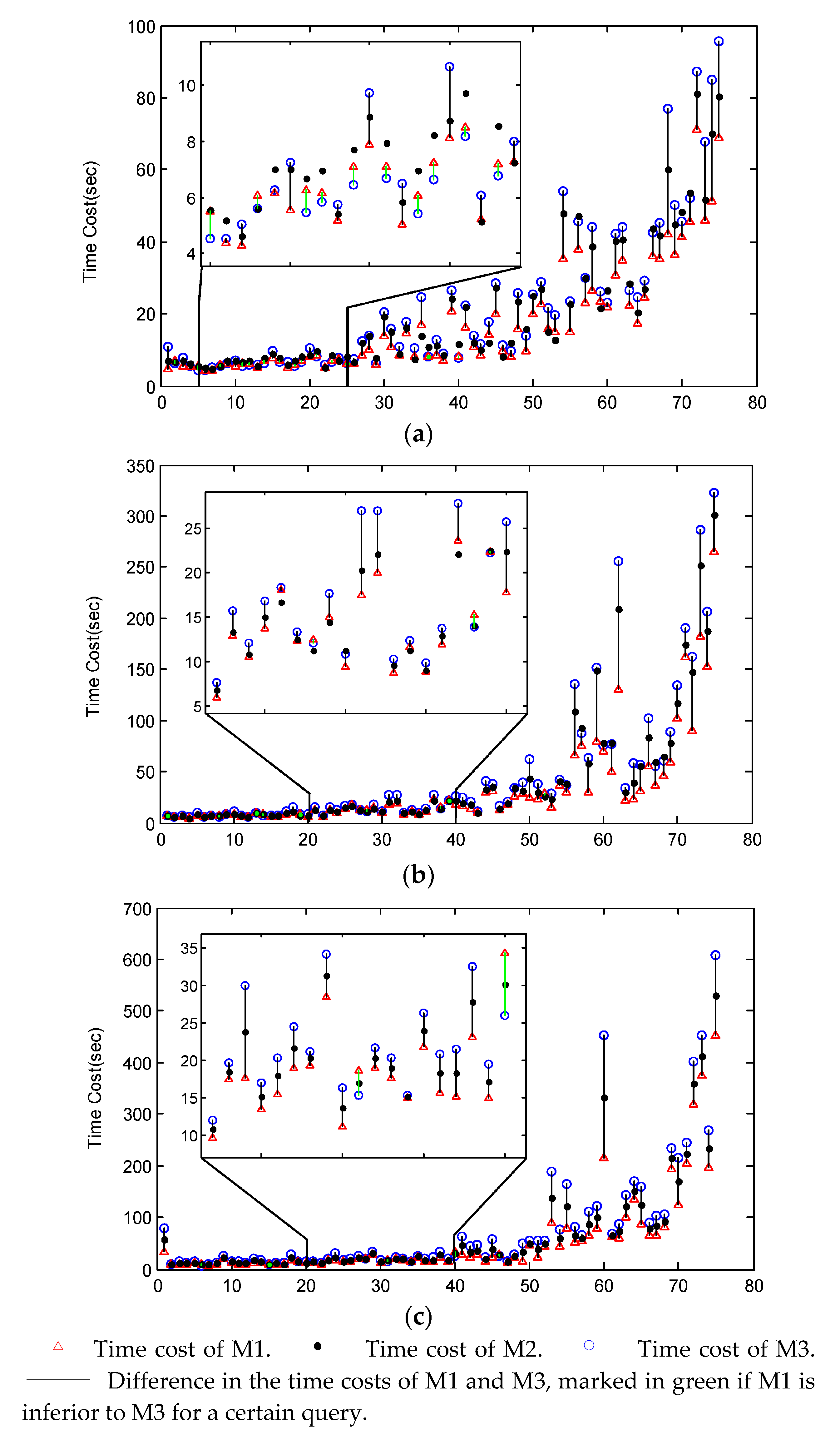
With these datasets, three types of spatial joins, [primary roads] ⋈ [uac10] ⋈ [place], [primary roads] ⋈ [uac10] ⋈ [place] ⋈ [rails], and [primary roads] ⋈ [uac10] ⋈ [place] ⋈ [rails] ⋈ [school], are performed in our experiment. As spatial intersect is the most commonly used spatial predicate, we chose it as the spatial predicate in our experiments. The spatial extent of all of the datasets is uniformly partitioned into 8 × 18 grids, and those with a relatively intensive spatial distribution of spatial objects were selected to perform our experiments. The size of the query window is 300 km × 300 km. For every multi-way spatial join, the number of spatial objects in its query area, the number of tuples in its solution, and the execution times of the three methods are recorded. In our experiments, 75 grids are used as our experimental areas, and the time costs of three types of spatial joins are shown in Figure 6. In Figure 6a–c, the vertical axis represents the time cost, and the horizontal axis shows the identity numbers of the 75 grids, which are sorted in ascending order according to the number of objects of the joined datasets in the query area. Moreover, the time costs of the three methods are compared in Table 5.
In the magnification window of Figure 6a, for 10 of 20 queries, the time cost of M1 is slightly higher than that of M3, mainly for the reason that there are only a few spatial objects in the query windows, ranging from approximately 100 to 200 in this case. Comparatively, for the queries shown in Figure 6b,c, the number of the involved objects ranges from approximately 700 to 1400. Because searching for the optimal execution plan incurs some additional costs caused by the pre-processing procedures, such as computing the spatial distributions of the objects, when there are not enough objects to be filtered, M3 will perform slightly better than M1. However, when the number of datasets increases, M1 is obviously superior to M3. The experimental results show that in most cases our optimization method can reduce the non-candidate objects effectively, which will minimize the (CPU+I/O) time cost and the transmission cost at the same time, to compensate for the time cost of interactions between the servers and the client, thus enhancing the performance in processing multi-way spatial joins. Moreover, from Figure 6 and Table 5, it is clear that M2 is superior to M3, but overall, M1 is the best method. When the initial order is the optimal approach, M2 is obviously the best choice because it does not have to search for the optimal order.
4.3. Test with Different Connection Speeds
The above experiments are conducted on a LAN with a transfer speed up to 100 Mbps. However, in a WAN scenario, a client may be connected to the servers with different bandwidths and latencies, so it is difficult to ensure such a high sustained data transfer rate. To examine the performance of the proposed method in that scenario, we conducted an experiment under the circumstances that the servers and the client are connected with different connection speeds, as shown in Table 6 and Table 7. The speeds were limited by changing the configuration of the router. In this experiment, twelve 300 km × 300 km query areas are randomly selected to perform the four-way spatial join introduced in Section 4.2, under the circumstances that the servers and the client are connected with different connection speeds. The number of the involved objects in a query area ranges from approximately 640 to 3800. Table 6 shows the time costs of the optimization method and the DDJ method. Derived from Table 6, Table 7 shows the ratios of the time costs of M1 versus M2. From Table 6 and Table 7, the time costs of both M1 and M3 increase as the connection speed decreases. Meanwhile M3 is relatively susceptible to the connection speed, and M1 outperforms M3 to a greater or lesser degree. This experimental result implies that the optimization method is more practical when the servers and the clients are connected with a low transfer speed.
5. Discussion
Processing a multi-way spatial join is very complicated. In distributed spatial database management systems (DBMSs), although the performance of this type of join can be improved by some faster algorithms and optimization techniques, there are still very few existing studies that address multi-way spatial join (MSJ) of Web Feature Services (WFSs). The optimization of MSJ of WFSs introduced in this paper involves two issues: (1) to search for methods of pruning away non-candidate objects for binary spatial joins and (2) to search for an optimal or sub-optimal order of binary joins decomposed from a complicated join. Our approaches for processing binary spatial join are developed by combining spatial semi-join and partitioning-based methods. Additionally, the filtering rate is utilized to search for the execution order of the binary spatial joins that are decomposed from a complex query.
The estimated filtering rate means the potential to improve the performance by using spatial semi-join. In practice, some types of geographical phenomena are strongly related in spatial distributions, e.g., there are always some grocery stores near an elementary school in some countries. Because the probability that a grocery store is located near an elementary school is high, a query “find all the elementary schools within 50 m of a grocery store” has very little potential to prune away non-candidate objects by spatial semi-join. In other words, the spatial semi-join is largely ineffective for those strongly related datasets. However, in many cases, spatial objects are not uniformly distributed and spatially strongly related; therefore, adequate filtering rates are expected to be achieved and the spatial semi-join can be used as an effective method to prune away non-candidate objects for MSJ of WFSs. The accuracy of estimating the filtering rate is heavily affected by the complexity of the geometric representation of spatial objects. Our method for estimating the filtering rate is deduced from the selectivity estimation of the spatial joins. Most of the current methods on selectivity estimation determine the selectivity based on the probability of a spatial intersection of the maximum boundary rectangles of the spatial objects. Errors are impossible to avoid in estimating the filtering rate, and sometimes, the estimating errors are unacceptable. Statistically, these methods do work well for polygon objects but sometimes not for polyline objects.
Another factor that affects the performance is the selection of the partitioning methods. For datasets with a uniform spatial distribution, there is very little difference between the two partitioning methods in terms of the performance. For those datasets that have a skewed spatial distribution, a query area is divided into fewer sub-areas by recursive partitioning than regular grid partitioning, and thus, in this case, less interaction between the client and the servers is required to find the spatial distributions of the joined datasets by using recursive partitioning. The partitioning threshold T is also an important performance factor; in this paper, it is recommended to be set at approximately 50. The number of spatial objects in the two joined datasets is also a factor in the potential for performance improvement. When there is only a small number of objects, partitioning does not occur in the query processing, and it does not help to improve performance. The combination of a partitioning method and spatial semi-join is more effective when more spatial objects in two datasets are joined.
In this paper we have developed a method for determining the order of binary spatial joins decomposed from a complex query. This method attempts to perform the binary joins with high filtering rates in the beginning, to reduce the inputs of the subsequent binary joins. Because generating the best execution plans could incur too expensive an overhead, our method aims to determine sub-optimal plans. When compared with the simple methods (M2 and M3 in Section 4.2), the disadvantages of the proposed method can be concluded as follows. First, more requests are required to determine the distribution of objects, which may bring up some additional pressures on the servers. Second, in some cases, such as when the true filtering rates are too low, or the original order is actually the best order, it is fruitless to search for an optimal execution plan. Third, as transmission cost is not dominant in a high speed network, this method is less effective in this situation. Fourth, the client program needs to be elaborately designed. However, with the filtering effect of the spatial predicates, when more datasets are involved in an MSJ, there is more potential to improve the performance by pruning away non-candidate objects. As in most cases, less objects need to be encoded into GML format at the server side and decoded at the client side; computational overheads are subsequently reduced on both sides, and the response time of the client will be shortened. In summary, our experimental result shows that the optimization method outperforms the other two methods in processing multi-way spatial joins.
Acknowledgments
This research was supported by the National Natural Science Foundation of China under Grant No. 41261088, the ‘Ba Gui Scholars’ program of the provincial government of Guangxi, and the Graduate innovation program of Guangxi under Grant No. 002504216008.
Author Contributions
Guiwen Lan proposed the method and design the experimental plan, wrote the manuscript and modified it; Qiang Zhang designed and implemented the computer programs for the experiments, and finished the experimental analysis; Tong Li and Zhao Yang prepared the spatial datasets for the experiments.
Conflicts of Interest
The authors declare that they have no conflict of interest.
References
- Farruque, N.; Osborn, W. Efficient distributed spatial semijoins and their application in multiple-site queries. In Proceedings of the 28th IEEE International Conference on Advanced Information Networking and Applications (AINA 2014), Victoria, BC, Canada, 13–16 May 2014; pp. 1089–1096. [Google Scholar]
- Open Geospatial Consortium Inc. OGC®Web Feature Service Implementation Specification. 2005. Available online: http://portal.opengeospatial.org/files/?artifact_id=8339 (accessed on 10 April 2016).
- Open Geospatial Consortium Inc. OGC®OpenGIS Web Feature Service 2.0 Interface Standard. 2010. Available online: http://portal.opengeospatial.org/files/?artifact_id=39967 (accessed on 10 April 2016).
- Gong, J.; Jia, W.; Chen, Y.; Xie, J. Development from platform GIS to cross-platform interoperable GIS. Geomat. Inf. Sci. Wuhan Univ. 2004, 29, 985–989. [Google Scholar]
- Xie, J.; Gong, J. Application of wfs in land and resources multilevel databases remote synchronization. Proc. SPIE 2005. [Google Scholar] [CrossRef]
- Zheng, W.F.; Wang, X.B.; Yin, A.T.; Kan, A.K.; Li, H.R. Application of web feature service-based data share to earthquake disaster reduction. J. Nat. Disasters 2008, 17, 1–5. [Google Scholar]
- Zhang, C.; Zhao, T.; Li, W. Towards improving query performance of web feature services (WFS) for disaster response. ISPRS Int. J. Geo-Inf. 2013, 2, 67–81. [Google Scholar] [CrossRef]
- Qi, M.Y. Research on Logistics Oriented Spatial Information Service and Its Key Techniques Issues; Institute of Remote Sensing Applications, Chinese Academy of Sciences: Beijing, China, 2006. [Google Scholar]
- Jia, W.J.; Gong, J.Y.; Li, B. Optimization method of web feature service. Acta Geod. Cartogr. Sin. 2005, 34, 168–174. [Google Scholar]
- Wu, H.; Zhe, L.; Xu, K. Cascading model of geospatial information service integration and its application. Sci. Surv. Mapp. 2010, 35, 212–214. [Google Scholar]
- Bai, Y.; Yang, C. Research on spatial information search engine. J. China Univ. Min. Technol. 2004, 33, 90–94. [Google Scholar]
- Jiang, J.; Yang, C.; Ren, Y. A spatial information crawler for OpenGIS WFS. Proc. SPIE 2008. [Google Scholar] [CrossRef]
- Mamoulis, N.; Papadias, D. Multiway spatial joins. ACM Trans. Database Syst. 2001, 26, 424–475. [Google Scholar] [CrossRef]
- Park, H.-H.; Cho, H.-J.; Chung, C.-W. Heuristic approach for early separated filter and refinement strategy in spatial query optimization. J. Syst. Softw. 2002, 62, 161–179. [Google Scholar] [CrossRef]
- Lu, H.; Shan, M.-C.; Tan, K.-L. Optimization of multi-way join queries for parallel execution. Proceessdings of the 17th International Conference on Very Large Data Bases, Barcelona, Spain, 3–9 September 1991; pp. 549–560. [Google Scholar]
- Lin, X.; Lu, H.X.; Zhang, Q. Graph partition based multi-way spatial joins. In Proceedings of the IEEE International Database Engineering and Applications Symposium (IDEAS’02), Edmonton, AB, Canada, 17–19 July 2002. [Google Scholar] [CrossRef]
- Lan, G.; Huang, Q.; Zhou, X. A spatial join strategy between ogc-compliant web feature services. Geomat. Inf. Sci. Wuhan Univ. 2009, 34, 655–658. [Google Scholar]
- Lan, G.; Wu, C.; Shi, G.; Chen, Q.; Yang, Z. Spatial join optimization among WFSs based on recursive partitioning and filtering rate estimation. Proc. SPIE 2015. [Google Scholar] [CrossRef]
- Lo, M.-L.; Ravishankar, V.C. Spatial hash-joins. In Proceedings of the ACM SIGMOD conference, Montreal, QC, Canada, 4–6 June 1996; pp. 247–258. [Google Scholar]
- Patel, J.M.; DeWitt, D.J. Partition based spatial–merge join. In Proceedings of the ACM SIGMOD conference, Montreal, QC, Canada; 1996; pp. 1–12. [Google Scholar]
- Arge, L.; Procopiuc, O. Scalable sweeping-based spatial join. In Proceedings of the International Conference on Very Large Data Bases, New York, NY, USA, 24–27 August 1998; pp. 324–335. [Google Scholar]
- Jacox, E.H.; Samet, H. Iterative spatial join. ACM Trans. Database Syst. 2003, 28, 230–256. [Google Scholar] [CrossRef]
- Papadias, D.; Mamoulis, N.; Theodoridis, Y. Constraint-based processing of multiway spatial joins. Algorithmica 2014, 30, 188–215. [Google Scholar] [CrossRef]
- Abel, D.J.; Ooi, B.C.; Tan, K.L.; Power, R.; Yu, J.X. Spatial join strategies in distributed spatial dbms. In Proceedings of the 4th International Symposium on Lame Spatial Databases, Portland, OR, USA, 6–9 August 1995; pp. 348–367. [Google Scholar]
- An, N.; Yang, Z.; Sivasubramanium, A. Selectivity estimation for spatial joins. In Proceedings of the 17th International Conference on Data Engineering, Heidelberg, Germany, 2–6 April 2001; pp. 368–375. [Google Scholar]
- Sun, C.; Agrawal, D.; Abbadi, A.E. Selectivity estimation for spatial joins with geometric selections. In Proceedings of the 8th International Conference on Extending Database Technology (EDBT 2002), Prague, Czech Republic, 25–27 March 2002; pp. 609–626. [Google Scholar]
- Karam, O. Optimizing Distributed Spatial Joins; Tulane University: New Orleans, LA, USA, 2001. [Google Scholar]
- Osborn, W.; Zaamout, S. Multiple-site distributed spatial query optimization using spatial semijoins. In Proceedings of the 10th International Baltic Conference on Databases and Information Systems (Baltic DB&IS 2012), Vilnius, Lithuania, 8–11 July 2012. [Google Scholar]
- Zhou, Q.H.; Chen, L.; Jing, N. Distributed spatial join query based on kd-tree recursive partitioning. Comput. Eng. Sci. 2011, 33, 167–172. [Google Scholar]
- U.S. Census Bureau. Census 2015 Tiger/Line Shapefiles. Available online: http://www.census.gov/ (accessed on 20 October 2016).
Figure 1.
Spatial semi-join between two Web Feature Services (WFSs).

Figure 2.
Partitioning and merging the sub-areas with same execution approaches.
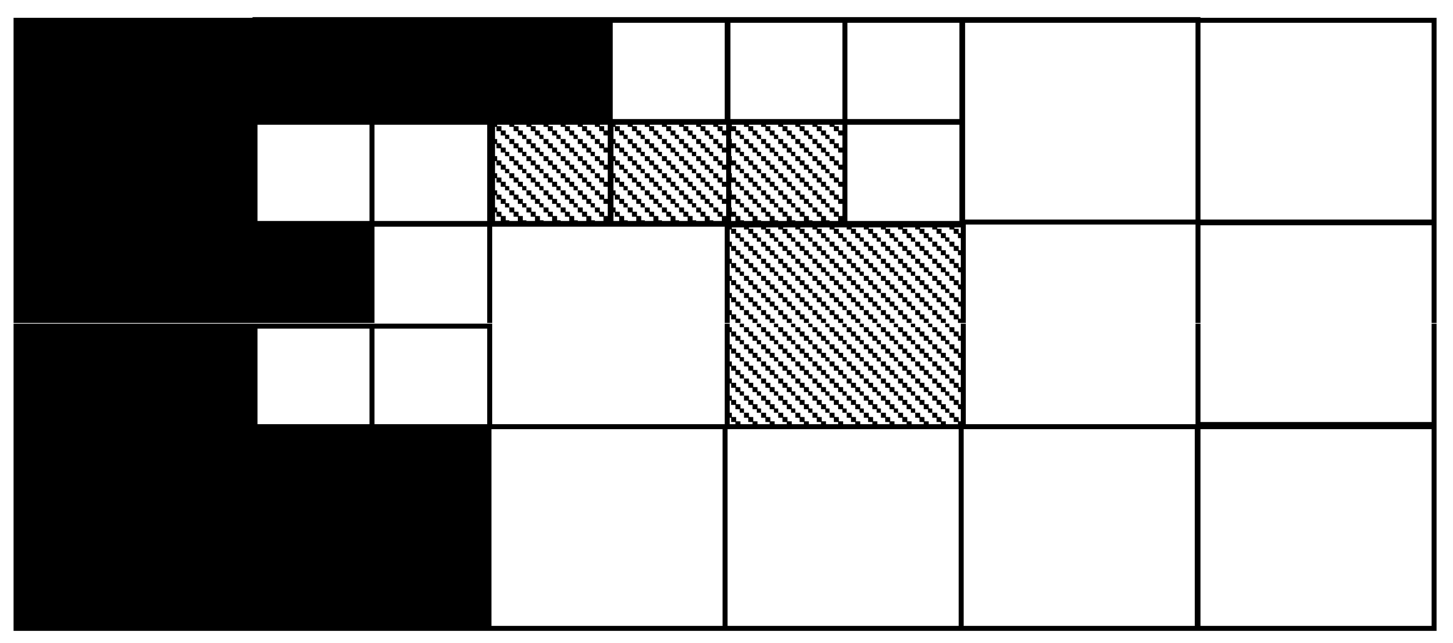
Figure 3.
Two execution plans of a four-way join. (a) Perform the join with maximum filtering rate first; (b) Perform binary joins in order from left to right.
Figure 3.
Two execution plans of a four-way join. (a) Perform the join with maximum filtering rate first; (b) Perform binary joins in order from left to right.

Figure 4.
The query graph is broken down into two parts and the join C⋈D (with the lowest filtering rate) is performed last.
Figure 4.
The query graph is broken down into two parts and the join C⋈D (with the lowest filtering rate) is performed last.

Figure 5.
Comparison of the two partitioning methods in terms of the performance.

Figure 6.
Time costs of the five-way spatial joins by the two methods. (a) Time costs of the three-way spatial joins by the three methods; (b) Time costs of the four-way spatial joins by the three methods; (c) Time costs of the five-way spatial joins by the three methods.
Figure 6.
Time costs of the five-way spatial joins by the two methods. (a) Time costs of the three-way spatial joins by the three methods; (b) Time costs of the four-way spatial joins by the three methods; (c) Time costs of the five-way spatial joins by the three methods.


Table 1.
Time costs of the different steps of ten portions of tl_2015_us_ rails with different data sizes.
Table 1.
Time costs of the different steps of ten portions of tl_2015_us_ rails with different data sizes.
| No. | DS_SHF (MB) | DS_XML (KB) | ENCODE_T (s) | PARSE_T (s) | TRANS_T (s) | TOTAL (s) |
|---|---|---|---|---|---|---|
| 1 | 1 | 2472 | 0.82 | 1.14 | 0.66 | 2.62 |
| 2 | 3 | 7476 | 2.44 | 3.69 | 1.37 | 7.5 |
| 3 | 5 | 12,932 | 4.42 | 6.23 | 2.56 | 13.21 |
| 4 | 7 | 17,835 | 5.95 | 8.76 | 4.08 | 18.79 |
| 5 | 9 | 22,902 | 7.54 | 11.07 | 5.43 | 24.04 |
| 6 | 11 | 28,343 | 9.3 | 13.75 | 6.88 | 29.93 |
| 7 | 13 | 33,749 | 13.08 | 17.79 | 9.1 | 39.97 |
| 8 | 15 | 38,293 | 15.1 | 19.92 | 11.07 | 46.09 |
| 9 | 17 | 44,420 | 17 | 23.75 | 12.32 | 53.07 |
| 10 | 19 | 49,157 | 20.03 | 26.87 | 13.53 | 60.43 |
Table 2.
Performance improvement by using regular grid partitioning.
| T = 30 | T = 50 | T = 100 | Average | |
|---|---|---|---|---|
| X ≥ 1.5 | 45.0% | 60.0% | 42.0% | 49.0% |
| 1.5 > X > 1.0 | 32.0% | 20.0% | 35.0% | 29.0% |
| X ≤ 1.0 | 23.0% | 20.0% | 23.0% | 22.0% |
Table 3.
Performance improvement by using recursive partitioning.
| T = 30 | T = 50 | T = 100 | Average | |
|---|---|---|---|---|
| X ≥ 1.5 | 53.0% | 70.0% | 51.0% | 58.0% |
| 1.5 > X >1.0 | 24.0% | 8.0% | 26.0% | 19.3% |
| X ≤ 1.0 | 23.0% | 22.0% | 23.0% | 22.7% |
Table 4.
The datasets used in our experiments.
| Dataset Name | Geometric Type | Number of Objects | Data Size (kb) |
|---|---|---|---|
| primary roads | polyline | 12,101 | 40,061 |
| uac10 | polygon | 3976 | 108,422 |
| place | polygon | 29,130 | 167,240 |
| rails | polyline | 180,739 | 64,872 |
| school | polygon | 6846 | 171,507 |
Table 5.
Comparison of M1 and M2 with M3.
| Types | Number of Objects | Notably Improved | Slightly Improved | Futile | |||
|---|---|---|---|---|---|---|---|
| M1 | M2 | M1 | M2 | M1 | M2 | ||
| Three-way | [54,1349] | 7 | 3 | 54 | 47 | 14 | 25 |
| Four-way | [196,4131] | 18 | 0 | 48 | 59 | 9 | 16 |
| Five-way | [234,4271] | 20 | 1 | 50 | 69 | 5 | 5 |
Table 6.
Time costs of M1 and M3 under the circumstances of different connection speeds.
| Speed | Unlimited | 4 Mbps | 2 Mbps | 1 Mbps | 0.5 Mbps | |||||
|---|---|---|---|---|---|---|---|---|---|---|
| NO. | M1 | M3 | M1 | M3 | M1 | M3 | M1 | M3 | M1 | M3 |
| 1 | 13.02 | 14.86 | 13.39 | 15.56 | 13.37 | 17.42 | 14.23 | 20.84 | 19.72 | 31.37 |
| 1 | 17.12 | 22.12 | 19.86 | 28.52 | 24.39 | 36.89 | 32.37 | 48.74 | 45.98 | 71.24 |
| 2 | 22.45 | 31.32 | 29.07 | 44.08 | 45.58 | 65.19 | 72.03 | 102.02 | 94.74 | 138.92 |
| 3 | 24.66 | 30.75 | 32.64 | 43.75 | 48.15 | 61.74 | 61.64 | 78.82 | 85.14 | 118.32 |
| 4 | 42.97 | 53.59 | 50.06 | 67.02 | 63.53 | 87.08 | 90.84 | 138.07 | 158.08 | 239.42 |
| 5 | 33.05 | 49.61 | 41.49 | 62.52 | 54.23 | 83.92 | 78.48 | 124.71 | 117.97 | 188.49 |
| 6 | 30.65 | 38.12 | 45.76 | 58.62 | 65.62 | 85.57 | 90.27 | 128.3 | 147.02 | 210.15 |
| 7 | 31.06 | 43.93 | 45.6 | 62.98 | 57.74 | 80.67 | 74.86 | 107.37 | 104.72 | 150.37 |
| 8 | 20.16 | 27.11 | 23.54 | 33.25 | 30.38 | 45.06 | 42.56 | 61.68 | 60.92 | 93.35 |
| 9 | 12.19 | 12.48 | 12.97 | 13.8 | 15.17 | 15.88 | 17.51 | 18.4 | 20.22 | 22.4 |
| 10 | 16.87 | 18.67 | 16.68 | 21.22 | 19.6 | 25.91 | 23.05 | 31.49 | 30.36 | 41.05 |
| 11 | 26.19 | 35.49 | 40.44 | 56.27 | 50.74 | 78.84 | 82.53 | 117.6 | 118.63 | 170.3 |
Table 7.
The ratios of the time costs of M1 versus M3 when connected with different connection speeds.
Table 7.
The ratios of the time costs of M1 versus M3 when connected with different connection speeds.
| No. | Unlimited | 4 Mbps | 2 Mbps | 1 Mbps | 0.5 Mbps |
|---|---|---|---|---|---|
| 1 | 1.14 | 1.16 | 1.30 | 1.46 | 1.59 |
| 2 | 1.29 | 1.44 | 1.51 | 1.51 | 1.55 |
| 3 | 1.40 | 1.52 | 1.43 | 1.42 | 1.47 |
| 4 | 1.25 | 1.34 | 1.28 | 1.28 | 1.39 |
| 5 | 1.25 | 1.34 | 1.37 | 1.52 | 1.51 |
| 6 | 1.50 | 1.51 | 1.55 | 1.59 | 1.60 |
| 7 | 1.24 | 1.28 | 1.30 | 1.42 | 1.43 |
| 8 | 1.41 | 1.38 | 1.40 | 1.43 | 1.44 |
| 9 | 1.34 | 1.41 | 1.48 | 1.45 | 1.53 |
| 10 | 1.02 | 1.06 | 1.05 | 1.05 | 1.11 |
| 11 | 1.11 | 1.27 | 1.32 | 1.37 | 1.35 |
| 12 | 1.36 | 1.39 | 1.55 | 1.42 | 1.44 |
© 2017 by the authors. Licensee MDPI, Basel, Switzerland. This article is an open access article distributed under the terms and conditions of the Creative Commons Attribution (CC BY) license (http://creativecommons.org/licenses/by/4.0/).
Share and Cite
MDPI and ACS Style
Lan, G.; Zhang, Q.; Yang, Z.; Li, T. Optimizing Multi-Way Spatial Joins of Web Feature Services. ISPRS Int. J. Geo-Inf. 2017, 6, 123. https://doi.org/10.3390/ijgi6040123
AMA Style
Lan G, Zhang Q, Yang Z, Li T. Optimizing Multi-Way Spatial Joins of Web Feature Services. ISPRS International Journal of Geo-Information. 2017; 6(4):123. https://doi.org/10.3390/ijgi6040123
Chicago/Turabian StyleLan, Guiwen, Qiang Zhang, Zhao Yang, and Tong Li. 2017. "Optimizing Multi-Way Spatial Joins of Web Feature Services" ISPRS International Journal of Geo-Information 6, no. 4: 123. https://doi.org/10.3390/ijgi6040123
Note that from the first issue of 2016, this journal uses article numbers instead of page numbers. See further details here.