Article

Change Detection in Coral Reef Environment Using High-Resolution Images: Comparison of Object-Based and Pixel-Based Paradigms

1
School of Geography and Ocean Science, Nanjing University, Nanjing 210023, China
2
Jiangsu Provincial Key Laboratory of Geographic Information Science and Technology, Nanjing University, Nanjing 210023, China
3
Shenzhen Urban Planning & Land Resource Research Center, Shenzhen 518028, China
*
Author to whom correspondence should be addressed.
ISPRS Int. J. Geo-Inf. 2018, 7(11), 441; https://doi.org/10.3390/ijgi7110441
Submission received: 28 July 2018 / Revised: 23 October 2018 / Accepted: 29 October 2018 / Published: 12 November 2018
(This article belongs to the Special Issue GEOBIA in a Changing World)

Abstract

:
Despite increases in the spatial resolution of satellite imagery prompting interest in object-based image analysis, few studies have used object-based methods for monitoring changes in coral reefs. This study proposes a high accuracy object-based change detection (OBCD) method intended for coral reef environment, which uses QuickBird and WorldView-2 images. The proposed methodological framework includes image fusion, multi-temporal image segmentation, image differencing, random forests models, and object-area-based accuracy assessment. For validation, we applied the method to images of four coral reef study sites in the South China Sea. We compared the proposed OBCD method with a conventional pixel-based change detection (PBCD) method by implementing both methods under the same conditions. The average overall accuracy of OBCD exceeded 90%, which was approximately 20% higher than PBCD. The OBCD method was free from salt-and-pepper effects and was less prone to images misregistration in terms of change detection accuracy and mapping results. The object-area-based accuracy assessment reached a higher overall accuracy and per-class accuracy than the object-number-based and pixel-number-based accuracy assessment.

1. Introduction

Coral reefs are among the most productive and diverse ecosystems on earth. They provide a series of ecological goods and services for mankind [1], and they are often described as “tropical rainforests of the sea” [2]. However, despite their value, coral reefs globally are facing a crisis [3]. Large swathes of coral reefs have been degraded by overfishing, coastal development, shipping, and climate change [4]. Therefore, it is necessary to improve dynamic monitoring of coral reefs including reef islands, such that coral reef resources can be managed and protected effectively [5].
Remote sensing technology offers the advantages of synoptic perspective, frequent sampling, and easy accessibility. Given the special geographical locations and distribution of coral reefs, remote sensing technology is used commonly as the preferred tool for dynamic monitoring of their changes [6,7,8]. Landsat satellite images have been used most frequently in remote sensing based studies of coral reefs because they are cost-effective and of adequate accuracy for coarse descriptions of habitat [9]. What’s more, most previous studies have employed pixel-based post-classification methods for coral reef change detection. However, because of the limitations of medium-resolution sensors such as Landsat and SPOT, it is difficult to distinguish coral reef geomorphological dynamics from sea level rise [10], and to detect changes on the scale of a few meters in coral reef habitats [11]. With continued refinement of the spatial resolution of satellite imagery, conventional per-pixel methods have been found susceptible to a number of challenges in relation to change detection, including image misregistration [6,12] and salt-and-pepper effects [13,14]. Coral reef images, lack of distinct and stable texture features, are difficult to be accurately registered to each other [15], which makes the traditional pixel-based approach less promising in coral reef change detection using high-resolution images.
Recent years have seen an increase in the number of studies using object-based image analysis (OBIA) [13]. OBIA has also been applied in coral reef environment, from geomorphological mapping to benthic community discrimination [16,17,18]. OBIA represents an effective combination of both the contextual analysis of visual interpretation and the quantitative analysis of the pixel-based method [19]. It has been proven that image registration error greatly affects the per-pixel change detection accuracy while the object-based method is less sensitive to image misregistration [20,21]. However, to the best of our knowledge, few studies have used object-based change detection (OBCD) methods in coral reef change detection. Generally, there are two possible strategies for OBCD methods: post-classification comparison and multi-temporal image object analysis [22]. The essence of the post-classification comparison approach lies in the initial classification, i.e., images acquired at different times are classified individually and then overlaid in order to reveal changes that have occurred from one period to another. Although this approach can provide “from-to” change information, the change detection accuracy depends on the performance of the initial image classification and differences in the segmentation of time series images could induce sliver changes [23]. In multi-temporal image object analysis, multi-date images are segmented simultaneously to ensure the segmentations are spatially consistent, and changes are usually identified via statistical or threshold methods [24,25]. However, the outputs of such methods are simply “changed or unchanged” binary images that lack precise information on the types of change [26]. Given all these facts above, in this study, direct multi-date image classification using a machine learning algorithm was conducted on coral reef image objects to process large quantities of attribute features autonomously and provide information on the specific changes as well.
Since the original proposal of OBIA, numerous studies have compared pixel-based and object-based paradigms, mainly in cropland mapping, rural-urban land cover classification, plant mapping, etc. [27,28,29]. But, only a few of them concentrated on coral reef environment. Benfield et al. [30] compared an object-oriented nearest neighbor classifier and a pixel-based maximum likelihood classifier in coral reef mapping for the very first time, and found that the OBIA method yielded higher accuracy in mapping coral reef habitats. Phinn, Roelfsema, and Mumby [17] assigned categories to coral reef image objects by setting membership rules iteratively and then compared the object-based analysis with a supervised pixel-based classification. However, these studies focused on coral reef mapping and classification rather than coral reef change detection. Besides, they adopted diverse approaches to compare pixel-based and object-based paradigms, which are sometimes site-specific or rely on the datasets (i.e., data distribution) [31].
The primary objectives of this study are: (1) to propose a multi-temporal OBCD method combined with random forests (RF) and directly recognize changes and change types in coral reef study sites using high-resolution satellite images; (2) to compare the effectiveness of OBCD and pixel-based change detection (PBCD) method in coral reef change detection, using both point-based accuracy assessment and geometric accuracy assessment. We selected four coral reef study sites in the Spratly Islands of the South China Sea, and we acquired QuickBird and WorldView-2 satellite images as experimental data. The remainder of this paper is organized as follows: Section 2 gives detailed information on both study sites and data set, and elaborates on the methodology of this study; Section 3, Section 4, and Section 5 respectively present the results, discussion, and conclusions.

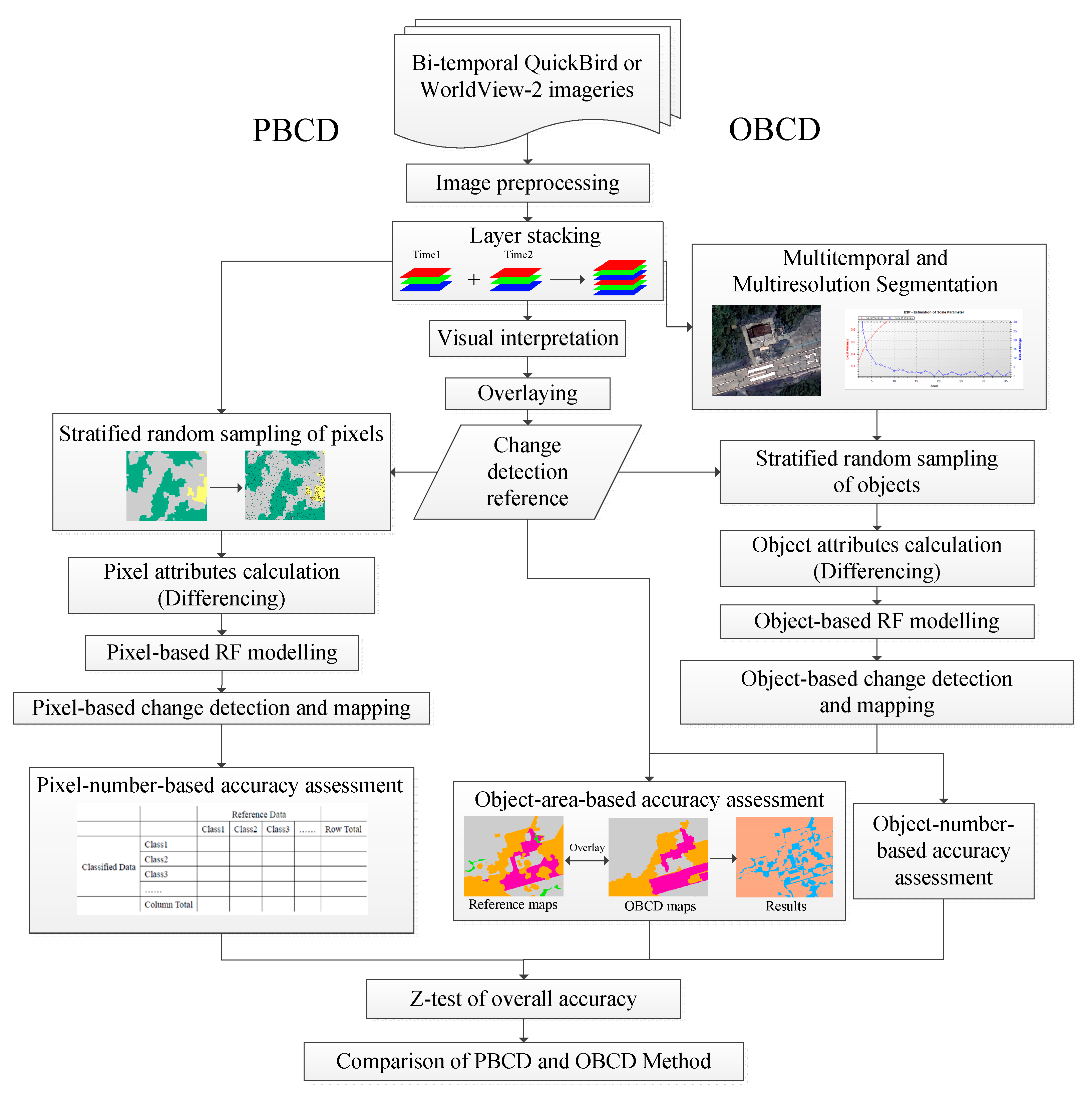
2. Materials and Methods

2.1. Study Area

The South China Sea, which encompasses an area of more than 3 million km2, is the western margin of the Pacific Ocean and the third largest marginal sea in the world. The coastal areas of the South China Sea and its archipelagoes (e.g., the Spratly Islands) provide highly favorable conditions for the growth and development of coral reefs. This region supports 571 known species of reef coral, a richness in biodiversity comparable with that of the Coral Triangle [32]. However, in recent years, the reef islands within this region have undergone complex changes due to both the construction of artificial islands and the effects of natural factors. Therefore, monitoring and studying of the changes in the coral reef environment are very important for marine conservation and management. In this study, we chose Taiping Island, Zhongye Island, and two segments of Barque Canada Reef as study sites (Figure 1), and we monitored dynamics of the reef islands and of the benthic coral habitats.
Zhongye Island (11°03′6″ N, 114°17′12″ E) is of triangular shape, covering an area of roughly 0.372 km2. Zhongye Island has a long history of habitation by fishermen. The island is covered by tropical coastal forests, grasslands, beaches formed by the accretion of carbonate sands and coral shingles, buildings, and roads.
Taiping Island (10°22′37″ N, 114°21′57″ E), located in the northern central region of the Spratly Islands, is a long and narrow island with East-West alignment. The length of the island is approximately 1.4 km and its width is about 0.4 km. Its terrain is low and flat with elevations ranging from 4.0 to 6.0 masl. The land cover types on Taiping Island are similar with Zhongye Island.
Barque Canada Reef (8°10′50″ N, 113°17′41″ E) is an ovular reef that is 33-km long and 5-km wide at its maximum. Its overall area is approximately 66.4 km2 (of which reef flat accounts for 49.5 km2), making it one of the largest of the Spratly Islands. The broad and shallow reef lagoon in the middle of Barque Canada Reef (depth: 1.5–3.0 m) is one of the most important fisheries in the Spratly Islands. Two parts of Barque Canada Reef were selected as study sites for this work. Detailed information (i.e., area of different surface types) of all study sites has been illustrated in Table A1 in Appendix A.

2.2. Data Set and Image Preprocessing

The focus of this study is bi-temporal change detection, so images with pronounced changes between two different times were needed. However, due to the special marine environment and the monsoonal climate [33], the satellite images of the study sites suffered a lot from cloud and aerosol. We have tried to select cloud-free and high-quality images with the data acquisition month close to each other (an interval less than 2 months) in case of pseudo changes or detection errors. Finally, six satellite images over the four study sites were selected as the best available cloud-free scenes, including QuickBird images of Taiping Island acquired in April 2004 and February 2010, QuickBird images of Zhongye Island acquired in April 2005 and June 2010, and WorldView-2 images of Barque Canada Reef acquired in May 2013 and July 2015 (Table 1).
Radiometric correction was firstly conducted for all the images, which is a critical pre-process for change detection. In this study, the digital number values of the satellite images were firstly converted to physically meaningful top-of-atmosphere radiances via radiometric calibration toolbox, following which they were transformed into surface reflectance, using a MODTRAN-based atmospheric algorithm, Fast Line-of-Sight Atmospheric Analysis of Spectral Hyper-cubes (FLAAH) module developed by Spectral Science, Inc., Burlington, NJ, USA. [34]. A further description of atmospheric correction process is provided by the user’s guide [35]. The Gram–Schmidt algorithm was used to fuse the low-resolution multispectral bands with the high-resolution panchromatic band, which resulted in synthetic data with high spatial detail and spectral diversity [36]. For each study site, the image from the earlier time point was registered to the one from the later time point using the ENVI Image Registration Workflow tool, which achieved a registration error of <2 pixels. In this process, tie points were generated automatically according to the geographical coordinates of the images, and a first-order polynomial transformation and nearest neighbor resampling were applied to the earlier image. The accuracy of monitoring and mapping of shallow-water coral reefs is usually compromised by variable water depths. To overcome the influence of bottom reflectance, a kind of depth-invariant index was proposed for water column correction [37]. However, as the study sites of Barque Canada Reef are reasonably shallow (depth: 1.5–3.0 m), water column correction was deemed unnecessary in such case [38]. Furthermore, as the focus of this study was on the detection of relative changes between two periods, the effects of water depth were deemed negligible.
All the six remote sensing images were interpreted visually by digitalizing and classifying the whole scenes. Then, we overlaid two digitalized images of each study site and generated a new layer. In the generated layer, polygons with attributes from two different times were defined as “no change” or as a certain change category according to its types in two different times. The definition rules of two reef islands are shown in Table 2 and those of Barque Canada Reef are shown in Table 3. In the reef islands, change categories include vegetation deterioration, vegetation growth or plantation, coastal accretion, sea level rise or coastal erosion, and others. The “others” category refers to changes related to buildings and infrastructure construction, e.g., house building, runway or road construction, coastal harbor construction, etc. Areas without surface type change were categorized as “no change”. In the Barque Canada Reef study sites, changes refer to alterations in species assemblages and in their associated substrata extent [39]. These changes were categorized as aquatic vegetation growth, algae growth, reef sediments extension, and algae degradation. Areas without habitat type change were categorized as “no change”. After defining the change categories, the overlaid layer of each study site was used as reference data for sampling in both OBCD and PBCD methods and for object-area-based accuracy assessment. The area and proportion of each change category in all study sites are displayed in Table A2 and Table A3 in Appendix A.
A detailed schematic of all experimental procedures including image preprocessing has been presented in Figure 2. Compared to PBCD, the OBCD method includes an additional key step of image segmentation, which is described in detail in Section 2.3.1. Finally, the change detection performances of the two methods are compared in terms of the overall accuracy (OA), Producer’s accuracy (PA), User’s accuracy (UA), Kappa coefficient (KA), and Z-test.

2.3. Object-Based Coral Reef Change Detection

2.3.1. Multi-Temporal Segmentation

Image segmentation is at the core of the OBIA method because the object obtained from image segmentation is the basic unit used for image classification or change detection. Thus, the quality of image segmentation is correlated strongly with the accuracy of image classification and change detection [40]. Multiresolution segmentation is a regional merging algorithm that forms an image object starting from a single pixel. At each step, a pair of small image objects will be selected for merging into a larger object or not based on a homogeneity criterion that is defined by the scale parameter (SP), color/shape weight, and smoothness/compactness weight. As the SP determines the average size of the image objects according to the heterogeneity within the object, the SP selection is crucially important [41]. Based on the rate of change of local variance (ROC-LV) concept [42], an automatic tool called “Estimate of Scale Parameter” (ESP) has been proposed as particularly suitable for replacing the subjective trial-and-error method in SP selection [43,44]. The local variance (LV) value reflects the heterogeneity within an object. Its value increases incrementally with the increasing segmentation scale up to a point, at which the ROV-LV reached a peak. The SP at this point is considered the optimal segmentation scale and the object obtained from the segmentation approximates the actual ground object.
In this work, segmentation was conducted on all images of different dates simultaneously after stacking all sets of the spectral bands. This multi-temporal image segmentation approach unifies the object boundaries of all sequential images, minimizing sliver errors and delineating objects that are composed of spatially adjacent pixels with similar spectral properties over time [19,45].
The ESP tool has been programmed in CNL within the eCognition® Developer 9.0 environment. The ESP2 plugin in eCognition® Developer 9.0 was used to perform multiresolution segmentation in a hierarchical manner with default scale increments of 1, 10, and 100 and a step size of 1. The values of shape weight and compactness weight were set as 0.1 and 0.5, respectively. ROC-LV curves were produced using standalone software. As an example, the optimal segmentation scale of Zhongye Island was established as 13, as was shown in Figure 3.

2.3.2. Object Feature Selection and Calculation

Each image object has its own spectral, spatial, and textural features that are fundamental elements in human interpretation of color photographs [46]. The state of each object at different time points can be described using a given set of features [47]. In Equation (1), St1 represents the state (or land cover type) of an object at time t1, and F1, F2, … Fn is the feature set of t1. St2 represents the state (or land cover type) of an object at time t2, and F1’, F2’, … Fn’ is the feature set of t2. ∆S is the difference between the features of the object at t1 and t2. Using feature differences to train the change detection model halves the dimensionality of the dataset and reduces the necessary computations [48].
S t 1 = ( F 1 F 2 F 3 F n ) S t 2 = ( F 1 F 2 F 3 F n ) Δ S = ( F 1 F 1 F 2 F 2 F 3 F 3 F n F n )
After multi-temporal segmentation, the objects in the segmented images have consistent geometries and sizes between different times. Hence, only the spectral and textural features of each object were considered for change detection. For better recognition of changes in vegetation and water bodies, the Normalized Difference Vegetation Index (NDVI) [49] and Normalized Difference Water Index (NDWI) [50] were calculated as additional feature bands for both Taiping Island and Zhongye Island using band algebra. The object features of both Zhongye Island and Taiping Island included the mean values and standard deviations of the blue, green, red, near infrared, NDVI, and NDWI bands. Haralick texture features including GLCM homogeneity, GLCM contrast, GLCM dissimilarity, GLCM entropy, GLCM Ang. 2nd moment, GLCM correlation, GLDV Ang. 2nd moment, GLDV entropy, and GLDV contrast [51]. As the study sites on Barque Canada Reef were located in shallow water, we calculated only the mean values and standard deviations of the three visible bands, i.e., the blue, green, and red bands that can penetrate shallow water [30], together with the nine Haralick texture features. All these features were calculated in eCognition® Developer 9.0.

2.3.3. Sampling Changed Objects

In order to implement stratified random sampling, we first labelled all segmented objects using a maximum overlay rule with reference layer, where all changes or no changes are depicted for individual study site (see Section 2.2). Each segmented object was defined as the class displayed in the reference layer that covered the majority area of this object. Subsequently, all segmented objects were divided into groups according to their change types. Then, each stratum was randomly sampled with the same training set ratio of 30%. For Zhongye Island, 902 segmented objects were selected for training samples. For Taiping Island, 1101 segmented objects were selected for training samples. The training samples of the two study sites in Barque Canada Reef were 2843 and 3436 image objects, respectively. The remaining 70% objects were used as validation samples. Sample numbers of each change category have been displayed in Table A4 and Table A5. As the sampled units were polygonal objects, there could have been variety in the training sample objects’ size. Therefore, we made appropriate adjustments to the sampling results through visual observation, such that the training samples were representative both in change type and in size.

2.3.4. Recognizing Changed Objects Using the RF Algorithm

The RF algorithm [52] is a powerful ensemble learning technique that has been used widely in remote sensing image classification [53,54]. Its superiority to other machine learning methods (e.g., decision tree classifier, neural network classifier, maximum likelihood classifier, etc.) has been demonstrated in a number of earlier studies [53,55,56]. In a lot of studies, RF classifier performed equally well to SVMs in terms of classification accuracy and training time [57,58,59], but RF was acknowledged more user-friendly for the number of user-defined parameters required by RF classifiers is less than the number required for SVMs and easier to define [60]. The RF algorithm has not only been applied successfully in pixel-based image analyses, but has also shown great promise in the OBIA method for its high accuracy [61] and robustness to training sample reduction and feature selection [62,63]. Therefore, the RF algorithm was adopted in the current work.
The RF algorithm was implemented in the RandomForest package in the R environment [64]. The input predictive variables were difference values of object features between two time points, including the difference of mean values and standard deviations of the blue, green, red, near infrared, NDVI, and NDWI bands, the Haralick texture features, as was mentioned above. The predicting result was the change category. Before training a RF model, two primary parameters of RF algorithm need to be defined: the number of trees ntree and the number of split variable parameters mtry. A review of RF application in remote sensing concluded that in most studies, the errors stabilize before ntree value reaches 500, so the default value of 500 for ntree is an acceptable value [65]. The other parameter mtry is the number of prediction variables used in each node to make the tree grow. According to Rodriguez-Galiano, et al. [66], a RF is not sensitive to the value of mtry as the generalization error converges from the value of approximately 100 trees. Moreover, it was found that using a univariate RF algorithm could produce good accuracy and save computation time [52]. Therefore, this paper set ntree as 500 and set mtry as 1. In this study, four separate RF models were established to detect changes in four study sites.

2.4. Pixel-Based Coral Reef Change Detection

The same fundamental procedures (e.g., stratified random sampling and RF change detection) were used in the PBCD method, with the exception of image segmentation. Here the basic unit of the PBCD method is a pixel rather than an object. Therefore, we directly sampled the pixels labelled by the reference layer for each category, and each stratum was randomly sampled with the same training set ratio as object-based method. Subsequently, the training samples and validation samples of each change category were collected based on the same proportion as object-based method (still 30% training samples and 70% validation samples for each category). In this process, a total number of 42,276 pixels and 69,846 pixels were selected in Taiping Island and Zhongye Island, respectively. A total number of 460,960 pixels and 459,120 pixels were selected in Barque Canada Reef Site 1 and Site 2. The sample numbers of each change category in all the study sites have been shown in Table A6 and Table A7. The pixel-based RF change detection models were also trained and constructed using the RandomForest package in the R environment with the parameter ntree set as 500 and the parameter mtry set as 1. For Zhongye Island and Taiping Island, the pixel value difference of the blue, green, red, near infrared, NDVI, and NDWI bands was input as predictive variables to predict change types. For the study sites on Barque Canada Reef, the pixel value difference of the blue, green, and red bands was chosen as predictive variables. Ultimately, we obtained change detection results for the entire image of each study site with the aid of RF change detection models.

2.5. Accuracy Assessment and Statistical Comparisons

2.5.1. Confusion Matrix Based on Pixel Number, Object Number, and Object Area

For each of the four study sites, three confusion matrices were created based on pixel number, object number, and object area in order to calculate the OA, PA, UA, and Kappa coefficient. In the PBCD method, the values in the rows and columns of the confusion matrices refer to pixel numbers. To analyze quantitatively the classification quality of object-based methods, Laliberte and Rango [67] considered each object as an element, and generated confusion matrices based on the object numbers. However, this method was deemed spatially implicit [68]. Thematic accuracy and completeness as well as geometric quality and integrity were suggested prerequisites for comprehensive analysis of object-based classification quality [69]. Whiteside, et al. [70] proposed an area-based validation method, in which reference layer R is superimposed on the change detection product C. Their overlap, |Ci∩Ri| represents the correctly identified part of change type i, whereas |Ci∩¬Ri| represents the commission part of change type i and |¬Ci∩Ri| is the omission part of change type i. In this case, the values in the rows and columns of the confusion matrices refer to the areas of these parts. In this work, a pixel-number-based confusion matrix was used to assess the PBCD accuracy, whereas confusion matrices based on object number and object area were used to assess the OBCD accuracy.

2.5.2. Statistical Hypothesis Test for PBCD and OBCD Accuracy Assessment

To determine whether the RF change detection models in the PBCD and OBCD methods yielded significantly better results than random ones, a Z-test was performed on the Kappa coefficient of each confusion matrix. In addition, the Kappa coefficients of the OBCD and PBCD confusion matrices were analyzed using a Z-test. This was performed to check for significant differences between the accuracies of the two methods [71] in order to determine whether the OBCD method was significantly superior.
Here, K1 and K2 denote the KA coefficients of the two confusion matrices, while var (K1) and var (K2) denote the variances of K1 and K2, respectively. The Z-test statistic for testing the significance of a single confusion matrix is calculated as follows:
Z 1 = K 1 var ( K 1 )  
where Z1 is a standard normal deviate. The null and alternative hypotheses are formulated as follows: H0: K1 = 0, H1: K1 ≠ 0; H0 is rejected if Z ≥ Zα/2, where a/2 is the confidence level.
The Z-test statistic for testing whether two independent confusion matrices are significantly different can be expressed as
Z 12 = | K 1 K 2 | var ( K 1 ) + var ( K 2 )  
where Z12 is a standard normal deviate. The null and alternative hypotheses are formulated as follows: H0: (K1K2) = 0, H1: (K1K2) ≠ 0; H0 is rejected if Z ≥ Zα/2.
At the 95% (99%) confidence level, the critical value would be 1.96 (2.58). For a single confusion matrix test, a value of the Z statistic > 1.96 means the result is significant (i.e., better than random) at the 95% confidence level. For a test between two confusion matrices, a value of the Z statistic > 1.96 means the results are significantly different, i.e., one method outperformed the other.

3. Results

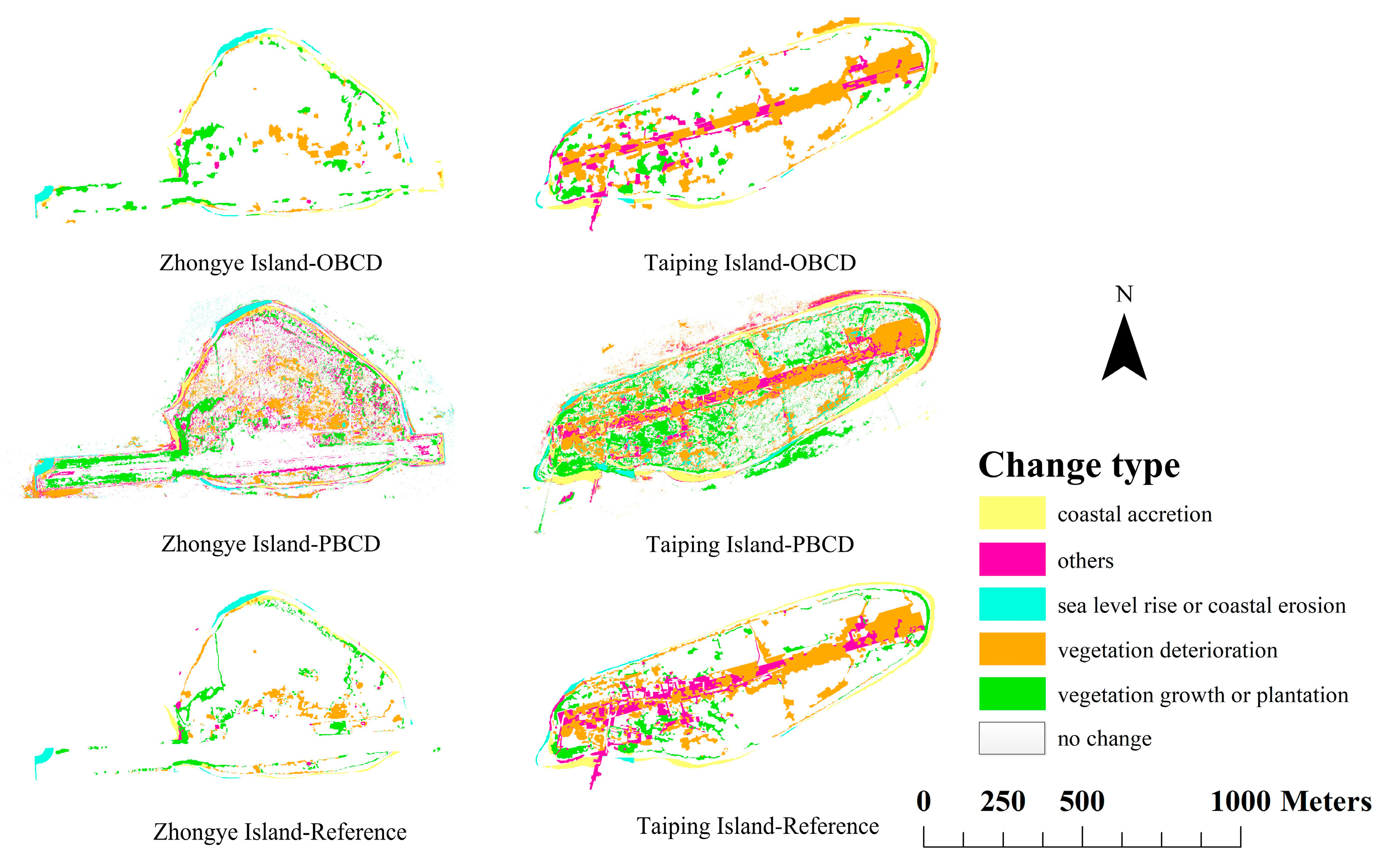
3.1. Visual Examination of PBCD and OBCD Maps

The outputs of the change detection methods for the four study sites are shown in Figure 4 and Figure 5. Visual comparison revealed that both the OBCD and the PBCD methods were able to recognize changed areas and change types. Nonetheless, the OBCD method appeared to outperform the PBCD method. Specifically, the OBCD maps were not affected severely by salt-and-pepper effects and very few unchanged areas were misidentified as changed.

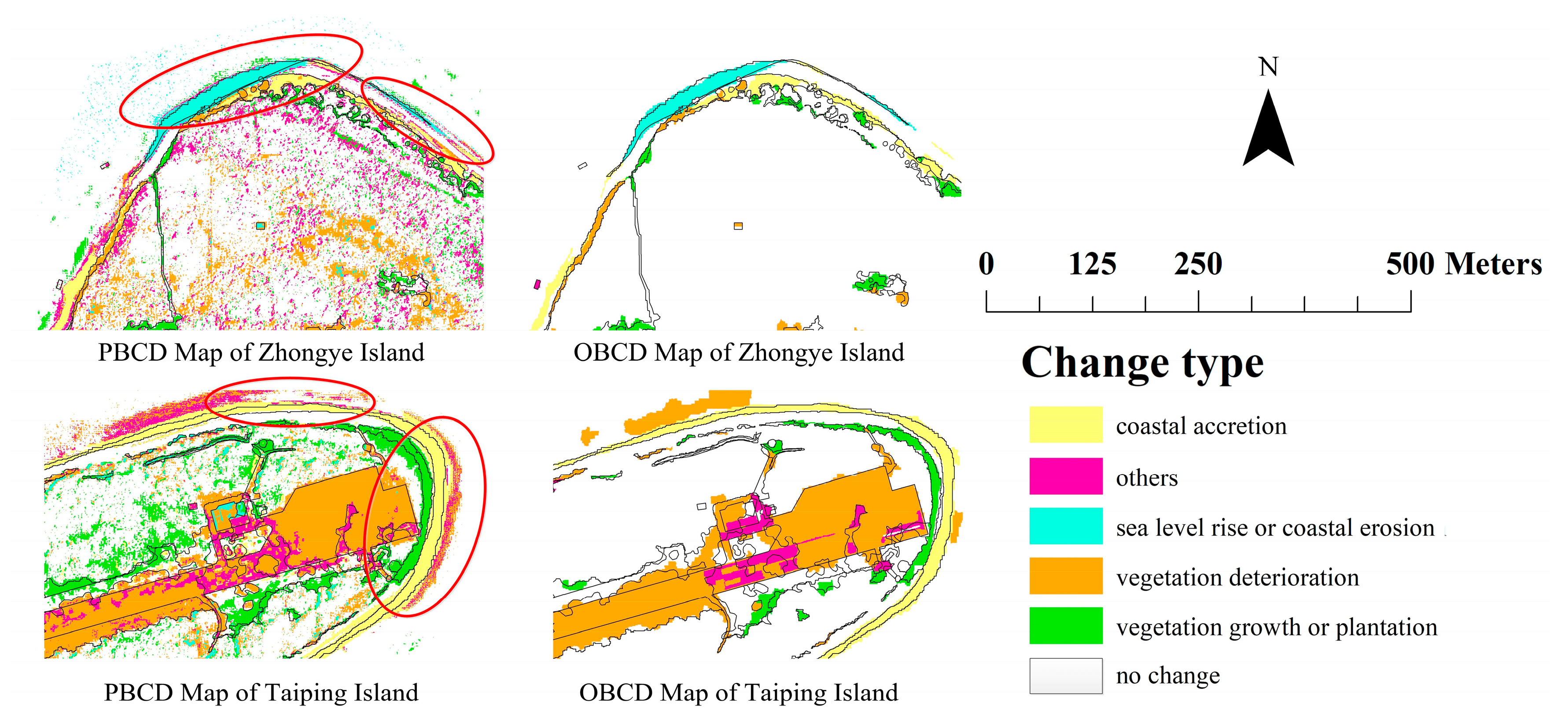
3.1.1. An Observation of PBCD Maps

The changed areas recognized by the PBCD method were irregular clusters of pixels. Furthermore, pixels of various change types were distributed sporadically within the areas of certain other change types. For example, the areas of “vegetation deterioration” detected on both Taiping Island and Zhongye Island also contained scattered pixels of the “others” change type. We also found that PBCD frequently detected unchanged areas as changed. On both Taiping Island and Zhongye Island, the surrounding stable (unchanged) marine areas were identified as “vegetation growth or plantation”, “vegetation deterioration”, and “others”. A proportion of unchanged forest on Zhongye Island was identified as “vegetation deterioration” and “others”, while central areas of Taiping Island, where no change occurred, were detected mostly as “vegetation growth or plantation”. The PBCD method presented the worst visual accuracy for both study sites of Barque Canada Reef. In Barque Canada Reef Site 1, large areas of “no change” type were misidentified as “aquatic vegetation growth” and “algae growth”, while substantial proportions of “no change” areas in Barque Canada Reef Site 2 were misidentified as “aquatic vegetation growth”.

3.1.2. An Observation of OBCD Maps

In stark contrast to the PBCD method, the OBCD method produced much cleaner and neater change detection maps with the polygon as its basic analysis unit. Of the four study sites, the change detection map of Zhongye Island was found most similar with its reference layer, although minor changes such as vegetation growth on narrow paths were not detected well. The change detection map for Taiping Island was also satisfactory, except that some unchanged marine areas to the north of the reef island were misidentified as “vegetation deterioration” shown as conspicuous orange patches. Patches of unchanged area in eastern parts of Barque Canada Reef Site 1were misidentified as “algae growth”, while a scattering of unchanged polygons in the middle of Barque Canada Reef Site 2 were detected as “aquatic vegetation growth”. The results revealed that the primary weakness of the OBCD method was that there were discrepancies between the boundaries of its change detection units (image objects) and the polygonal boundaries in the reference layer, which delimited the actual change extent.

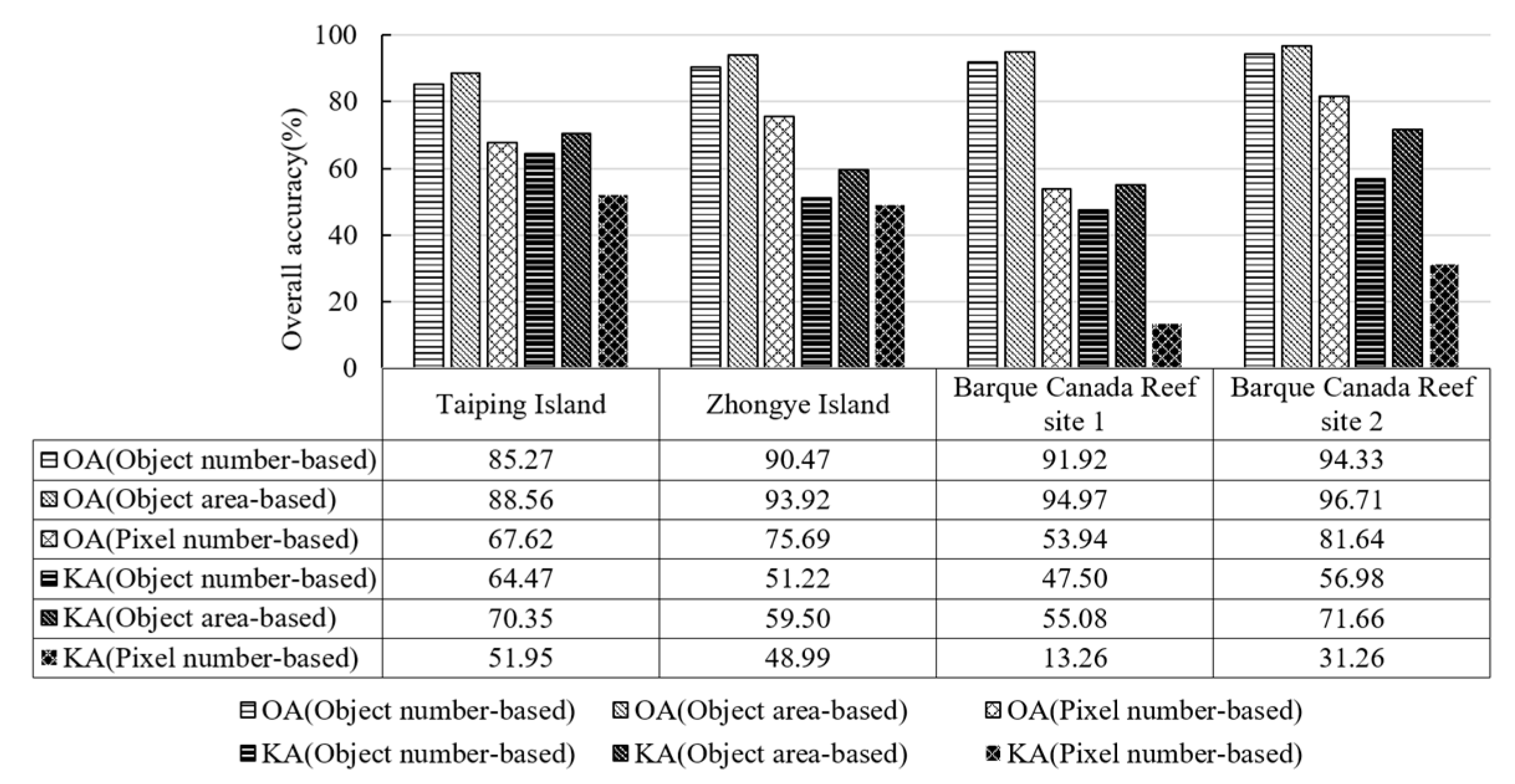
3.2. Quantitative Evaluations of PBCD and OBCD Performances

3.2.1. PBCD and OBCD Accuracy Assessment

Three confusion matrices based on pixel number, object number, and object area were used to assess the accuracy of each change detection result. Figure 6 illustrates the OAs and the Kappa coefficients of the OBCD and PBCD methods for each study site. Table 4, Table 5, Table 6 and Table 7 display all the confusion matrices. It was found that the OAs of OBCD, either object-number or object-area based, were greatly higher than those of PBCD for all the study sites. Meanwhile, the object-area-based OA was a little bit higher than the object-number-based OA. The average OA of OBCD over the four study sites was >90%, i.e., approximately 20% higher than the average OA of PBCD (69.72%). The OBCD method was effective for the reef islands and coral reef habitats change detection, achieving OAs > 90%, except for Taiping Island, whose OA was only slightly >85%. The accuracy assessment results revealed that the PBCD method did worse in benthic coral reef environment than in reef islands. This was particularly reflected in the PBCD Kappa coefficients of the two reef islands and the Barque Canada Reef study sites.
The PBCD results of all the study sites indicated that the UAs for all change types (except “no change”) were <60%, i.e., the commission errors of PBCD were >40%. In Barque Canada Reef study sites, except for “no change” category, the other change categories got greatly worse pre-class UAs. For example, the UA of “reef sediments extension” type was only 24.9% in Barque Canada Reef Site 1 while the “no change” type got a high UA (99.3%). Although per-class UAs of certain categories in object-number-based accuracy assessment were higher than those of pixel-number-based accuracy assessment, some of the rest categories got even lower UAs. In the object-area-based accuracy assessment, the UAs of all the other change types were lower than “no change” type. Nonetheless, per-class UAs of all change categories were higher than those obtained from the object-number-based and pixel-number-based confusion matrices. What’s more, the area-based assessment produced a much more balanced per-class UAs of all change categories. For example, in Taiping Island, area-based UAs of all change categories approximated 70%. For the Barque Canada Reef study sites, UAs of all change categories were greatly improved and much closer to each other.
In the change detection results of the two reef island sites, the “others” category consistently displayed the lowest accuracy. Many changes in the “others” category were identified erroneously as “no change”, “vegetation deterioration”, or “vegetation growth or plantation”. For Zhongye Island, the UA of the “others” type was relatively low, i.e., the PBCD method had a UA of 2.9%. In the validation samples of object-number-based accuracy assessment, not a single “other” category object was correctly recognized. The confusion matrices of the OBCD method revealed that “aquatic vegetation growth” and “algae growth” were difficult to distinguish from one another, because the UAs of the OBCD method for “aquatic vegetation growth” and “algae degradation” were relatively low, and the object-number-based accuracy was even lower than the object-area-based accuracy.

3.2.2. Z-Test Results of the Accuracy Assessment

As shown in Table 8, the Z-test values of all the individual confusion matrices (especially the area-based OBCD confusion matrices) far exceeded 2.58 (p ≤ 0.01) and 1.96 (p ≤ 0.05), indicating that the RF algorithm combined PBCD and OBCD methods are both feasible and effective, and that the change detection results were significantly better than random results. Comparisons between the object-number-based OBCD assessment result and the PBCD assessment result revealed no significant differences for Zhongye Island (|Z| = 0.60 < 1.69), but the Z-test values for the other study sites were much larger than 2.58 (p ≤ 0.01) and 1.96 (p ≤ 0.05). Comparing the object-area-based assessment results and the pixel-number-based results, the Z-test values for all study sites were far greater than 2.58 (p ≤ 0.01) and 1.96 (p ≤ 0.05), i.e., the object-area-based accuracy was significantly higher than that of PBCD.

4. Discussion

4.1. Pros and Cons of the Proposed OBCD Method

The proposed OBCD method segmented images from two different times together and then trained RF models using difference of object features to predict change category. The advantages of this method are evident. First, since change categories were defined in advance, changed areas and the corresponding change categories can be directly recognized using a one-step supervised classification. Secondly, the RF algorithm has high computational speed and helps optimizing the classification model by using only the input object features as predictive variables [65] compared to traditional rule-based method or pixel-based method. Changes can be detected in a more automatic way than with the membership rules method, which sets individual threshold values of classification rules iteratively based on expert knowledge and by visually comparing the image objects with field data [17,18]. Moreover, the algorithm running time of OBCD is obviously shorter than that of PBCD. In the PBCD method, the training sample size generally amounts to tens of thousands of pixels, while the training sample size for the OBCD method were only tens or hundreds of objects. Therefore, the average running time of the RF model for PBCD is about hundreds of seconds, while RF model building and change prediction could be accomplished within seconds for the OBCD method (not shown here). Thirdly, the method also achieved a high change detection accuracy (over 85%) for all the coral reef study sites, which confirms a good transferability of this workflow.
The proposed method also has some weakness. Small or indistinct changes cannot be easily detected due to the multi-temporal segmentation, where these changes may be merged into large objects in the segmentation process [72]. Despite the high overall accuracy, there was a great difference between per-class accuracy. Expect for the “no change” category, accuracies of other change categories were not as high as the accuracy recommended for creating an inventory of resources for management [73]. The imbalance of samples may have influence on the per-class accuracy. Classification trees suffer from unbalanced sample sizes because the largest number of samples tend to determine the class label [74]. On the other hand, challenges in respect of the quantity and quality of the training samples also affect the performance of the supervised classification [75]. In the reef island sites, the “others” category always had the lowest accuracy, while the “no change” type, which accounted for the largest area of each study site, gained the highest accuracy. Changes of the “others” type relate to human development and reconstruction activities. Buildings and infrastructures on reef islands take various shapes and forms with distinctive spectral and textural properties, which greatly increased the uncertainty of the training samples in the supervised change detection. In addition, the number of training samples of “others” type obtained via proportional stratified sampling was quite small because of the limited extent of the changes. For example, in Taiping Island, the training samples of “others” type were 52 objects for object-based change detection and 357 pixels for pixel-based method as the area of “others” change type occupied only 4.98% of the entire study site. By contrast, there were 684 training objects and 13,218 training pixels of “no change” type.

4.2. The Superiority of the OBCD Method to the PBCD Method

A comparison of PBCD and OBCD showed that object-based paradigm is superior to the pixel-based paradigm for detecting changes from very-high-resolution satellite images of coral reefs. The OA of the OBCD method was about 20% greater than the PBCD method, similar to the findings derived by Benfield et al. [30] in their coral reef classification study. Cleve et al. [76] also found that the object-based classification approach provided a 17.97% higher OA than the pixel-based approach in wildland–urban interface classification. However, studies based on medium-resolution satellites such as Landsat and SPOT, concluded that the results achieved by pixel-based methods are acceptable, with no significant difference from the object-based methods [28,31]. As the spatial resolution of remote sensing imagery continues to improve, within-class spectral heterogeneities increase as well, which greatly affect the accuracy of conventional pixel-based methods. In this study, this problem was manifested in the form of severe salt-and-pepper effects and numerous misidentified pixels in the PBCD maps. The PBCD method recognizes changes based solely on pixel values, which are susceptible to interference from other factors. Factors including light conditions, tree shade, vegetation phenology, etc. might induce changes in the spectral features of pixels, thus leading to the detection of spurious changes. By comparison, the OBCD method analyzes the overall properties of all pixels within an object. Thus, changes of individual pixels have minimal impact on the general features of an object, making the OBCD method more robust and reliable.

4.3. Application of PBCD and OBCD Methods in Multiple Coral Reef Study Areas

The complicated formation process and the special location render coral reef islands spatiotemporally dynamic [77] and vulnerable to climate change and sea level rise [78]. Much attention has been paid to the dynamics of atoll islands. Historical aerial photographs or satellite images with different spatial resolution over a period of time were usually rectified to each other and digitalized to investigate the stability of vegetated cays or islands [79]. However, in most cases, atoll islands have a paucity of distinct and stable features for ground control points, rendering georeferencing of images problematic [80]. Besides, differing resolution or quality of time series images may affect the accuracy of the image registration and shoreline interpretation, and thus impact change detection accuracy. In our study, the proposed OBCD method was less prone to image misregistration than the PBCD method, as was observed from both the generated map and the accuracy. Using the PBCD method, pixels between neighboring segments tended to be misclassified, generating an obvious dividing line with a width of several pixels (Figure 7). Using the OBCD method, registration error did not cause fragmented objects. According to Chen, Zhao, and Powers [21], when the registration error is relatively small (e.g., lower than 3 pixels), the size of image objects slightly increased, because small objects were merged into the neighboring image-objects. Since misregistration had a low impact on object size and shape for most areas, the change detection accuracy would remain at a high level.
For the Barque Canada Reef study sites, it was found that PBCD methods were less suitable for coral reef community at a coarse scale, due to the serious salt and pepper effects in the change detection maps. In addition, it was found challenging to distinguish “aquatic vegetation growth” and “algae growth”. Seagrass and algae may have similar textural features and similar spectral characteristics using only the red, green, and blue bands. It has been suggested that hyperspectral data could provide for a more detailed and accurate classification or change detection of reef biotic systems, because it can provide rich information on the reflectance properties of algal and seagrass communities [81].

4.4. Object-Number-Based and Object-Area-Based Accuracy Assessment

In this work, we used two different accuracy assessment methods to evaluate the OBCD results. The object-area-based assessment of OBCD got a slightly higher OA than the object-number-based assessment and a greatly higher OA than the pixel-number-based assessment. Besides, the per-class accuracy of each change category was higher and more balanced in the object-area-based assessment. Although the OA of the object-number-based assessment was also greatly higher than the per-pixel results, the per-class accuracy did not show superiority. Two main reasons may account for all the findings above. First, in the object-based paradigm, image segmentation inevitably results in mixed objects; thus, once an object is misidentified, the object-number-based change detection accuracy will be lowered significantly, especially for change types with a small number of total samples. Second, the average size of correctly identified objects might be bigger than objects of incorrectly identified objects in almost all classes [82], so the final overall accuracy of object-area-based assessment was higher than the object-number-based accuracy. If the classified objects are imported to GIS for a further spatial analysis, both the thematic and geometric accuracy assessment are necessary and important. The object-area-based assessment is essentially a comprehensive evaluation of image segmentation and change detection, which is not only influenced by the classification algorithm, but also strongly relates to the segmentation means. Therefore, more combinations of classification algorithms and segmentation means need to be further explored.

5. Conclusions

As image registration is critical but challenging in coral reef change detection because of the deficiency of distinct and stable texture features as well as ground control points, in this work, we proposed an RF-combined object-based framework for change detection in coral reef environment and we applied this framework to multiple coral reef study sites in the South China Sea. The combination of multi-temporal object-based analysis and the RF algorithm not only recognized changed areas, but also offered information about the corresponding change types. The OBCD method achieved a high accuracy in coral reef environment with a good transferability over various study sites. Through a comparison analysis, it was found that the OBCD method significantly outperformed the PBCD method. The OBCD method did not suffer from salt-and-pepper effects and it was less sensitive to image misregistration than the PBCD method. Therefore, the OBCD method is more suitable for coral reef environment monitoring. The object-area-based assessment of OBCD produced a higher OA than both the object-number-based assessment and the pixel-number-based assessment. Besides, per-class accuracy of the object-area-based assessment was higher and more balanced. For further GIS analysis or statistical analysis, the object-area-based accuracy assessment should be considered.
There were some shortcomings of this work. Given the high cost of field data collection, we had to visually interpret digitized high-resolution remote sensing images to obtain the reference layers. Thus, the change detection scale of this study was relatively coarse and the classification system of the change types was simple, especially for the Barque Canada Reef study sites. In future work, this framework could be tested on other coral reef images with rich validation information to realize change detection on finer scales with finer classification systems.

Author Contributions

All authors contributed to this paper. L.M. conceived and designed the experiments, and also contribute to the manuscript writing; Z.Z. performed the experiments, results interpretation, and manuscript writing; T.F., M.Y. and G.Z. assisted with the experimental result analysis; M.L. contributed images/materials/analysis tools.

Funding

This work was supported by the National Key R&D Program of China (No. 2017YFB0504200), the National Natural Science Foundation of China (No. 41701374), the Natural Science Foundation of Jiangsu Province of China (No. BK20170640), and the China Postdoctoral Science Foundation (No. 2017T10034, 2016M600392).

Acknowledgments

We are grateful to anonymous reviewers and members of the editorial team for advice.

Conflicts of Interest

The authors declare no conflict of interest.

Appendix A

Table A1. The area and proportion of reef island surface and coral reef habitats.
Zhongye Island
TypesArea in 2005 (m2)Proportion in 2005 (%)Area in 2010 (m2)Proportion in 2010 (%)
Buildings and infrastructures154,819.8624.85145,485.3523.35
Ocean237,918.2938.18237,576.7438.13
Bare land35,529.865.7035,064.845.63
Beach20,092.133.2226,716.404.29
Vegetation174,709.0928.04178,225.9128.60
Sum623,069.23100.00623,069.23100.00
Taiping Island
TypesArea in 2004 (m2)Proportion in 2004 (%)Area in 2010 (m2)Proportion in 2010 (%)
Buildings and infrastructures67,932.389.17127,455.0817.20
Ocean323,486.8643.65313,509.6442.31
Bare land34,235.364.6242,485.035.73
Beach37,762.435.1050,523.226.82
Vegetation277,608.1037.46207,052.1727.94
Sum741,025.13100.00741,025.13100.00
Barque Canada Reef Site 1
TypesArea in 2013 (m2)Proportion in 2013 (%)Area in 2015 (m2)Proportion in 2015 (%)
Algae-dominated117,799.305.23316,069.0814.04
Lagoon235,411.5010.467519.960.33
Ocean462,830.4420.56220,900.089.81
Coral-dominated270,640.0812.02241,113.9910.71
Sand400,262.3417.78485,582.7121.57
Rubble-dominated763,992.3533.94225,862.7810.03
Aquatic vegetation753,887.3933.49
Sum2,250,936.00100.002,250,936.00100.00
Barque Canada Reef Site 2
TypesArea in 2013 (m2)Proportion in 2013 (%)Area in 2015 (m2)Proportion in 2015 (%)
Algae-dominated11679.000.3633,324.131.03
Ocean715,696.9122.03720,942.4522.19
Coral-dominated551,229.0016.97500,371.9715.40
Rubble-dominated868,028.6726.72892,846.0027.48
Sand1,102,457.9933.931,000,743.9330.80
Aquatic vegetation100,863.093.10
Sum3,249,091.57100.003,249,091.57100.00
Table A2. The area and proportion of all change categories in Zhongye Island and Taiping Island.
Change CategoriesZhongye IslandTaiping Island
Area (m2)Proportion (%)Area (m2)Proportion (%)
Coastal accretion13,485.462.1616,761.462.26
No change517,984.6983.13577,412.2077.92
Others1490.030.2436,902.004.98
Sea level rise or coastal erosion5327.200.852813.150.38
Vegetation deterioration39,262.326.3081,149.2810.95
Vegetation growth or plantation45,519.537.3125,987.053.51
Sum623,069.23100.00741,025.13100.00
Table A3. The area and proportion of all change categories in Barque Canada Reef.
Change CategoriesBarque Canada Reef Site 1Barque Canada Reef Site 2
Area (m2)Proportion (%)Area (m2)Proportion (%)
Algae growth73,015.263.24%21,655.810.67
Aquatic vegetation growth7475.630.33%100,852.413.10
Reef sediments extension20,314.330.90%30,428.520.94
Algae degradation8006.500.36%
No change2,141,469.5495.16%3,096,154.8795.29
Sum2,250,281.25100.00%3,249,091.60100.00
Table A4. The object sample numbers of all change categories in Zhongye Island and Taiping Island.
Change CategoriesZhongye IslandTaiping Island
TrainingValidationTrainingValidation
Coastal accretion17392866
No change102323866841596
Others2552121
Sea level rise or coastal erosion1126512
Vegetation deterioration2148100234
Vegetation growth or plantation28653376
Sum110125699022105
Table A5. The object sample numbers of all change categories in Barque Canada Reef.
Change CategoriesBarque Canada Reef Site 1Barque Canada Reef Site 2
TrainingValidationTrainingValidation
Algae growth1032404093
Aquatic vegetation growth716128299
Reef sediments extension307169161
Algae degradation818
No change2695629031997466
Sum2843663534368019
Table A6. The pixel sample numbers of all change categories in Zhongye Island and Taiping Island.
Change CategoriesZhongye IslandTaiping Island
TrainingValidationTrainingValidation
Coastal accretion453105812412895
No change982822,93313,21830,843
Others72169357834
Sea level rise or coastal erosion19144613763211
Vegetation deterioration765178431117259
Vegetation growth or plantation1373320316503850
Sum12,68329,59320,95448,892
Table A7. The pixel sample numbers of all change categories in Barque Canada Reef.
Change CategoriesBarque Canada Reef Site 1Barque Canada Reef Site 2
TrainingValidationTrainingValidation
Algae growth651815,20917254025
Aquatic vegetation growth4711098440410,277
Reef sediments extension1814423324075616
Algae degradation6451506
No change128,840300,626129,200301,466
Sum138,288322,672137,736321,384

References

  1. Moberg, F.; Folke, C. Ecological goods and services of coral reef ecosystems. Ecol. Econ. 1999, 29, 215–233. [Google Scholar] [CrossRef]
  2. Reaka-Kudla, M.L. The global biodiversity of coral reefs: A comparison with rain forests. In Biodiversity II: Understanding & Protecting Our Biological Resource, 2nd ed.; Reaka-Kudla, M.L., Wilson, D.E., Wilson, E.O., Eds.; Joseph Henry/National Academy Press: Washington, DC, USA, 1997; pp. 83–108. [Google Scholar]
  3. Folke, C. Confronting the coral reef crisis. Nature 2004, 429, 827. [Google Scholar]
  4. Burke, L.M.; Reytar, K.; Spalding, M.; Perry, A.L. Reefs at risk revisited. Ethics Medics 2011, 22, 2008–2010. [Google Scholar]
  5. McCarthy, M.J.; Colna, K.E.; El-Mezayen, M.M.; Laureano-Rosario, A.E.; Mendez-Lazaro, P.; Otis, D.B.; Toro-Farmer, G.; Vega-Rodriguez, M.; Muller-Karger, F.E. Satellite remote sensing for coastal management: A review of successful applications. Environ. Manag. 2017, 60, 323–339. [Google Scholar] [CrossRef] [PubMed]
  6. Yamano, H.; Tamura, M. Detection limits of coral reef bleaching by satellite remote sensing: Simulation and data analysis. Remote Sens. Environ. 2004, 90, 86–103. [Google Scholar] [CrossRef]
  7. Palandro, D.A.; Andréfouët, S.; Hu, C.; Hallock, P.; Müller-Karger, F.E.; Dustan, P.; Callahan, M.K.; Kranenburg, C.; Beaver, C.R. Quantification of two decades of shallow-water coral reef habitat decline in the florida keys national marine sanctuary using landsat data (1984–2002). Remote Sens. Environ. 2008, 112, 3388–3399. [Google Scholar] [CrossRef]
  8. El-Askary, H.; Abd El-Mawla, S.H.; Li, J.; El-Hattab, M.M.; El-Raey, M. Change detection of coral reef habitat using landsat-5 TM, Landsat 7 ETM+ and Landsat 8 OLI data in the red sea (Hurghada, Egypt). Int. J. Remote Sens. 2014, 35, 2327–2346. [Google Scholar]
  9. Mumby, P.J.; Green, E.P.; Edwards, A.J.; Clark, C.D. The cost-effectiveness of remote sensing for tropical coastal resources assessment and management. J. Environ. Manag. 1999, 55, 157–166. [Google Scholar] [CrossRef]
  10. Scopélitis, J.; Andréfouët, S.; Phinn, S.; Done, T.; Chabanet, P. Coral colonisation of a shallow reef flat in response to rising sea level: Quantification from 35-years of remote sensing data at Heron Island, Australia. Coral Reefs 2011, 30, 951–965. [Google Scholar] [CrossRef]
  11. Mumby, P.J.; Edwards, A.J. Mapping marine environments with ikonos imagery: Enhanced spatial resolution can deliver greater thematic accuracy. Remote Sens. Environ. 2002, 82, 248–257. [Google Scholar] [CrossRef]
  12. Chen, G.; Hay, G.J.; Carvalho, L.M.T.; Wulder, M.A. Object-based change detection. Int. J. Remote Sens. 2012, 33, 4434–4457. [Google Scholar] [CrossRef]
  13. Blaschke, T. Object based image analysis for remote sensing. ISPRS J. Photogramm. 2010, 65, 2–16. [Google Scholar] [CrossRef]
  14. Zhang, C. Multiscale quantification of urban composition from EO-1/hyperion data using object-based spectral unmixing. Int. J. Appl. Earth Obs. Geoinf. 2016, 47, 153–162. [Google Scholar] [CrossRef]
  15. Cheng, L.; Pian, Y.; Chen, Z.; Jiang, P.; Liu, Y.; Chen, G.; Du, P.; Li, M. Hierarchical filtering strategy for registration of remote sensing images of coral reefs. IEEE J.-Stars 2016, 9, 3304–3313. [Google Scholar] [CrossRef]
  16. Leon, J.; Woodroffe, C.D. Improving the synoptic mapping of coral reef geomorphology using object-based image analysis. Int. J. Geogr. Inf. Sci. 2011, 25, 949–969. [Google Scholar] [CrossRef]
  17. Phinn, S.R.; Roelfsema, C.M.; Mumby, P.J. Multi-scale, object-based image analysis for mapping geomorphic and ecological zones on coral reefs. Int. J. Remote Sens. 2012, 33, 3768–3797. [Google Scholar] [CrossRef]
  18. Roelfsema, C.; Phinn, S.; Jupiter, S.; Comley, J.; Albert, S. Mapping coral reefs at reef to reef-system scales, 10s–1000s km2, using object-based image analysis. Int. J. Remote Sens. 2013, 34, 6367–6388. [Google Scholar] [CrossRef]
  19. Desclée, B.; Bogaert, P.; Defourny, P. Forest change detection by statistical object-based method. Remote Sens. Environ. 2006, 102, 1–11. [Google Scholar] [CrossRef]
  20. Stow, D.A. Reducing the effects of misregistration on pixel-level change detection. Int. J. Remote Sens. 1999, 20, 2477–2483. [Google Scholar] [CrossRef]
  21. Chen, G.; Zhao, K.; Powers, R. Assessment of the image misregistration effects on object-based change detection. ISPRS J. Photogramm. Remote Sens. 2014, 87, 19–27. [Google Scholar] [CrossRef]
  22. Stow, D. Geographic object-based image change analysis. In Handbook of Applied Spatial Analysis: Software Tools, Methods and Applications; Fischer, M.M., Getis, A., Eds.; Springer: Berlin/Heidelberg, Germany, 2010; pp. 565–582. [Google Scholar]
  23. Hussain, M.; Chen, D.; Cheng, A.; Wei, H.; Stanley, D. Change detection from remotely sensed images: From pixel-based to object-based approaches. ISPRS J. Photogramm. Remote Sens. 2013, 80, 91–106. [Google Scholar] [CrossRef]
  24. Bontemps, S.; Bogaert, P.; Titeux, N.; Defourny, P. An object-based change detection method accounting for temporal dependences in time series with medium to coarse spatial resolution. Remote Sens. Environ. 2008, 112, 3181–3191. [Google Scholar] [CrossRef]
  25. Niemeyer, I.; Marpu, P.R.; Nussbaum, S. Change Detection Using Object Features; Springer: Berlin/Heidelberg, Germany, 2008; pp. 185–201. [Google Scholar]
  26. Lu, D.; Li, G.; Moran, E. Current situation and needs of change detection techniques. Int. J. Image Data Fusion 2014, 5, 13–38. [Google Scholar] [CrossRef]
  27. Weih, R.C.; Riggan, N.D. Object-based classification vs. Pixel-based classification: Comparitive importance of multi-resolution imagery. In Proceedings of the GEOBIA 2010: Geographic Object-Based Image Analysis, Ghent, Belgium, 29 June–2 July 2010; p. 6. [Google Scholar]
  28. Dingle Robertson, L.; King, D.J. Comparison of pixel- and object-based classification in land cover change mapping. Int. J. Remote Sens. 2011, 32, 1505–1529. [Google Scholar] [CrossRef]
  29. Mafanya, M.; Tsele, P.; Botai, J.; Manyama, P.; Swart, B.; Monate, T. Evaluating pixel and object based image classification techniques for mapping plant invasions from uav derived aerial imagery: Harrisia pomanensis as a case study. ISPRS J. Photogramm. Remote Sens. 2017, 129, 1–11. [Google Scholar] [CrossRef]
  30. Benfield, S.L.; Guzman, H.M.; Mair, J.M.; Young, J.A.T. Mapping the distribution of coral reefs and associated sublittoral habitats in pacific panama: A comparison of optical satellite sensors and classification methodologies. Int. J. Remote Sens. 2007, 28, 5047–5070. [Google Scholar] [CrossRef]
  31. Duro, D.C.; Franklin, S.E.; Dubé, M.G. A comparison of pixel-based and object-based image analysis with selected machine learning algorithms for the classification of agricultural landscapes using SPOT-5 HRG imagery. Remote Sens. Environ. 2012, 118, 259–272. [Google Scholar] [CrossRef]
  32. Huang, D.; Licuanan, W.Y.; Hoeksema, B.W.; Chen, C.A.; Ang, P.O.; Huang, H.; Lane, D.J.W.; Vo, S.T.; Waheed, Z.; Affendi, Y.A.; et al. Extraordinary diversity of reef corals in the south China sea. Mar. Biodivers. 2015, 45, 157–168. [Google Scholar] [CrossRef]
  33. Morton, B.; Blackmore, G. South China sea. Mar. Pollut. Bull. 2001, 42, 1236–1263. [Google Scholar] [CrossRef]
  34. Cooley, T.; Anderson, G.P.; Felde, G.W.; Hoke, M.L.; Ratkowski, A.J.; Chetwynd, J.H.; Gardner, J.A.; Adler-Golden, S.M.; Matthew, M.W.; Berk, A.; et al. FLAASH, a MODTRAN4-based atmospheric correction algorithm, its application and validation. In Proceedings of the IEEE International Geoscience and Remote Sensing Symposium, Toronto, ON, Canada, 24–28 June 2002; pp. 1414–1418. [Google Scholar]
  35. ITT Visual Information Solutions. FLAASH Module. In Atmospheric Correction Module: QUAC and FLAASH User’s Guide; Version 4.7; ITT Visual Information Solutions: Boulder, CO, USA, 2009; p. 44. [Google Scholar]
  36. Aiazzi, B.; Baronti, S.; Selva, M.; Alparone, L. Enhanced gram-schmidt spectral sharpening based on multivariate regression of MS and Pan data. In Proceedings of the 2006 IEEE International Symposium on Geoscience and Remote Sensing, Denver, CO, USA, 31 July–4 August 2006; pp. 3806–3809. [Google Scholar]
  37. Lyzenga, D.R. Remote sensing of bottom reflectance and water attenuation parameters in shallow water using aircraft and landsat data. Int. J. Remote Sens. 1981, 2, 71–82. [Google Scholar] [CrossRef]
  38. Andréfouët, S. Coral reef habitat mapping using remote sensing: A user vs producer perspective. Implications for research, management and capacity building. J. Spat. Sci. 2008, 53, 113–129. [Google Scholar] [CrossRef]
  39. Mumby, P.J.; Green, E.P.; Edwards, A.J.; Clark, C.D. Coral reef habitat mapping: How much detail can remote sensing provide? Mar. Biol. 1997, 130, 193–202. [Google Scholar] [CrossRef]
  40. Neubert, M.; Herold, H.; Meinel, G. Evaluation of remote sensing image segmentation quality–further results and concepts. In Proceedings of the 1 St International Conference on Object-based Image Analysis, Gvttingen, Germany, 7–8 October 2005. [Google Scholar]
  41. Baatz, M.; Schäpe, A. An optimization approach for high quality multi-scale image segmentation. In Proceedings of the Beiträge zum AGIT-Symposium, Salzburg, Germany, 3–5 July 2000; pp. 12–23. [Google Scholar]
  42. Woodcock, C.E.; Strahler, A.H. The factor of scale in remote sensing. Remote Sens. Environ. 1987, 21, 311–332. [Google Scholar] [CrossRef]
  43. Drăguţ, L.; Csillik, O.; Eisank, C.; Tiede, D. Automated parameterisation for multi-scale image segmentation on multiple layers. ISPRS J. Photogramm. Remote Sens. 2014, 88, 119–127. [Google Scholar] [CrossRef] [PubMed]
  44. Drǎguţ, L.; Tiede, D.; Levick, S.R. Esp: A tool to estimate scale parameter for multiresolution image segmentation of remotely sensed data. Int. J. Geogr. Inf. Sci. 2010, 24, 859–871. [Google Scholar] [CrossRef]
  45. Bontemps, S.; Langner, A.; Defourny, P. Monitoring forest changes in borneo on a yearly basis by an object-based change detection algorithm using SPOT-vegetation time series. Int. J. Remote Sens. 2012, 33, 4673–4699. [Google Scholar] [CrossRef]
  46. Lillesand, T.M.; Kiefer, R.W. Remote Sensing and Image Interpretation; John Wiley and Sons: New York, NY, USA, 2008. [Google Scholar]
  47. Boulila, W.; Farah, I.R.; Ettabaa, K.S.; Solaiman, B.; Ghézala, H.B. A data mining based approach to predict spatiotemporal changes in satellite images. Int. J. Appl. Earth Obs. Geoinf. 2011, 13, 386–395. [Google Scholar] [CrossRef]
  48. Volpi, M.; Tuia, D.; Bovolo, F.; Kanevski, M.; Bruzzone, L. Supervised change detection in VHR images using contextual information and support vector machines. Int. J. Appl. Earth Obs. 2013, 20, 77–85. [Google Scholar] [CrossRef]
  49. Tucker, C.J. Red and photographic infrared linear combinations for monitoring vegetation. Remote Sens. Environ. 1979, 8, 127–150. [Google Scholar] [CrossRef] [Green Version]
  50. McFeeters, S.K. The use of the normalized difference water index (NDWI) in the delineation of open water features. Int. J. Remote Sens. 1996, 17, 1425–1432. [Google Scholar] [CrossRef]
  51. Haralick, R.M.; Shanmugam, K.; Dinstein, I.H. Textural features for image classification. IEEE Trans. Syst. Man Cybern. 1973, smc-3, 610–621. [Google Scholar] [CrossRef]
  52. Breiman, L. Random forests. Mach. Learn. 2001, 45, 5–32. [Google Scholar] [CrossRef]
  53. Chan, J.C.-W.; Paelinckx, D. Evaluation of random forest and adaboost tree-based ensemble classification and spectral band selection for ecotope mapping using airborne hyperspectral imagery. Remote Sens. Environ. 2008, 112, 2999–3011. [Google Scholar] [CrossRef]
  54. Immitzer, M.; Atzberger, C.; Koukal, T. Tree species classification with random forest using very high spatial resolution 8-band WorldView-2 satellite data. Remote. Sens. 2012, 4, 2661. [Google Scholar] [CrossRef]
  55. Gislason, P.O.; Benediktsson, J.A.; Sveinsson, J.R. Random forests for land cover classification. Pattern Recogn. Lett. 2006, 27, 294–300. [Google Scholar] [CrossRef]
  56. Khatami, R.; Mountrakis, G.; Stehman, S.V. A meta-analysis of remote sensing research on supervised pixel-based land-cover image classification processes: General guidelines for practitioners and future research. Remote Sens. Environ. 2016, 177, 89–100. [Google Scholar] [CrossRef] [Green Version]
  57. Ghosh, A.; Joshi, P.K. A comparison of selected classification algorithms for mapping bamboo patches in lower gangetic plains using very high resolution WorldView 2 imagery. Int. J. Appl. Earth Obs. Geoinf. 2014, 26, 298–311. [Google Scholar] [CrossRef]
  58. Dalponte, M.; Ørka, H.O.; Gobakken, T.; Gianelle, D.; Næsset, E. Tree species classification in boreal forests with hyperspectral data. IEEE Trans. Geosci. Remote Sens. 2013, 51, 2632–2645. [Google Scholar] [CrossRef]
  59. Sesnie, S.E.; Finegan, B.; Gessler, P.E.; Thessler, S.; Ramos Bendana, Z.; Smith, A.M.S. The multispectral separability of costa rican rainforest types with support vector machines and random forest decision trees. Int. J. Remote Sens. 2010, 31, 2885–2909. [Google Scholar] [CrossRef]
  60. Pal, M. Random forest classifier for remote sensing classification. Int. J. Remote Sens. 2005, 26, 217–222. [Google Scholar] [CrossRef]
  61. Mandianpari, M.; Salehi, B.; Mohammadimanesh, F.; Motagh, M. Random forest wetland classification using ALOS-2 L-band, RADARSAT-2 C-band, and TerraSAR-X imagery. ISPRS J. Photogramm. Remote Sens. 2017, 130, 13–31. [Google Scholar] [CrossRef]
  62. Li, M.; Ma, L.; Blaschke, T.; Cheng, L.; Tiede, D. A systematic comparison of different object-based classification techniques using high spatial resolution imagery in agricultural environments. Int. J. Appl. Earth Obs. Geoinf. 2016, 49, 87–98. [Google Scholar] [CrossRef]
  63. Ma, L.; Fu, T.; Blaschke, T.; Li, M.; Tiede, D.; Zhou, Z.; Ma, X.; Chen, D. Evaluation of feature selection methods for object-based land cover mapping of unmanned aerial vehicle imagery using random forest and support vector machine classifiers. ISPRS Int. J. Geo-Inf. 2017, 6, 51. [Google Scholar] [CrossRef]
  64. Liaw, A.; Wiener, M. Classification and regression by randomforest. R News 2002, 2, 18–20. [Google Scholar]
  65. Belgiu, M.; Drăguţ, L. Random forest in remote sensing: A review of applications and future directions. ISPRS J. Photogramm. Remote Sens. 2016, 114, 24–31. [Google Scholar] [CrossRef]
  66. Rodriguez-Galiano, V.F.; Ghimire, B.; Rogan, J.; Chica-Olmo, M.; Rigol-Sanchez, J.P. An assessment of the effectiveness of a random forest classifier for land-cover classification. ISPRS J. Photogramm. Remote Sens. 2012, 67, 93–104. [Google Scholar] [CrossRef]
  67. Laliberte, A.S.; Rango, A. Texture and scale in object-based analysis of subdecimeter resolution unmanned aerial vehicle (UAV) imagery. IEEE Trans. Geosci. Remote Sens. 2009, 47, 761–770. [Google Scholar] [CrossRef]
  68. Schöpfer, E.; Lang, S.; Albrecht, F. Object-Fate Analysis—Spatial Relationships for the Assessment of Object Transition and Correspondence; Springer: Berlin/Heidelberg, Germany, 2008; pp. 785–801. [Google Scholar]
  69. Freire, S.; Santos, T.; Navarro, A.; Soares, F.; Silva, J.D.; Afonso, N.; Fonseca, A.; Tenedório, J. Introducing mapping standards in the quality assessment of buildings extracted from very high resolution satellite imagery. ISPRS J. Photogramm. Remote Sens. 2014, 90, 1–9. [Google Scholar] [CrossRef] [Green Version]
  70. Whiteside, T.G.; Maier, S.W.; Boggs, G.S. Area-based and location-based validation of classified image objects. Int. J. Appl. Earth Obs. 2014, 28, 117–130. [Google Scholar] [CrossRef]
  71. Congalton, R.G.; Green, K. Assessing the Accuracy of Remotely Sensed Data—Principles and Practices, 2nd ed.; CRC Press: Boca Raton, FL, USA, 2009; p. 183. [Google Scholar]
  72. Tewkesbury, A.P.; Comber, A.J.; Tate, N.J.; Lamb, A.; Fisher, P.F. A critical synthesis of remotely sensed optical image change detection techniques. Remote Sens. Environ. 2015, 160, 1–14. [Google Scholar] [CrossRef] [Green Version]
  73. Green, E.P.; Edwards, A.J. Remote Sensing Handbook for Tropical Coastal Management; UNESCO: Paris, France, 2000; pp. 141–154. [Google Scholar]
  74. Hansen, M.C.; Defries, R.S.; Townshend, J.R.G.; Sohlberg, R. Global land cover classification at 1 km spatial resolution using a classification tree approach. Int. J. Remote Sens. 2000, 21, 1331–1364. [Google Scholar] [CrossRef] [Green Version]
  75. Chegoonian, A.M.; Mokhtarzade, M.; Valadan Zoej, M.J. A comprehensive evaluation of classification algorithms for coral reef habitat mapping: Challenges related to quantity, quality, and impurity of training samples. Int. J. Remote Sens. 2017, 38, 4224–4243. [Google Scholar] [CrossRef]
  76. Cleve, C.; Kelly, M.; Kearns, F.R.; Moritz, M. Classification of the wildland-urban interface: A comparison of pixel- and object-based classifications using high-resolution aerial photography. Comput. Environ. Urban Syst. 2008, 32, 317–326. [Google Scholar] [CrossRef]
  77. Hamylton, S.M.; Puotinen, M. A meta-analysis of reef island response to environmental change on the great barrier reef. Earth Surf. Process. Landf. 2015, 40, 1006–1016. [Google Scholar] [CrossRef]
  78. Webb, A.P.; Kench, P.S. The dynamic response of reef islands to sea-level rise: Evidence from multi-decadal analysis of island change in the central Pacific. Glob. Planet. Chang. 2010, 72, 234–246. [Google Scholar] [CrossRef]
  79. Kayanne, H.; Aoki, K.; Suzuki, T.; Hongo, C.; Yamano, H.; Ide, Y.; Iwatsuka, Y.; Takahashi, K.; Katayama, H.; Sekimoto, T.; et al. Eco-geomorphic processes that maintain a small coral reef island: Ballast Island in the Ryukyu Islands, Japan. Geomorphology 2016, 271, 84–93. [Google Scholar] [CrossRef]
  80. Ford, M. Shoreline changes interpreted from multi-temporal aerial photographs and high resolution satellite images: Wotje atoll, marshall islands. Remote Sens. Environ. 2013, 135, 130–140. [Google Scholar] [CrossRef]
  81. Karpouzli, E.; Malthus, T.J.; Place, C.J. Hyperspectral discrimination of coral reef benthic communities in the western caribbean. Coral Reefs 2004, 23, 141–151. [Google Scholar] [CrossRef]
  82. Myint, S.W.; Gober, P.; Brazel, A.; Grossman-Clarke, S.; Weng, Q. Per-pixel vs. Object-based classification of urban land cover extraction using high spatial resolution imagery. Remote Sens. Environ. 2011, 115, 1145–1161. [Google Scholar] [CrossRef]
Figure 1. Four coral reef study sites: (a,b) QuickBird satellite images of Taiping Island and Zhongye Island (Bands 3, 2, and 1 in RGB); (c,d) WorldView-2 satellite images of Barque Canada Reef (Bands 5, 3, and 2 in RGB), where red rectangles indicate the two study sites in Barque Canada reef.
Ijgi 07 00441 g001
Figure 2. Schematic of the procedures implemented in coral reef change detection using the pixel-based change detection (PBCD) and object-based change detection (OBCD) methods and the comparison of their results.
Ijgi 07 00441 g002
Figure 3. Rate of change of local variance (ROC-LV) curve of multiresolution segmentation of Zhongye Island images.
Ijgi 07 00441 g003
Figure 4. Change detection maps and reference maps of Zhongye Island and Taiping Island.
Ijgi 07 00441 g004
Figure 5. Change detection maps and reference maps of the two study sites on Barque Canada Reef.
Ijgi 07 00441 g005
Figure 6. Overall accuracy and Kappa coefficients of the PBCD and OBCD results of the four study sites.
Ijgi 07 00441 g006
Figure 7. The impact of registration error on PBCD and OBCD change detection methods. (Pixels between neighboring segments were marked by red circle in PBCD change detection maps).
Ijgi 07 00441 g007
Table 1. Satellite images’ information specific to the study sites.
ParameterZhongye IslandTaiping IslandBarque Canada Reef
Data22 April 200514 April 200420 May 2013
8 June 201020 February 201024 July 2015
SensorQuickBirdQuickBirdWorldView-2
Spatial resolution (m)MS 1: 2.4MS: 2.4MS: 2.0
PAN 2: 0.6PAN: 0.6PAN: 0.5
Spectral band (μm)Blue: 0.45–0.52
Green: 0.52–0.60
Red: 0.63–0.69
Near IR: 0.76–0.90
Blue: 0.45–0.52
Green: 0.52–0.60
Red: 0.63–0.69
Near IR: 0.76–0.90
Coastal: 0.400–0.450
Blue: 0.450–0.510
Green: 0.510–0.580
Yellow: 0.585–0.625
Red: 0.630–0.690
Red Edge: 0.705–0.745
NIR1: 0.770–0.895
NIR2: 0.860–1.040
1 MS: multispectral. 2 PAN: panchromatic.
Table 2. Change category definition of Zhongye Island and Taiping Island.
Surface Type in Time 1Surface Type in Time 2Change Category
VegetationBuildings and infrastructuresVegetation deterioration
Bare land
Beach
OceanSea level rise or coastal erosion
BeachBuildings and infrastructuresOthers
OceanSea level rise or coastal erosion
Vegetationvegetation growth or plantation
OceanBuildings and infrastructuresOthers
BeachCoastal accretion
VegetationVegetation growth or plantation
Buildings and infrastructuresVegetationVegetation growth or plantation
Bare landOthers
Bare landBeachCoastal accretion
OceanSea level rise or coastal erosion
VegetationVegetation growth or plantation
Buildings and infrastructuresOthers
Table 3. Change category definition of Barque Canada Reef.
Habitat Type in Time 1Habitat Type in Time 2Change Category
SandAlgae-dominatedAlgae growth
SandAquatic vegetationAquatic vegetation growth
Rubble-dominatedCoral-dominatedReef sediments extension
Algae-dominatedSandAlgae degradation
Table 4. Confusion matrices of PBCD and OBCD results for Zhongye Island.
Zhongye IslandReference
Pixel NumberCoastal AccretionNo ChangeOthersSea Level Rise or Coastal ErosionVegetation DeteriorationVegetation Growth or PlantationTotal
Coastal accretion768423270119141351
No change8417,882421831182119,158
Others5214995531081571874
Sea level rise or coastal erosion552725416620810
Vegetation deterioration6613051531113462548
Vegetation growth or plantation3315522567121653852
Total105822,9331694461784320329,593
PA (%)72.67832.593.362.467.6
UA (%)56.993.32.951.443.756.2
Object NumberCoastal AccretionNo changeOthersSea level rise or Coastal ErosionVegetation DeteriorationVegetation Growth or PlantationTotal
Coastal accretion2856001085
No change1021934211152235
Others0000000
Sea level rise or coastal erosion0110240035
Vegetation deterioration1281036066
Vegetation growth or plantation09800050148
Total39238652648652569
PA (%)71.891.9092.37576.9
UA (%)32.998.1068.654.633.8
Object Area (m2)Coastal AccretionNo ChangeOthersSea level Rise or Coastal ErosionVegetation DeteriorationVegetation Growth or PlantationTotal
Coastal accretion5598.25030.440.11.0339.0171.211,179.9
No change1575.5548,933.2474.1465.36150.17051.3564,649.3
Others2.1162.3904.00.057.538.41164.3
Sea level rise or coastal erosion107.81162.92.44866.321.00.06160.4
Vegetation deterioration75.45054.529.60.09404.871.914,636.2
Vegetation growth or plantation175.913,293.7129.70.0180.112,129.025,908.3
Total7534.8573,636.91580.05332.516,152.519,461.8623,698.4
PA (%)74.395.757.291.358.262.3
UA (%)50.197.277.67964.346.8
Table 5. Confusion matrices of PBCD and OBCD results for Taiping Island.
Taiping IslandReference
Pixel NumberCoastal AccretionNo ChangeOthersSea Level Rise or Coastal ErosionVegetation DeteriorationVegetation Growth or PlantationTotal
Coastal accretion255211592843410534461
No change15321,15545326109253823,417
Others7672411885747272767
Sea level rise or coastal erosion247592007082371312059
Vegetation deterioration492423461364435807484
Vegetation growth or plantation4146236255633830218704
Total289530,84332118347259385048,892
PA (%)88.268.63784.961.178.5
UA (%)57.290.342.934.459.334.7
Object NumberCoastal AccretionNo ChangeOthersSea Level Rise or Coastal ErosionVegetation DeteriorationVegetation Growth or PlantationTotal
Coastal accretion60376000103
No change5147945448331614
Others053027044
Sea level rise or coastal erosion0305008
Vegetation deterioration1343911791255
Vegetation growth or plantation0381004281
Total66159612112234762105
PA (%)90.992.724.841.776.555.3
UA (%)58.391.668.262.570.251.9
Object Area (m2)Coastal AccretionNo ChangeOthersSea Level Rise or Coastal ErosionVegetation DeteriorationVegetation Growth or PlantationTotal
Coastal accretion14,814.03941.3480.34.30.014.419,254.2
No change1681.9531,685.48714.4647.416,714.311,431.4570,874.9
Others100.12496.617,754.6187.63472.3476.324,487.5
Sea level rise or coastal erosion1.5484.731.61791.20.10.02309.1
Vegetation deterioration103.014,283.99323.4182.760,621.0368.984,882.8
Vegetation growth or plantation60.96555.8597.70.0341.513,696.121,252.1
Total16,761.5559,447.636,902.02813.281,149.325,987.1723,060.5
PA (%)88.49548.163.774.752.7
UA (%)76.993.172.577.671.464.5
Table 6. Confusion matrices of PBCD and OBCD results for Barque Canada Reef Site 1.
Barque Canada Reef Site 1Reference
Pixel NumberReef Sediments ExtensionAquatic Vegetation GrowthAlgae DegradationAlgae GrowthNo ChangeTotal
Reef sediments extension3289011131980213,233
Aquatic vegetation growth97988169259558,63862,487
Algae degradation63135110035417,92220,042
Algae growth26682511,38056,98368,482
No change1907101849157,281158,428
Total42331098150615,209300,626322,672
PA (%)77.7907374.852.3
UA (%)24.91.65.516.699.3
Object NumberReef Sediments ExtensionAquatic Vegetation GrowthAlgae DegradationAlgae GrowthNo ChangeTotal
Reef sediments extension6703055125
Aquatic vegetation growth040048
Algae degradation00701017
Algae growth081189389587
No change4475158325898
Total71161824062906635
PA (%)94.42538.978.892.7
UA (%)53.65041.232.298.9
Object Area (m2)Reef Sediments ExtensionAquatic Vegetation GrowthAlgae DegradationAlgae GrowthNo ChangeTotal
Reef sediments extension16,801.00.0385.38.810,975.328,170.3
Aquatic vegetation growth0.04283.20.0446.81715.56445.5
Algae degradation0.00.04202.0125.32392.56719.8
Algae growth9.81538.2378.056,388.982,227.6140,542.5
No change3503.61654.23041.316,045.62,044,158.72,068,403.3
Total20,314.37475.68006.573,015.32,141,469.52,250,281.3
PA (%)82.757.352.577.295.5
UA (%)59.666.562.540.198.8
Table 7. Confusion matrices of PBCD and OBCD results for Barque Canada Reef Site 2.
Barque Canada Reef Site 2Reference
Pixel NumberReef Sediments ExtensionAquatic Vegetation GrowthAlgae GrowthNo ChangeTotal
Reef sediments extension535636013,99519,387
Aquatic vegetation growth8691964839,68547,260
Algae growth0151932409395698
No change2521803137246,847249,039
Total561610,2774025301,466321,384
PA (%)95.467.380.581.9
UA (%)27.614.656.999.1
Object NumberReef Sediments ExtensionAquatic Vegetation GrowthAlgae GrowthNo ChangeTotal
Reef sediments extension10200206308
Aquatic vegetation growth016717187371
Algae growth010421971
No change014272537269
Total1021916176658019
PA (%)10087.468.994.6
UA (%)33.14559.299.8
Object Area (m2)Reef Sediments ExtensionAquatic Vegetation GrowthAlgae GrowthNo ChangeTotal
Reef sediments extension27,893.80.00.039,508.367,402.0
Aquatic vegetation growth0.094,803.52853.351,576.4149,233.2
Algae growth0.02788.318,071.53957.324,817.0
No change0.05759.0467.53,000,580.83,006,807.2
Total27,893.8103,350.721,392.33,095,622.73,248,259.5
PA (%)10091.784.596.9
UA (%)41.463.572.899.8
Table 8. Z-test results of individual confusion matrix and two confusion matrices.
|Z| 1Zhongye IslandTaiping IslandBarque Canada Reef
Site 1Site 2
PBCDPixel-number-basedindividual178.36102.8463.41135.87
OBCDObject-number-basedindividual38.6718.6424.5532.12
OBCD vs. PBCD7.400.6017.6014.38
Object-area-basedindividual802.98335.37488.63880.72
OBCD vs. PBCD60.4719.36175.99165.59
1 |Z| ≥ 2.58 (1.69) denotes significant at the 99% (95%) confidence level.

