Abstract
The European Space Agency (ESA) defines Earth observation (EO) Level 2 information product the stack of: (i) a single-date multi-spectral (MS) image, radiometrically corrected for atmospheric, adjacency and topographic effects, with (ii) its data-derived scene classification map (SCM), whose thematic map legend includes quality layers cloud and cloud–shadow. Never accomplished to date in an operating mode by any EO data provider at the ground segment, systematic ESA EO Level 2 product generation is an inherently ill-posed computer vision (CV) problem (chicken-and-egg dilemma) in the multi-disciplinary domain of cognitive science, encompassing CV as subset-of artificial general intelligence (AI). In such a broad context, the goal of our work is the research and technological development (RTD) of a “universal” AutoCloud+ software system in operating mode, capable of systematic cloud and cloud–shadow quality layers detection in multi-sensor, multi-temporal and multi-angular EO big data cubes characterized by the five Vs, namely, volume, variety, veracity, velocity and value. For the sake of readability, this paper is divided in two. Part 1 highlights why AutoCloud+ is important in a broad context of systematic ESA EO Level 2 product generation at the ground segment. The main conclusions of Part 1 are both conceptual and pragmatic in the definition of remote sensing best practices, which is the focus of efforts made by intergovernmental organizations such as the Group on Earth Observations (GEO) and the Committee on Earth Observation Satellites (CEOS). First, the ESA EO Level 2 product definition is recommended for consideration as state-of-the-art EO Analysis Ready Data (ARD) format. Second, systematic multi-sensor ESA EO Level 2 information product generation is regarded as: (a) necessary-but-not-sufficient pre-condition for the yet-unaccomplished dependent problems of semantic content-based image retrieval (SCBIR) and semantics-enabled information/knowledge discovery (SEIKD) in multi-source EO big data cubes, where SCBIR and SEIKD are part-of the GEO-CEOS visionary goal of a yet-unaccomplished Global EO System of Systems (GEOSS). (b) Horizontal policy, the goal of which is background developments, in a “seamless chain of innovation” needed for a new era of Space Economy 4.0. In the subsequent Part 2 (proposed as Supplementary Materials), the AutoCloud+ software system requirements specification, information/knowledge representation, system design, algorithm, implementation and preliminary experimental results are presented and discussed.
Keywords:
artificial intelligence; color naming; color constancy; cognitive science; computer vision; object-based image analysis (OBIA); physical and statistical data models; radiometric calibration; semantic content-based image retrieval; spatial topological and spatial non-topological information components 1. Introduction
Radiometric calibration (Cal) is the process of transforming remote sensing (RS) sensory data, consisting of non-negative dimensionless digital numbers (DNs, where DN ≥ 0), provided with no physical meaning, i.e., featuring no radiometric unit of measure, into a physical variable provided with a community-agreed radiometric unit of measure, such as top-of-atmosphere reflectance (TOARF), surface reflectance (SURF) or surface albedo values belonging to the physical domain of change 0.0–1.0 [1,2,3].
To cope with the five Vs characterizing big data analytics, specifically, volume, variety, veracity, velocity and value [4], radiometric Cal of Earth observation (EO) big data is considered mandatory by the intergovernmental Group on Earth Observations (GEO)-Committee on Earth Observation Satellites (CEOS) Quality Accuracy Framework for Earth Observation (QA4EO) Calibration/Validation (Cal/Val) guidelines [3]. In agreement with the visionary goal of a GEO’s implementation plan for years 2005-2015 of a Global Earth Observation System of Systems (GEOSS) [5], unaccomplished to date, the ambitious goal of the GEO-CEOS QA4EO Cal/Val guidelines is systematic transformation of EO big data cubes into timely, comprehensive and operational EO value-adding information products and services (VAPS). Despite being considered a well-known “prerequisite for physical model-based analysis of airborne and satellite sensor measurements in the optical domain” [1], EO data radiometric Cal is largely oversighted in the RS common practice and existing literature. For example, in a pair of recent surveys about EO image classification systems published in the RS literature in years 2014 and 2016, the word “calibration” is absent [6,7], whereas radiometric calibration preprocessing issues are barely mentioned in a survey dating back to year 2007 [8]. A lack of EO input data Cal requirements means that statistical model-based data analytics and inductive learning-from-data algorithms are dominant in the RS community, including (geographic) object-based image analysis (GEOBIA) applications [9,10] in the domain of geographic information science (GIScience). On the one hand, statistical model-based and inductive learning-from-data algorithms require as input DNs provided with no physical meaning. On the other hand, inductive learning-from-data algorithms are inherently semi-automatic and site-specific [2]. In practice, they require no radiometric Cal data pre-processing, but they typically gain in robustness when input with radiometrically calibrated data.
In compliance with the GEO-CEOS QA4EO Cal/Val requirements and with the GEO’s visionary goal of a GEOSS, aiming at harmonization between missions acquiring EO data across time and geographic space, the European Space Agency (ESA) has recently defined an ESA EO Level 2 information product as follows [11,12]:
- (i)
- a single-date multi-spectral (MS) image, radiometrically corrected for atmospheric, adjacency and topographic effects,
- (ii)
- stacked with its data-derived scene classification map (SCM), whose general-purpose, user- and application-independent thematic map legend includes quality layers cloud and cloud–shadow,
- (iii)
- to be systematically generated at the ground segment, automatically (without human–machine interaction) and in near real-time.
Unlike the non-standard ESA EO Level 2 SCM legend adopted by the Sentinel 2 imaging sensor-specific (atmospheric, adjacency and topographic) Correction Prototype Processor (Sen2Cor), developed by ESA and distributed free-of-cost to be run on the user side [11,12], see Table 1, an alternative ESA EO Level 2 SCM legend, proposed in [13,14,15] and shown in Table 2, consists of an “augmented” fully-nested 3-level 9-class Dichotomous Phase (DP) taxonomy of land cover (LC) classes in the 4D geospatial-temporal scene-domain. It comprises: (i) a standard 3-level 8-class DP taxonomy of the Food and Agriculture Organization of the United Nations (FAO) Land Cover Classification System (LCCS) [16], see Figure 1, augmented with (ii) a thematic layer explicitly identified as class “others”, synonym for class “unknown” or “rest of the world”, which includes quality layers cloud and cloud–shadow. It is noteworthy that in traditional EO image classification system design and implementation requirements [17], the presence of an output class “unknown” was considered mandatory, to cope with uncertainty in inherently equivocal information-as-data-interpretation (classification) tasks [18].

Table 1.
Non-standard general-purpose, user- and application-independent European Space Agency (ESA) Earth observation (EO) Level 2 scene classification map (SCM) legend adopted by the sensor-specific Sentinel 2 (atmospheric, adjacency and topographic) Correction (Sen2Cor) Prototype Processor [11,12], developed and distributed free-of-cost by ESA to be run on the user side.
Table 2.
General-purpose, user- and application-independent ESA Level 2 SCM legend proposed in [13,14,15], consistent with the standard 3-level 8-class Food and Agriculture Organization (FAO) Land Cover Classification System (LCCS) Dichotomous Phase (DP) taxonomy [16]. The “augmented” standard taxonomy consists of the standard 3-level 8-class FAO LCCS-DP taxonomy (identified as classes A11 to B48) + quality layers Cloud and Cloud–shadow + class Others (Unknown) = 8 land cover (LC) classes + 2 LC classes (Cloud–shadow, Others) + 1 non-LC class (Cloud).
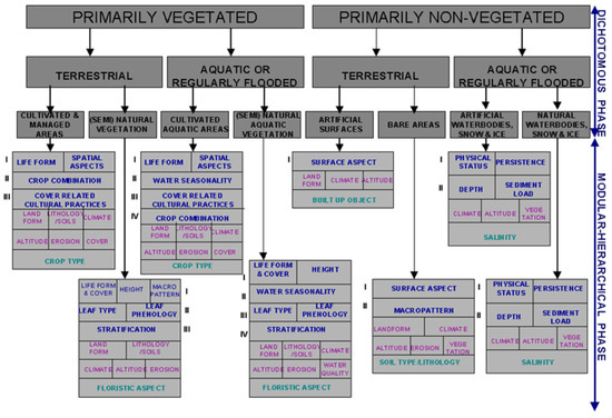
Figure 1.
As in [16], courtesy of the Food and Agriculture Organization (FAO of the United Nations (UN). Two-stage fully-nested FAO Land Cover Classification System (LCCS) taxonomy. The first-stage fully-nested 3-level 8-class FAO LCCS Dichotomous Phase (DP) taxonomy is general-purpose, user- and application-independent. It consists of a sorted set of three dichotomous layers: (i) vegetation versus non-vegetation, (ii) terrestrial versus aquatic, and (iii) managed versus natural or semi-natural. These three dichotomous layers deliver as output the following 8-class FAO LCCS-DP taxonomy. (A11) Cultivated and Managed Terrestrial (non-aquatic) Vegetated Areas. (A12) Natural and Semi-Natural Terrestrial Vegetation. (A23) Cultivated Aquatic or Regularly Flooded Vegetated Areas. (A24) Natural and Semi-Natural Aquatic or Regularly Flooded Vegetation. (B35) Artificial Surfaces and Associated Areas. (B36) Bare Areas. (B47) Artificial Waterbodies, Snow and Ice. (B48) Natural Waterbodies, Snow and Ice. The general-purpose user- and application-independent 3-level 8-class FAO LCCS-DP taxonomy is preliminary to a second-stage FAO LCCS Modular Hierarchical Phase (MHP) taxonomy, consisting of a battery of user- and application-specific one-class classifiers, equivalent to one-class grammars (syntactic classifiers) [19].
Figure 1 shows that the standard two-phase fully-nested FAO LCCS hierarchy consists of a first-stage fully-nested general-purpose, user- and application-independent 3-level 8-class FAO LCCS-DP legend, preliminary to a second-stage application-dependent and user-specific FAO LCCS Modular Hierarchical Phase (MHP) taxonomy, consisting of a hierarchical (deep) battery of one-class classifiers [16]. The standard first-stage 3-level 8-class FAO LCCS-DP hierarchy is “fully nested”. It comprises three dichotomous LC class-specific information layers, equivalent to a world ontology, world model or mental model of the real-world [13,16,19,20,21,22,23,24]: DP Level 1—Vegetation versus non-vegetation, DP Level 2—Terrestrial versus aquatic and DP Level 3—Managed versus natural or semi-natural. In recent years, the two-phase FAO LCCS taxonomy has become increasingly popular [25]. One reason for its popularity is that the FAO LCCS hierarchy is “fully nested” while alternative LC class hierarchies, such as the Coordination of Information on the Environment (CORINE) Land Cover (CLC) taxonomy [26], the U.S. Geological Survey (USGS) Land Cover Land Use (LCLU) taxonomy by J. Anderson [27], the International Global Biosphere Programme (IGBP) DISCover Data Set Land Cover Classification System [28] and the EO Image Librarian LC class legend [29], start from a Level 1 taxonomy which is already multi-class. In a hierarchical EO image understanding (EO-IU) system architecture submitted to a garbage in, garbage out (GIGO) information principle, synonym for error propagation through an information processing chain, the fully-nested two-phase FAO LCCS hierarchy makes explicit the full dependence of high-level LC class estimates, performed by any high-level (deep) LCCS-MHP data processing module, on the operational quality (in accuracy, efficiency, robustness, etc.) of lower-level LCCS modules, starting from the initial FAO LCCS-DP Level 1 vegetation/non-vegetation information layer whose relevance in thematic mapping accuracy (vice versa, in error propagation) becomes paramount for all subsequent LCCS layers.
The GIGO commonsense principle, intuitive to understand in general terms as error propagation through an information processing chain, becomes neither trivial nor obvious to understand when applied to a hierarchical LC class taxonomy, starting from a FAO LCCS-DP Level 1 vegetation/non-vegetation and featuring inter-layer semantic dependencies, equivalent to transmission lines where semantic error can propagate, from low-level (coarse) to high-level (fine) semantics [30]. On the one hand, an inherently difficult image classification scenario into vegetated/non-vegetated LC classes agrees with a minor portion of the RS literature where supervised data learning classification of EO image datasets at continental or global spatial extent into binary LC class vegetation/non-vegetation is considered very challenging [31]. On the other hand, it is at odd with the RS mainstream, where the semantic information gap from sub-symbolic EO data to multi-class LC taxonomies, where target LC classes are far deeper in semantics than the initial FAO LCCS-DP Level 1 vegetation/non-vegetation information layer, is typically filled in one conceptual stage, highly informative, but opaque (mysterious, unfathomable) in nature. This one-stage mapping from sub-symbolic sensory data to high-level (symbolic) concepts is typically implemented as a supervised data learning classification stage [32,33], e.g., a support vector machine, random forest or deep convolutional neural network (DCNN) [34,35,36,37,38], which is equivalent to a black box learned from supervised (labeled) data based on heuristics (e.g., architectural metaparameters are typically user-defined by trial-and-error) [30], whose opacity contradicts the well-known engineering principles of modularity, regularity and hierarchy typical of scalable systems [39]. In addition, inductive algorithms, capable of learning from either supervised (labeled) or unsupervised (unlabeled) data, are inherently semi-automatic and site-specific [2]. In general, "No Free Lunch” theorems have shown that inductive learning-from-data algorithms cannot be universally good [40,41].
Over land surfaces of the Earth, the global cloud cover is approximately 66% [42]. In the ESA EO Level 2 product definition, cloud and cloud–shadow quality layer requirements specification accounts for a well-known prerequisite of clear-sky multi-temporal EO image compositing and understanding (classification) solutions proposed by the RS community, where accurate masking of cloud and cloud–shadow phenomena is considered necessary, but not sufficient pre-condition [12,13,43,44,45,46,47,48,49,50,51,52,53,54,55,56,57,58,59,60,61,62,63]. Intuitively, in single-date and multi-temporal MS image analysis, cloud and cloud–shadow preliminary detection is a relevant problem, because unflagged cloud and cloud–shadow phenomena may be mapped onto erroneous LC classes or false LC change (LCC) occurrences.
It is noteworthy that joint (combined) cloud and cloud–shadow detection is a typical example of physical model-based cause–effect relationship, expected to be very difficult to solve by inductive machine learning-from-data algorithms, such as increasingly popular DCNNs [34], with special regard to DCNNs designed and trained end-to-end for semantic segmentation [37] and instance segmentation [38] tasks, whereas DCNNs trained for object detection, such as [36], where image-objects are localized with bounding boxes and categorized into one-of-many categories, are inapplicable to the cloud/cloud–shadow instance segmentation problem of interest. In general, inductive supervised data learning algorithms are capable of learning complex correlations between input and output features, but unsuitable for inherent representations of causality [30,64], in agreement with the well-known dictum that correlation does not imply causation and vice versa [13,19,30,33,64,65].
In the last decade, many different cloud/cloud–shadow detection algorithms have been presented in the RS literature to run either on a single-date MS image or on an MS image time-series, typically acquired by either one EO spaceborne/airborne MS imaging sensor or a single family (e.g., Landsat) of MS imaging sensors [12,13,43,44,45,46,47,48,49,50,51,52,53,54,55,56,57,58,59,60]. To be accomplished in operating mode at the ground segment (midstream) by EO data providers in support of the downstream sector within a “seamless chain of innovation” needed for a new era of Space Economy 4.0 [66], systematic radiometric Cal of multi-source multi-angular multi-temporal MS big image data cubes [1,3,13,67,68,69], encompassing either single-date or multi-temporal cloud and cloud–shadow detection as a necessary-but-not-sufficient pre-condition, is regarded by the RS community as an open problem to date [61,62,63].
In agreement with the GEO-CEOS QA4EO Cal/Val requirements [3], this work presents an innovative AutoCloud+ computer vision (CV) software system for cloud and cloud–shadow quality layer detection. To be eligible for systematic ESA EO Level 2 product generation at the ground segment [43,67,70], AutoCloud+ must overcome conceptual (structural) limitations and well-known failure modes of standard cloud and cloud–shadow detection algorithms [44,47,61,62,63], such as the single-date multi-sensor Function of Mask (FMask) open source algorithm [58,59], the single-date single-sensor ESA Sen2Cor software toolbox [11,12,44], to be run free-of-cost on the user side, and the multi-date Multisensor Atmospheric Correction and Cloud Screening (MACCS)-Atmospheric/Topographic Correction (ATCOR) Joint Algorithm (MAJA) developed and run by the Centre national d’études spatiales (CNES)/Centre d’Etudes Spatiales de la Biosphère (CESBIO)/Deutsches Zentrum für Luft- und Raumfahrt (German Aerospace Center, DLR) [46,47,48], which incorporates capabilities of the ATCOR commercial software toolbox [71,72,73,74].
A synonym for inherently ill-posed scene-from-image reconstruction and understanding [13,23,75,76], vision is a cognitive (information-as-data-interpretation) process [18], encompassing both biological vision and CV, where CV is subset-of artificial general intelligence (AI) [77,78,79,80,81], i.e., AI ⊃ CV, in the multi-disciplinary domain of cognitive science [18,77,78,79,80,81], see Figure 2. In vision, spatial information dominates color information [23]. This unquestionable true fact is familiar to all human beings wearing sunglasses: in perceptual terms, human panchromatic and chromatic visions are nearly as effective [13].
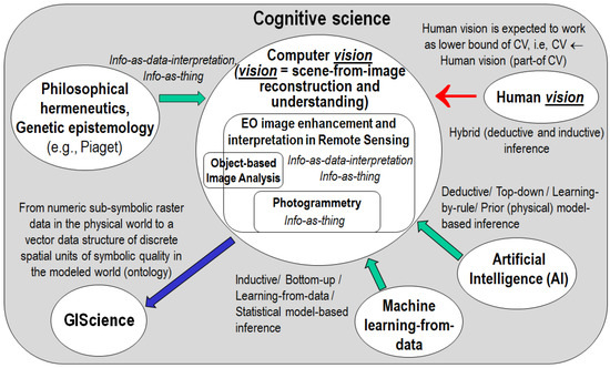
Figure 2.
Multi-disciplinary cognitive science domain, adapted from [18,77,78,79,80,81], where it is postulated that ‘Human vision → computer vision (CV)’, where symbol ‘→’ denotes relationship part-of pointing from the supplier to the client, not to be confused with relationship subset-of, ‘⊃’, meaning specialization with inheritance from the superset to the subset, in agreement with the standard Unified Modeling Language (UML) for graphical modeling of object-oriented software [86]. The working hypothesis ‘Human vision → CV’ means that human vision is expected to work as lower bound of CV, i.e., a CV system is required to include as part-of a computational model of human vision [13,76,87,88,89,90,91,92,93,94,95,96,97,98,99,100,101,102,103,104]. In practice, to become better conditioned for numerical solution, an inherently ill-posed CV system is required to comply with human visual perception phenomena in the multi-disciplinary domain of cognitive science. Cognitive science is the interdisciplinary scientific study of the mind and its processes. It examines what cognition (learning, adaptation, self-organization) is, what it does and how it works [18,77,78,79,80,81]. It especially focuses on how information/knowledge is represented, acquired, processed and transferred either in the neuro-cerebral apparatus of living organisms or in machines, e.g., computers. Like engineering, remote sensing (RS) is a meta-science [105], the goal of which is to transform knowledge of the world, provided by other scientific disciplines, into useful user- and context-dependent solutions in the world. Neuroscience, in particular neurophysiology, studies the neuro-cerebral apparatus of living organisms. Neural network (NN) is synonymous with distributed processing system, consisting of neurons as elementary processing elements and synapses as lateral connections. Is it possible and even convenient to mimic biological mental functions, e.g., human reasoning, by means of an artificial mind whose physical support is not an electronic brain implemented as an artificial NN (ANN)? The answer is no according to the “connectionists approach” promoted by traditional cybernetics, where a complex system always comprises an “artificial mind-electronic brain” combination. This is alternative to a traditional approach to artificial intelligence (AI), whose so-called symbolic approach investigates an artificial mind independently of its physical support [77].
Starting from this simple, yet not trivial, observation about human visual perception, in order to outperform standard CV software toolboxes in operating mode for cloud and cloud–shadow detection in EO big data cubes, such as the single-date sensor-specific ESA Sen2Cor [11,12,44] and the multi-date multi-sensor CESBIO/CNES/DLR MAJA software [46,47,48], degrees of novelties of an innovative “universal” AutoCloud+ CV software system are expected to encompass the Marr five levels of understanding of an information processing system, specifically [13,19,76,82,83]:
- outcome and process requirements specification, including computational complexity estimation,
- information/knowledge representation,
- system design (architecture),
- algorithm, and
- implementation.
Among these five levels, the three more abstract ones, namely, outcome and process requirements specification, information/knowledge representation and system design, are typically considered the linchpin of success of an information processing system, rather than algorithm and implementation [13,19,76,82,83].
To be considered “universal” and in operating mode, the AutoCloud+ software system’s outcome and process requirements were specified as follows.
- (i)
- “Fully automated”, i.e., no human–machine interaction and no labeled data set for supervised inductive learning-from-data are required by the system to run, which reduces timeliness, which is the time span from EO data acquisition to EO data-derived VAPS generation, as well as costs in manpower (e.g., to collect training data) and computer power (no training time is required).
- (ii)
- Near real-time, e.g., computational complexity increases linearly with image size.
- (iii)
- Robust to changes in input sensory data acquired across space, time and sensors.
- (iv)
- Scalable to changes in MS imaging sensor’s spatial and spectral resolution specifications.
- (v)
- Last but not least, AutoCloud+ must be eligible for use in multi-sensor, multi-temporal and multi-angular EO big data cubes, either radiometrically uncalibrated, such as MS images typically acquired without radiometric Cal metadata files by small satellites [84] or small unmanned aerial vehicles (UAVs) [85], or radiometrically calibrated into TOARF, SURF or surface albedo values in agreement with the GEO-CEOS QA4EO Cal/Val requirements [3].
For the sake of readability this paper is divided in two. The present Part 1 highlights why AutoCloud+ is important in a broad context of systematic ESA EO Level 2 product generation at the ground segment within a “seamless innovation chain” needed for a new era of Space 4.0 [66]. Heavily referenced, this in-depth problem background discussion can be skipped by expert readers. In the subsequent Part 2 (see Supplementary Materials), first, a “universal” AutoCloud+ CV software system is instantiated at the Marr five levels of understanding of an information processing system (refer to this Section above) [13,19,76,82,83]. Second, preliminary experimental results, collected from an AutoCloud+ prototypical implementation and integration, are presented and discussed.
The rest of the present Part 1 is organized as follows. Section 2 critically reviews the cognitive (information-as-data-interpretation) problem of systematic ESA EO Level 2 product generation, whose necessary-but-not-sufficient pre-condition is cloud and cloud–shadow quality layers detection. Section 3 surveys standard algorithms for cloud and cloud–shadow quality layers detection, available either open source or free-of-cost. Conclusions are reported in Section 4.
2. Systematic ESA EO Level 2 Information Product Generation as a Broad Context of Cloud/Cloud–Shadow Quality Layers Detection in a Cognitive Science Domain
Systematic ESA EO Level 2 product generation at the ground segment in multi-source EO big data cubes [11,12] is an inherently ill-posed CV problem [13,23,75,76]; the necessary-but-not-sufficient pre-condition of this CV problem is the inherently ill-posed CV sub-problem of cloud and cloud–shadow quality layers detection. The former is regarded as a broad context where the importance and degree of complexity of the latter are highlighted.
Featuring a relevant survey value in the multidisciplinary domain of cognitive science [18,77,78,79,80,81], encompassing AI ⊃ CV (see Figure 2), this section provides a critical review of ESA EO Level 2 product generation strategies. Expert readers non-interested in the broad context of cloud and cloud shadow quality layers detection can skip this review section and move directly to either Section 3 in the present Part 1 or the Part 2 (proposed as Supplementary Materials) of this paper.
In this review section, the Marr two lower levels of abstraction of an information processing system, identified as algorithm and implementation (see Section 1), are ignored. Rather, it focuses on the Marr (three more abstract) levels of understanding known as outcome and process requirements specification, information/knowledge representation and system design (see Section 1), because they are typically considered the cornerstone of success of an information processing system [13,19,76,82,83]. Hence, this critical review is not alternative, but complementary to surveys on EO image understanding systems typically proposed in the RS literature, such as [6,7,8], focused exclusively on the two lower levels of abstraction, specifically, algorithm and implementation. In more detail, among the three aforementioned surveys, EO image preprocessing requirements, such as radiometric Cal, atmospheric correction and topographic correction, although considered mandatory by the GEO-CEOS QA4EO Cal/Val guidelines [3], are totally ignored in surveys [6,7], published in year 2014 and 2016 respectively. In contrast, EO image pre-processing issues are briefly taken into account by the third survey [8], dating back to year 2007. This observation supports the thesis that, in more recent years, when computational power has been exponentially increasing according to the Moore law of productivity [106], statistical model-based (inductive) image analysis algorithms have been dominating the RS literature, whereas physical model-based or hybrid (combined statistical and physical model-based) inference algorithms, which require as input sensory data provided with a physical meaning, specifically, EO data provided with a physical unit of radiometric measure in agreement with the GEO-CEOS QA4EO Cal/Val requirements [3], have been increasingly oversighted.
To successfully cope with the five Vs of EO big data analytics, specifically, volume, variety, veracity, velocity and value [4], multi-sensor analysis of multi-temporal multi-angular EO sensory data cubes depends upon the ability to distinguish between relevant changes and no-changes occurring at the Earth surface through time [68,69]. A necessary-but-not-sufficient pre-condition for EO big data transformation into timely, comprehensive and operational EO data-derived VAPS, expected by GEO to be pursued by a GEOSS never accomplished to date [5], is radiometric Cal, considered mandatory by the GEO-CEOS QA4EO Cal/Val requirements [3], but largely oversighted in the RS common practice and literature, e.g., see [6,7]. In short, radiometric Cal guarantees EO sensory data interoperability (consistency, harmonization, reconciliation, “normalization”) across time, geographic space and sensors. In greater detail, the capability to detect and quantify change/no-change in terms of either qualitative (nominal, categorical) Earth surface variables, such as LC classes belonging to a finite and discrete LC class taxonomy (legend), or quantitative (numeric) Earth surface variables, such as biophysical variables, e.g., leaf area index (LAI), biomass, etc., depends on the radiometric Cal of EO sensory data, equivalent to non-negative dimensionless DNs ≥ 0, provided with no physical meaning and typically affected at sensor-level by ever-varying atmospheric conditions, solar illumination conditions, spaceborne/airborne viewing geometries and Earth surface topography, into a physical variable provided with a community-agreed radiometric unit of measure, such as TOARF, SURF or surface albedo values in range 0.0–1.0 [1,2,3]. Solar illumination conditions are typically parameterized by metadata Cal parameters, such as image acquisition time, solar exo-atmospheric irradiance, solar zenith angle and solar azimuth angle, see Figure 3. Sensor viewing characteristics are typical metadata Cal parameters, such as sensor zenith angle and sensor azimuth angle, see Figure 3. Atmospheric conditions are described by categorical variables, such as aerosol type, haze, cloud and cloud–shadow, and by numeric variables, such as water vapor, temperature and aerosol optical thickness (AOT) [68,69]. Finally, Earth surface geometries must be inferred from ancillary data, such as a digital elevation model (DEM), in combination with solar and viewing conditions [107], see Figure 3.
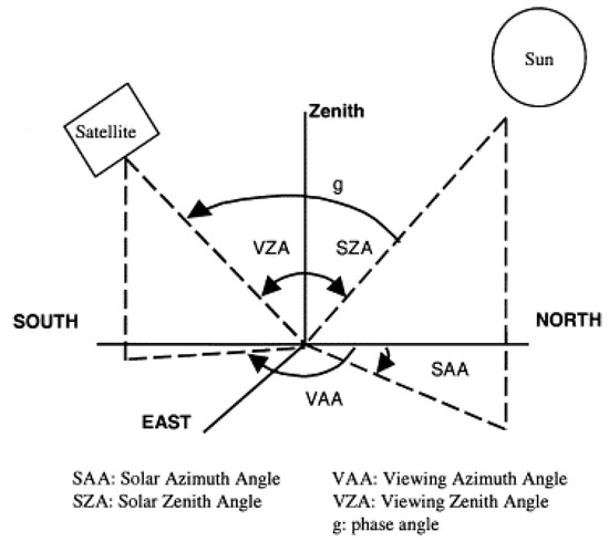
Figure 3.
Solar illumination geometries and viewpoint geometries in spaceborne and airborne EO image acquisition.
Adopted by different scientific disciplines, such as inductive machine learning-from-data [32,33], AI as superset-of CV [77], i.e., AI ⊃ CV (see Figure 2), and RS [2,13], popular synonyms for deductive inference are top-down inference, prior knowledge-based inference, learning-by-rule inference and physical model-based inference. Synonyms for inductive inference are bottom-up inference, learning-from-data inference, learning-from-examples inference and statistical model-based inference [82,83].
On the one hand, non-calibrated sensory data, provided with no physical meaning, can be investigated by statistical data models and inductive inference algorithms, exclusively. On the other hand, although they do not require physical variables as input, statistical data models and inductive learning-from-data algorithms can benefit from input data Cal in terms of augmented robustness to changes in the input data set acquired through time, space and sensors. In contrast, radiometrically calibrated data, provided with a physical meaning, can be interpreted by either inductive, deductive (physical model-based) or hybrid (combined deductive and inductive) inference algorithms. Although it is considered a well-known “prerequisite for physical model-based (and hybrid) analysis of airborne and satellite sensor measurements in the optical domain” [1,13,67,68,69], EO data Cal is largely neglected in the RS common practice. For example, in major portions of the RS literature, including the GEOBIA sub-domain of GIScience [9,10], no reference to radiometric Cal issues is found. This lack of input EO data Cal requirements proves that, to date, EO image analytics mainly consists of inductive learning-from-data algorithms, starting from scratch because no a priori physical knowledge is exploited in addition to data. This is in contrast with biological cognitive systems, where “there is never an absolute beginning” [108], because a priori genotype provides initial conditions (that reflect properties of the world, embodied through evolution, based on evolutionary experience) to learning-from-examples phenotype, according to a hybrid inference paradigm, where phenotype explores the neighborhood of genotype in a solution space [13,78]. Hybrid inference combines deductive and inductive inference to take advantage of each and overcome their shortcomings [2]. Inductive inference is typically semi-automatic and site-specific [2]. Deductive inference is static (non-adaptive to data) and typically lacks flexibility to transform ever-varying sensory data (sensations) into stable percepts (concepts) in a world model [13,23,82,83].
In compliance with the GEO-CEOS QA4EO Cal/Val requirements and the visionary goal of a GEOSS [5], ESA has recently provided an original ESA EO Level 2 information product definition, refer to Section 1 [11,12]. The ESA EO Level 2 product definition is non-trivial. Notably, it is more restrictive than the National Aeronautics and Space Administration (NASA) EO Level 2 product definition of “a data-derived geophysical variable at the same resolution and location as Level 1 source data” [109]. According to the standard Unified Modeling Language (UML) for graphical modeling of object-oriented software [86], where symbol ‘→’ denotes relationship part-of pointing from the supplier to the client (vice versa, it would denote relationship depend-on), not to be confused with relationship subset-of, whose symbol is ‘⊃’, meaning specialization with inheritance from the superset to the subset, the following dependence relationship holds true:
Depicted in Figure 4, this dependence relationship implies that a NASA EO Level 2 product can be accomplished although no ESA EO Level 2 product exists, whereas the vice versa does not hold.
‘NASA EO Level 2 product → ESA EO Level 2 product’.
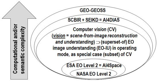
Figure 4.
In agreement with the standard Unified Modeling Language (UML) for graphical modeling of object-oriented software [86], relationship part-of, denoted with symbol ‘→’ pointing from the supplier to the client, should not to be confused with relationship subset-of, ‘⊃’, meaning specialization with inheritance from the superset to the subset. A National Aeronautics and Space Administration (NASA) EO Level 2 product is defined as “a data-derived geophysical variable at the same resolution and location as Level 1 source data” [109]. Herein, it is considered part-of an ESA EO Level 2 product defined as [11,12]: (a) a single-date multi-spectral (MS) image whose digital numbers (DNs) are radiometrically corrected into surface reflectance (SURF) values for atmospheric, adjacency and topographic effects, stacked with (b) its data-derived general-purpose, user- and application-independent scene classification map (SCM), whose thematic map legend includes quality layers cloud and cloud–shadow. In this paper, ESA EO Level 2 product is regarded as an information primitive to be accomplished by Artificial Intelligence for the Space segment (AI4Space), such as in future intelligent small satellite constellations, rather than at the ground segment in an AI for data and information access services (AI4DIAS) framework. In this graphical representation, additional acronyms of interest are computer vision (CV), whose special case is EO image understanding (EO-IU) in operating mode, semantic content-based image retrieval (SCBIR) [13,110,111,112,113,114,115], semantics-enabled information/knowledge discovery (SEIKD), where SCIR + SEIKD is considered synonym for AI4DIAS, and Global Earth Observation System of Systems (GEOSS), defined by the Group on Earth Observations [5]. Our working hypothesis postulates that the following dependence relationship holds true. ‘NASA EO Level 2 product → ESA EO Level 2 product = AI4Space ⊂ EO-IU in operating mode ⊂ CV → [EO-SCBIR + SEIKD = AI4DIAS] → GEO-GEOSS’. This equation means that GEOSS, whose part-of are the still-unsolved (open) problems of SCBIR and SEIKD, cannot be achieved until the necessary-but-not-sufficient pre-condition of CV in operating mode, specifically, systematic ESA EO Level 2 product generation, is accomplished in advance. Encompassing both biological vision and CV, vision is synonym for scene-from-image reconstruction and understanding. Vision is a cognitive (information-as-data-interpretation) problem [18] very difficult to solve because: (i) non-deterministic polynomial (NP)-hard in computational complexity [87,116], (ii) inherently ill-posed in the Hadamard sense [23,75,117], because affected by: (I) a 4D-to-2D data dimensionality reduction from the 4D geospatial-temporal scene-domain to the (2D, planar) image-domain, e.g., responsible of occlusion phenomena, and (II) a semantic information gap from ever-varying sub-symbolic sensory data (sensations) in the physical world to stable symbolic percepts in the mental model of the physical world (modeled world, world ontology, real-world model) [13,18,19,20,21,22,23,24]. Since it is inherently ill-posed, vision requires a priori knowledge in addition to sensory data to become better posed for numerical solution [32,33]. If the aforementioned working hypothesis holds true, then the complexity of SCBIR + SEIKD is not inferior to the complexity of vision, acknowledged to be inherently ill-posed and NP-hard. To make the inherently-ill-posed CV problem better conditioned for numerical solution, a CV system is required to comply with human visual perception. In other words, a CV system is constrained to include a computational model of human vision [13,76,87,88,89,90,91,92,93,94,95,96,97,98,99,100,101,102,103,104], i.e., ‘Human vision → CV’. Hence, dependence relationship: ‘Human vision → CV ⊃ EO-IU in operating mode ⊃ NASA EO Level 2 product → ESA EO Level 2 product → [EO-SCBIR + SEIKD = AI4DIAS] → GEO-GEOSS’ becomes our working hypothesis (to be duplicated in the body text). Equivalent to a first principle (axiom, postulate), This equation can be considered the first original contribution, conceptual in nature, of this research and technological development (RTD) study.
An improved (“augmented”) and more restrictive ESA EO Level 2 product definition could be defined to account for bidirectional reflectance distribution function (BRDF) effect correction, in addition to atmospheric, topographic and adjacency effects correction, to model surface anisotropy in multi-temporal multi-angular EO image data cubes [2,68,69,74,118,119,120,121]. A surface that reflects the incident energy equally in all directions is said to be Lambertian, where reflectance is invariant with respect to illumination and viewing conditions, see Figure 3. On the contrary, a surface is said to be anisotropic when its reflectance varies with respect to illumination and/or viewing geometries. These changes are driven by the optical and structural properties of the surface material. In other words, in EO image pre-processing (enhancement) for radiometric Cal, BRDF effect correction is LC class-specific [68,69,74,118,119,120,121]. The LC class-specific task of BRDF correction is to derive, for non-Lambertian surfaces, spectral albedo (bi-hemispherical reflectance, BHR) values, defined over all directions [2,74,118,119,120,121], from either SURF or TOARF values where the Lambertian surface assumption holds [71,72,73,74,118].
Our working hypothesis, depicted in Figure 4, when translated into symbols of the standard UML for graphical modeling of object-oriented software [86] can be formulated as follows (refer to the caption of Figure 4):
Duplicated from the caption of Figure 4 and regarded as the first original contribution of this research and technological development (RTD) study, Equation (1) shows our working hypothesis as dependence relationship, equivalent to a first principle (axiom, postulate). In more detail, Equation (1) postulates that systematic ESA EO Level 2 product generation is an inherently ill-posed CV problem, where CV ⊃ EO-IU, whose solution in operating mode is necessary-but-not-sufficient pre-condition for the yet-unaccomplished dependent problems of semantic content-based image retrieval (SCBIR) [13,110,111,112,113,114,115] and semantics-enabled information/knowledge discovery (SEIKD) in large-scale EO image data cubes, with SCBIR + SEIKD considered synonym for AI for Data and Information Access Services (AI4DIAS), where AI4DIAS is part-of a yet-unaccomplished GEOSS. The closed-loop AI4DIAS system architecture, suitable for semantics-enabled incremental learning [13,115], is sketched in Figure 5 [13].
‘Human vision → CV ⊃ EO-IU in operating mode ⊃ NASA EO Level 2 product → ESA EO Level 2 product → [EO-SCBIR + SEIKD = AI4DIAS] → GEO-GEOSS’.
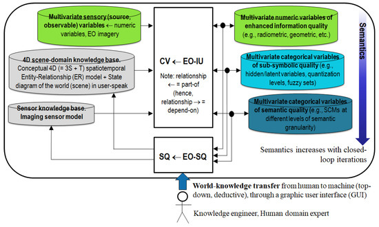
Figure 5.
Artificial intelligence (AI) for Data and Information Access Services (AI4DIAS), synonym for semantics-enabled DIAS or closed-loop EO image understanding (EO-IU) for semantic querying (EO-IU4SQ) system architecture. At the Marr level of system understanding known as system design (architecture) [76], AI4DIAS is sketched as a closed-loop EO-IU4SQ system architecture, suitable for incremental semantic learning. It comprises a primary (dominant, necessary-but-not-sufficient) hybrid (combined deductive and inductive) feedback (provided with feedback loops) EO-IU subsystem in closed-loop with a secondary (dominated) hybrid feedback EO-SQ subsystem. Subset-of a computer vision (CV) system, where CV ⊃ EO-IU, the EO-IU subsystem is required to be automatic (no human–machine interaction is required by the CV system to run) and near real-time to provide the EO-SQ subsystem with useful information products, including thematic maps of symbolic quality, such as single-date ESA EO Level 2 Scene Classification Map (SCM) considered a necessary-but-not-sufficient pre-condition to semantic querying, synonym for semantics-enabled information/knowledge discovery (SEIKD) in massive multi-source EO image databases. The EO-SQ subsystem is provided with a graphic user interface (GUI) to streamline: (i) top-down knowledge transfer from-human-to-machine of an a priori mental model of the 4D geospatial-temporal real-world, (ii) high-level user- and application-specific EO semantic content-based image retrieval (SCBIR) operations. Output products generated by the closed-loop EO-IU4SQ system are expected to monotonically increase their value-added with closed-loop iterations, according to Bayesian updating where Bayesian inference is applied iteratively [122,123]: after observing some evidence, the resulting posterior probability can be treated as a prior probability and a new posterior probability computed from new evidence. One of Marr’s legacies is the notion of computational constraints required to make the typically ill-posed non-deterministic polynomial (NP)-hard problem of intelligence, encompassing vision [87], better conditioned for numerical solution [32,33]. Marr’s computational constraints reflecting properties of the world are embodied through evolution, equivalent to genotype [78], into the human visual complex system, structured as a hierarchical network of networks with feedback loops [87,88,89,90,91,92,93,96,97,98]. Marr’s computational constraints are Bayesian priors in a Bayesian inference approach to vision [76,122], where ever-varying sensations (sensory data) are transformed into stable percepts (concepts) about the world in a world model [23], to perform successfully in the world [18].
The working hypothesis (1) regards the ESA EO Level 2 information product as baseline information unit (information primitive) whose systematic generation is of paramount importance to contribute toward filling an analytic and pragmatic information gap from multi-sensor, multi-temporal and multi-angular EO big image data cubes into timely, comprehensive and operational EO data-derived VAPS, in compliance with the visionary goal of a GEOSS [3,5], unaccomplished to date. To justify our working hypothesis (1), let us introduce, first, the definition proposed for an EO-IU system to be considered in operating mode and, second, the background knowledge of vision stemming from the multidisciplinary domain of cognitive science [18,77,78,79,80,81].
Based on scientific literature [13,14,15,67,82,83,124], a CV ⊃ EO-IU system is defined in operating mode if and only if it scores “high” in every index of a minimally dependent and maximally informative (mDMI) set of EO outcome and process (OP) quantitative quality indicators (Q2Is), to be community-agreed upon for use by members of the RS community, in agreement with the GEO-CEOS QA4EO Cal/Val guidelines [3]. A proposed instantiation of an mDMI set of EO OP-Q2Is includes the following.
- (i)
- Degree of automation, inversely related to human–machine interaction, e.g., inversely related to the number of system’s free-parameters to be user-defined based on heuristics.
- (ii)
- Effectiveness, e.g., thematic mapping accuracy.
- (iii)
- Efficiency in computation time and in run-time memory occupation.
- (iv)
- Robustness (vice versa, sensitivity) to changes in input data.
- (v)
- Robustness to changes in input parameters to be user-defined.
- (vi)
- Scalability to changes in user requirements and in sensor specifications.
- (vii)
- Timeliness from data acquisition to information product generation.
- (viii)
- Costs in manpower and computer power.
- (ix)
- Value, e.g., semantic value of output products, economic value of output services, etc.
According to the Pareto formal analysis of multi-objective optimization problems, optimization of an mDMI set of OP-Q2Is is an inherently-ill posed problem in the Hadamard sense [117], where many Pareto optimal solutions lying on the Pareto efficient frontier can be considered equally good [125]. Any EO-IU system solution lying on the Pareto efficient frontier can be considered in operating mode, therefore suitable to cope with the five Vs of spatial-temporal EO big data, namely, volume, variety, veracity, velocity and value [4].
In the multidisciplinary domain of cognitive science (see Figure 2), vision is synonym for scene-from-image reconstruction and understanding [23], see Figure 6. Encompassing both biological vision and CV, vision is a cognitive (information-as-data-interpretation) problem [18], very difficult to solve because: (i) non-deterministic polynomial (NP)-hard in computational complexity [87,116], (ii) inherently ill-posed in the Hadamard sense [117], i.e., vision admits no solution, multiple solutions or, if the solution exists, the solution’s behavior changes continuously with the initial conditions [23,75]. Vision is inherently ill-posed because affected by: (I) a 4D-to-2D data dimensionality reduction, from the geospatial-temporal scene-domain to the (2D, planar) image-domain, e.g., responsible of occlusion phenomena, and (II) a semantic information gap, from ever-varying sub-symbolic sensory data (sensations) in the physical world to stable symbolic percepts in the mental model of the physical world (modeled world, world ontology, real-world model) [12,18,19,20,21,22,23,24], see Figure 6. Since it is inherently ill-posed, vision requires a priori knowledge in addition to sensory data to become better posed for numerical solution [32,33]. For example, in inherently ill-posed CV systems, a valuable source of a priori knowledge is reverse engineering primate visual perception [87,88,89,90,91,92,93], so that a CV system is constrained to include a computational model of human vision [13,76,87,88,89,90,91,92,93,94,95,96,97,98,99,100,101,102,103,104], i.e., ‘Human vision → CV’, see Figure 2. According to cognitive science, AI ⊃ CV is not a problem in statistics [125], which is tantamount to saying there is no (qualitative, equivocal, nominal) semantics in (quantitative, unequivocal, numeric) sensory data [13]. These principles are implicit in the dual meaning of the word “information”, either quantitative (unequivocal) information-as-thing, typical of the Shannon data communication/transmission theory [126], or qualitative (equivocal) information-as-data-interpretation, typical of AI ⊃ CV tasks investigated by philosophical hermeneutics [18].
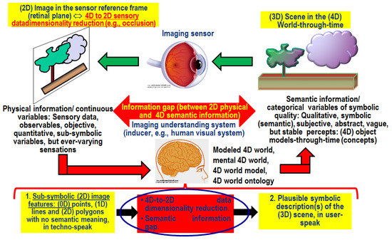
Figure 6.
Synonym for scene-from-image reconstruction and understanding, vision is a cognitive (information-as-data-interpretation) problem [18] very difficult to solve because: (i) non-deterministic polynomial (NP)-hard in computational complexity [87,116], and (ii) inherently ill-posed [23,75] in the Hadamard sense [117]. Vision is inherently ill-posed because affected by: (I) a 4D-to-2D data dimensionality reduction from the 4D geospatial-temporal scene-domain to the (2D, planar) image-domain, e.g., responsible of occlusion phenomena, and (II) a semantic information gap from ever-varying sub-symbolic sensory data (sensations) in the physical world-domain to stable symbolic percepts in the mental model of the physical world (modeled world, world ontology, real-world model) [13,18,19,20,21,22,23,24]. Since it is inherently ill-posed, vision requires a priori knowledge in addition to sensory data to become better posed for numerical solution [32,33].
Largely oversighted by the RS and CV literature, an undisputable observation (true-fact) is that, in general, spatial information dominates color information in vision [23]. This commonsense knowledge is obvious, but not trivial. On the one hand, it may sound awkward to many readers, including RS experts and CV practitioners. On the other hand, it is acknowledged implicitly by all human beings wearing sunglasses: human panchromatic vision is nearly as effective as chromatic vision in scene-from-image reconstruction and understanding [13]. This true fact means that spatial information dominates both the 4D geospatial-temporal scene-domain and the (2D) image-domain involved with the cognitive task of vision, see Figure 6. This evidence is also acknowledged by the Tobler’s first law (TFL) of geography, familiar to geographers working in the real-world domain. The TFL of geography states that “all things are related, but nearby things are more related than distant things” [127], although certain phenomena clearly constitute exceptions [128]. Obscure to many geographers familiar with the TFL formulation, the statistical concept of spatial autocorrelation is the quantitative counterpart of the qualitative TFL of geography [13]. The relevance of spatial autocorrelation in both the 4D geospatial-temporal scene-domain and the (2D) image domain involved with vision is at the very foundation of the (GE)OBIA approach to CV, originally conceived around year 2000 by the GIScience community as a viable alternative to traditional 1D spatial-context insensitive (pixel-based) image analysis [9,10]. Unfortunately, rather than starting with background knowledge in the multi-disciplinary domain of cognitive science, the GEOBIA approach was started from scratch by a self-referencing GEOBIA sub-community within the GIScience domain, see Figure 2 [9,10,129,130]. As a consequence of its lack of interdisciplinarity, the GEOBIA community showed an increasing tendency to “re-invent the wheel” in ever-varying implementations of the same sub-optimal EO-IU system architecture, although the CV ⊂ AI communities clearly acknowledge that the key of success of an information processing system lies on outcome and process requirements specification, information/knowledge representation and system design, rather than algorithm or implementation (refer to Section 1) [13,19,76,82,83]. Based on these observations, to enforce a ‘Human vision → CV’ paradigm, see Figure 2, the following original constraint can be adopted to make an inherently ill-posed CV system better conditioned for numerical solution [13].
If a chromatic CV ⊃ EO-IU system does not down-scale seamlessly to achromatic image analysis, then it tends to ignore the paramount spatial information in favor of subordinate (secondary) spatial context-insensitive color information, such as MS signatures typically investigated in traditional pixel-based single-date or multi-temporal EO-IU algorithms. In other words, a necessary and sufficient condition for a CV ⊃ EO-IU system to fully exploit primary spatial topological information (e.g., adjacency, inclusion, etc.) and spatial non-topological information (e.g., spatial distance, angle distance) components, in addition to secondary colorimetric information, is to perform nearly as well when input with either panchromatic or color imagery.[13]
Underpinned by this background knowledge about the cognitive process of vision, an undisputable true fact is that ESA EO Level 2 product generation is an inherently ill-posed CV problem (chicken-and-egg dilemma), whose inherently ill-posed CV sub-problem is cloud and cloud–shadow quality layers detection. Since it is inherently ill-posed, ESA EO Level 2 information product generation is, first, very difficult to solve; in fact, no ESA EO Level 2 product has ever been accomplished in an operating mode by any EO data provider at the ground segment to date. Second, it requires a priori knowledge in addition to sensory data to become better conditioned for numerical solution [32,33].
Our conclusion is that systematic ESA EO Level 2 product generation, at the core of the present work, is of potential interest to relevant portions of the RS community, involved with EO big data transformation into timely, comprehensive and operational EO data-derived VAPS [3,5]. Regarded as necessary-but-not-sufficient pre-condition for a GEOSS to cope with the five Vs of EO big data analytics, see Figure 4, systematic ESA EO Level 2 product generation is still open for solution in operating mode.
As the second original contribution of this review section, the several degrees of novelty of the ESA EO Level 2 product definition (refer to Section 1) are described below.
First, the ESA EO Level 2 product definition is innovative because it overtakes the traditional concept of EO data cube with an innovative EO data cube stacked with its data-derived value-adding information cube, synonym for semantics-enabled EO data cube or AI4DIAS, see Figure 7. A semantics-enabled EO data cube is alternative to existing EO data cubes, affected by the so-called data-rich information-poor (DRIP) syndrome [135], such as the existing first generation of the European Commission (EC) Data and Information Access Services (DIAS) [136,137]. Intuitively, EC-DIAS is affected by the DRIP syndrome because it is provided with no CV system in operating mode as inference engine, capable of transforming geospatial-temporal EO big data, characterized by the five Vs of volume, variety, veracity, velocity and value [4], into VAPS, starting from semantic information products, such as the ESA EO Level 2 SCM baseline product. Sketched in Figure 5, AI4DIAS complies with the Marr’s intuition that “vision goes symbolic almost immediately without loss of information” [76] (p. 343).
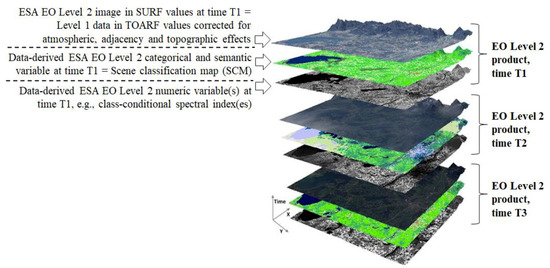
Figure 7.
Semantics-enabled EO big data cube, synonym for artificial intelligence (AI) for Data and Information Access Services (AI4DIAS). Each single-date EO Level 1 source image, radiometrically calibrated into top-of-atmosphere reflectance (TOARF) values and stored in the database, is automatically transformed into an ESA EO Level 2 product comprising: (i) a single-date multi-spectral (MS) image radiometrically calibrated from TOARF into surface reflectance (SURF) values, corrected for atmospheric, adjacency and topographic effects, stacked with (ii) its EO data-derived value-adding scene classification map (SCM), equivalent to a sensory data-derived categorical/nominal/qualitative variable of semantic quality, where the thematic map legend is general-purpose, user- and application-independent and comprises quality layers, such as cloud and cloud–shadow. It is eventually stacked with (iii) its EO data-derived value-adding numeric variables, such as biophysical variables, e.g., leaf area index (LAI) [2,131], class-conditional spectral indexes, e.g., vegetation class-conditional greenness index [132,133], categorical variables of sub-symbolic quality (geographic field-objects), e.g., fuzzy sets/discretization levels low/medium/high of a numeric variable, etc. [134].
Second, in our understanding the ESA EO Level 2 product definition is the new standard of EO Analysis Ready Data (ARD) format. This ARD definition is in contrast with the Committee on Earth Observation Satellites (CEOS) ARD for Land (CARD4L) product definition [138], where atmospheric effect removal is required exclusively, i.e., adjacency topographic and BRDF effect corrections are oversighted, and no EO data-derived SCM is expected as additional output product, which includes quality layers cloud and cloud–shadow. It is also in contrast with the U.S. Landsat ARD format [139,140,141,142,143], where atmospheric effect removal is required exclusively, i.e., adjacency topographic and BRDF effect corrections are omitted, and where quality layers cloud and cloud–shadow are required, but no EO data-derived SCM is provided as any additional output product. Finally, it is in contrast with the NASA Harmonized Landsat/Sentinel-2 (HLS) Project [142,143] where, first, atmospheric and BRDF effect corrections are required, but adjacency and topographic effect corrections are omitted, and, second, quality layers cloud and cloud–shadow are required, but no EO data-derived SCM is generated as additional output product. In practice, the CARD4L and U.S. Landsat ARD definitions are part-of the ESA EO Level 2 product definition. The latter encapsulates the former. When the latter is accomplished, so is the former; however, the vice versa does not hold.
Third, we consider ESA EO Level 2 product generation a horizontal policy for background developments in support of a new era of Space Economy 4.0 [66], see Figure 8. In the notion of Space 4.0, global value chains will require both vertical and horizontal policies. Vertical policies are more directional and ‘active’, focusing on directing change, often through mission-oriented policies that require the active creation and shaping of markets. Horizontal policies are more focused on the background conditions necessary for innovation, correcting for different types of market and system failures [66].
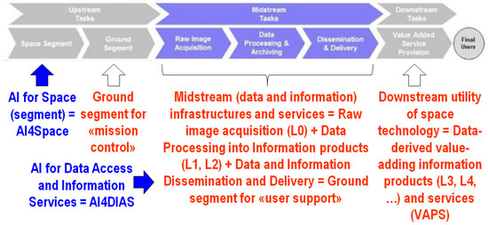
Figure 8.
Definitions adopted in the notion of Space Economy 4.0: space segment, ground segment for «mission control» = upstream, ground segment for «user support» = midstream (infrastructures and services), downstream utility of space technology [66] (pp. 6, 57). Cable of transforming quantitative (unequivocal) big data into qualitative (equivocal) data-derived value-adding information and knowledge, AI technologies should be applied as early as possible to the “seamless innovation chain” needed for a new era of Space 4.0, starting from AI4Space applications at the space segment, which include the notion of future intelligent EO satellites (FIEOS) [144,145], and AI4DIAS applications at midstream, such as systematic ESA EO Level 2 product generation, considered synonym for Analysis Ready Data (ARD) eligible for use at downstream.
Fourth, in an “old” mission-oriented (vertical) space economy [66], the ground segment is typically divided into upstream and midstream, which are defined as the portion of ground segment for mission support and user support respectively, see Figure 8. ESA expects systematic ESA EO Level 2 product generation to be accomplished by EO data providers at midstream. Actually, systematic ESA EO Level 2 product generation should occur as early as possible in the information processing chain, e.g., in the space segment preliminary to the ground segment, in compliance with the Marr’s intuition that “vision goes symbolic almost immediatel without loss of information” [76] (p. 343). Hence, in Figure 4, ESA EO Level 2 product generation becomes synonym for AI applications for the space segment, AI4Space, where AI ⊃ CV. AI4Space comes before the application of AI techniques to the ground segment, specifically, AI4DIAS. If a CV ⊂ AI application in operating mode is implemented on-board a spaceborne platform of an EO imaging sensor to provide imagery with intelligence (semantics), then Future Intelligent EO imaging Satellites (FIEOS), conceived in the early 2000s [144], become realistic, such as future intelligent EO small satellite constellations. In EO small satellite constellations provided with no on-board radiometric Cal subsystem, improved time resolution is counterbalanced by inferior radiometric Cal capabilities, considered mandatory by the GEO-CEOS QA4EO Cal/Val guidelines [3] to guarantee interoperability of multiple platforms and sensors within and across constellations. The visionary goal of AI4Space is realistic, based on the recent announcement of an RTD project focused on future intelligent small satellite constellations. The quote is: “an Earth-i led consortium will develop a number of new Earth Observation technologies that will enable processes, such as the enhancement of image resolution, cloud-detection, change detection and video compression, to take place on-board a small satellite rather than on the ground. This will accelerate the delivery of high-quality images, video and information-rich analytics to end-users. On-board cloud detection will make the tasking of satellites more efficient and increase the probability of capturing a usable and useful image or video. To achieve these goals, ‘Project OVERPaSS‘ will implement, test and demonstrate very high-resolution optical image analysis techniques, involving both new software and dedicated hardware installed on-board small satellites to radically increase their ability to process data in space. The project will also determine the extent to which these capabilities could be routinely deployed on-board British optical imaging satellites in the future” [145].
Fifth, in the RS common practice, the potential impact of the ESA EO Level 2 product definition is relevant because it makes explicit, once and for all, the undisputable true fact that atmospheric effect correction [12,56,68,69,71,72,73,74,146], adjacency and topographic effect corrections [107,147,148,149,150,151], BRDF effect correction [68,69,74,118,119,120,121], in addition to cloud/cloud shadow quality layer detection [12,13,43,44,45,46,47,48,49,50,51,52,53,54,55,56,57,58,59,60,61,62,63], are inherently ill-posed CV problems [23,75] in the Hadamard sense [117], whose solution does not exist or, if it exists, it is not unique or it is not robust to small changes in the initial condition, including changes to the input dataset. Since they are inherently ill-posed, atmospheric, topographic, adjacency and BRDF effect corrections, in addition to cloud/cloud shadow quality layer mapping, require a priori knowledge in addition to sensory data to become better posed for numerical solution [32,33]. This is tantamount to saying that radiometric Cal of EO imagery, encompassing ESA EO Level 2 product generation, is a chicken-and-egg dilemma [13,147]. On the one hand, no EO image understanding (classification) into a finite and discrete taxonomy of LC classes, in addition to categorical layers cloud and cloud–shadow, is possible in operating mode if radiometric Cal is not accomplished in advance, where dimensionless DNs are transformed into a physical unit of radiometric measure to guarantee data interoperability through space, time and sensors, in agreement with the GEO QA4EO Cal/Val requirements [5]. On the other hand, no radiometric Cal of EO imagery is possible without knowing in advance LC classes and nominal quality layers, such as cloud and cloud–shadow masks, since atmospheric, topographic and BRDF effect corrections are LC class-dependent. This is tantamount to saying that, to become better posed for automatic numerical solution (requiring no human–machine interaction), an inherently ill-conditioned CV algorithm for EO image correction from atmospheric, topographic, adjacency and BRDF effects needs to be run on a stratified (masked, layered, class-conditional, driven-by-prior-knowledge) basis, i.e., it should run separately on informative EO image strata (masks, layers). A stratified (masked, layered, class-conditional, driven-by-prior-knowledge) approach to CV complies with well-known criteria in the equivocal domain of information-as-data-interpretation [18].
- Well-known in statistics, the principle of statistic stratification states that “stratification will always achieve greater precision provided that the strata have been chosen so that members of the same stratum are as similar as possible in respect of the characteristic of interest” [152].
- The popular problem solving criterion known as divide-and-conquer (dividi-et-impera) [32], to be accomplished in agreement with the engineering principles of modularity, hierarchy and regularity considered necessary for scalability in structured system design [39].
- A Bayesian approach to CV, where driven-without-knowledge (unconditional) data analytics is replaced by driven-by-(prior) knowledge (class-conditional, masked) data analytics [76,122,153,154]. In the words of Quinlan: “one of David Marr’s key is the notion of constraints. The idea that the human visual system embodies constraints that reflect properties of the world is foundational. Indeed, this general view seemed (to me) to provide a sensible way of thinking about Bayesian approaches to vision. Accordingly, Bayesian priors are Marr’s constraints. The priors/constraints have been incorporated into the human visual system over the course of its evolutionary history (according to the “levels of understanding of an information processing system” manifesto proposed by Marr and extended by Tomaso Poggio in 2012)” [153,154]. In agreement with a Bayesian approach to CV, our working hypothesis, shown in Figure 4, postulates that CV includes a computational model of human vision [13,76,87,88,89,90,91,92,93,94,95,96,97,98,99,100,101,102,103,104], i.e., ‘Human vision → CV’. In practice, a CV system is constrained to comply with human visual perception. This CV requirement agrees with common sense, although it is largely oversighted in the RS and CV literature. In the words of Marcus: “there is no need for machines to literally replicate the human mind, which is, after all, deeply error prone, and far from perfect. But there remain many areas, from natural language understanding to commonsense reasoning, in which humans still retain a clear advantage. Learning the mechanisms underlying those human strengths could lead to advances in AI, even if the goal is not, and should not be, an exact replica of human brain. For many people, learning from humans means neuroscience; in my view, that may be premature. We do not yet know enough about neuroscience to literally reverse engineer the brain, per se, and may not for several decades, possibly until AI itself gets better. AI can help us to decipher the brain, rather than the other way around. Either way, in the meantime, it should certainly be possible to use techniques and insights drawn from cognitive and developmental psychology, now, in order to build more robust and comprehensive AI, building models that are motivated not just by mathematics but also by clues from the strengths of human psychology” [30]. According to Iqbal and Aggarwal: “frequently, no claim is made about the pertinence or adequacy of the digital models as embodied by computer algorithms to the proper model of human visual perception... This enigmatic situation arises because research and development in computer vision is often considered quite separate from research into the functioning of human vision. A fact that is generally ignored, is that biological vision is currently the only measure of the incompleteness of the current stage of computer vision, and illustrates that the problem is still open to solution” [155]. For example, according to Pessoa, “if we require that a CV system should be able to predict perceptual effects, such as the well-known Mach bands illusion where bright and dark bands are seen at ramp edges, then the number of published vision models becomes surprisingly small” [156], see Figure 9. In the words of Serre, “there is growing consensus that optical illusions are not a bug but a feature. I think they are a feature. They may represent edge cases for our visual system, but our vision is so powerful in day-to-day life and in recognizing objects" [97,98]. For example, to account for contextual optical illusions, Serre introduced innovative feedback connections between neurons within a layer [97,98], whereas typical DCNNs [34,35,36,37,38] feature feedforward connections exclusively. In the CV and RS common practice, constraint ‘Human vision → CV’ is a viable alternative to heuristics typically adopted to constrain inherently ill-posed inductive learning-from-data algorithms, where a priori knowledge is typically encoded by design based on empirical criteria [30,33,64]. For example, designed and trained end-to-end for either object detection [36], semantic segmentation [37] or instance segmentation [38], state-of-the-art DCNNs [34] encode a priori knowledge by design, where architectural metaparameters must be user-defined based on heuristics. In inductive DCNNs trained end-to-end, number of layers, number of filters per layer, spatial filter size, inter-filter spatial stride, local filter size for spatial pooling, spatial pooling filter stride, etc., are typically user-defined based on empirical trial-and-error strategies. As a result, inductive DCNNs work as heuristic black boxes [30,64], whose opacity contradicts the well-known engineering principles of modularity, regularity and hierarchy typical of scalable systems [39]. In general, inductive learning-from-data algorithms are inherently semi-automatic (requiring system’s free-parameters to be user-defined based on heuristics, including architectural metaparameters) and site-specific (data-dependent) [2]. "No Free Lunch” theorems have shown that inductive learning-from-data algorithms cannot be universally good [40,41].
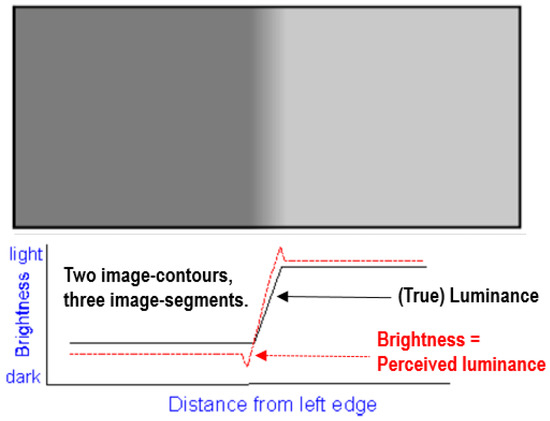 Figure 9. Mach bands illusion [13,156]. In black: Ramp in luminance units across space. In red: Brightness (perceived luminance) across space. One of the best-known brightness illusions, where brightness is defined as a subjective aspect of vision, i.e., brightness is the perceived luminance of a surface, is the psychophysical phenomenon of the Mach bands: where a luminance (radiance, intensity) ramp meets a plateau, there are spikes of brightness, although there is no discontinuity in the luminance profile. Hence, human vision detects two boundaries, one at the beginning and one at the end of the ramp in luminance. Since there is no discontinuity in luminance where brightness is spiking, the Mach bands effect is called a visual “illusion”. Along a ramp, no image-contour is perceived by human vision, irrespective of the ramp’s local contrast (gradient) in range (0, +∞). In the words of Pessoa, “if we require that a brightness model should at least be able to predict Mach bands, the bright and dark bands which are seen at ramp edges, the number of published models is surprisingly small” [156]. In 2D signal (image) processing, the important lesson to be learned from the Mach bands illusion is that local variance, contrast and first-order derivative (gradient) are statistical features (data-derived numeric variables) computed locally in the (2D) image-domain not suitable to detect image-objects (segments, closed contours) required to be perceptually “uniform” (“homogeneous”) in agreement with human vision. In other words, these popular local statistics, namely, local variance, contrast and first-order derivative (gradient), are not suitable visual features if detected image-segments/image-contours are required to be consistent with human visual perception, including ramp-edge detection. This straightforward (obvious), but not trivial observation is at odd with a large portion of the existing computer vision (CV) and remote sensing (RS) literature, where many semi-automatic image segmentation/image-contour detection algorithms are based on thresholding the local variance, contrast or first-order gradient, e.g., [157,158,159], where a system’s free-parameter for thresholding image-objects or image-contours must be user-defined in range ∈ (0, +∞) based on heuristics.
Although it is largely ignored by large portions of the RS community, the unequivocal true fact that inherently ill-posed CV ⊃ EO-IU algorithms for radiometric Cal of DNs into SURF or surface albedo values do require EO image classification to be performed in advance is implicitly confirmed by existing open source or commercial software toolboxes for EO image enhancement (pre-processing), critically reviewed hereafter.
Supported by NASA, the baseline of the U.S. Landsat ARD format [139,140,141,142,143] is atmospheric effect removal by the open source Landsat-4/5/7 Ecosystem Disturbance Adaptive Processing System (LEDAPS). In LEDAPS, exclusion masks for water, cloud, shadow and snow surface types were detected by an over-simplistic set of prior knowledge-based spectral decision rules applied per pixel [146]. Quantitative analyses of LEDAPS products led by its authors revealed that these exclusion masks were prone to errors, to be corrected in future LEDAPS releases [146]. The same considerations hold for the Landsat 8 OLI/TIRS-specific Landsat Surface Reflectance Code (LaSRC) [160] adopted by the U.S. Landsat ARD format [139,140,141,142,143]. Unfortunately, suitable for testing or Val purposes, a multi-level image consisting of exclusion masks has never been generated as standard output by either LEDAPS or LaSRC. To detect quality layers cloud and cloud–shadow, in addition to snow/ice pixels, recent versions of LEDAPS and LaSRC adopted the open source C Function of Mask (CFMask) algorithm [139,140]. CFMask was derived from the open source Function of Mask (FMask) algorithm [58,59], translated into the C programming language to facilitate its implementation in a production environment. Unfortunately, to date, in a recent comparison of cloud and cloud–shadow detectors, those implemented in LEDAPS scored low among alternative solutions [62]. By the way, potential users of U.S. Landsat ARD imagery are informed by USGS in advance about typical CFMask artifacts [63]. Like other cloud detection algorithms [61,62], CFMask may have difficulties over bright surface types such as building tops, beaches, snow/ice, sand dunes, and salt lakes. Optically thin clouds will always be challenging to identify and have a higher probability of being omitted by the U.S. Landsat ARD algorithm. In addition, the algorithm performance has only been validated for cloud detection, and to a lesser extent for cloud shadows. No rigorous evaluation of the snow/ice detection has ever been performed [63].
Transcoded into CFMask by the U.S. Landsat ARD processor, the open source Fmask algorithm for cloud, cloud–shadow and snow/ice detection was originally developed for single-date 30 m resolution 7-band (from visible blue, B, to thermal InfraRed, TIR) Landsat-5/7/8 MS imagery, which includes a thermal band as key input data requirement [58]. In recent years, FMask was extended to 10 m/20 m resolution Sentinel-2 MS imagery [59], featuring no thermal band, and to Landsat image time-series (multiTemporal Mask, TMask) [60]. For more details about the FMask software design and implementation, refer to the further Section 3.
In the Atmospheric/Topographic Correction for Satellite Imagery (ATCOR) commercial software product, several per-pixel (spatial context-insensitive) deductive spectral rule-based decision trees are implemented for use in different stages of an EO image enhancement pipeline [71,72,73,74,161,162], see Figure 10. According to Richter and Schläpfer [71,72], “pre-classification as part of the atmospheric correction has a long history, e.g., in the NASA’s processing chain for MODIS” [57], also refer to [12,56]. One of the ATCOR’s prior knowledge-based per-pixel decision trees delivers as output a haze/cloud/water (and snow) classification mask file (“image_hcw.bsq”), see Table 3. In addition, ATCOR includes a so-called prior knowledge-based decision tree for Spectral Classification of surface reflectance signatures (SPECL) [73], see Table 4. Unfortunately, SPECL has never been tested by its authors in the RS literature, although it has been validated by independent means [161,162].
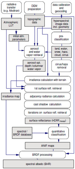
Figure 10.
As in [74], courtesy of Daniel Schläpfer, ReSe Applications Schläpfer. A complete (“augmented”) hybrid (combined deductive and inductive) inference workflow for multi-spectral (MS) image correction from atmospheric, adjacency and topographic effects. It combines a standard Atmospheric/Topographic Correction for Satellite Imagery (ATCOR) commercial software workflow [71,72], with a bidirectional reflectance distribution function (BRDF) effect correction, which requires as input an image time-series of the same surface area acquired with different combinations of the sun and sensor positions. Processing blocks are represented as circles and output products as rectangles. This hybrid workflow alternates deductive/prior knowledge-based and inductive/learning-from-data inference units, starting from initial conditions provided by a first-stage prior knowledge-based decision tree for static (non-adaptive to data) color naming, such as the Spectral Classification of surface reflectance signatures (SPECL) decision tree [73] implemented within the ATCOR commercial software toolbox. Categorical variables generated as output by the two processing blocks identified as “pre-classification” and “classification” are employed as input by the subsequent processing blocks to stratify (mask) unconditional numeric variable distributions, in line with the statistic stratification principle [152]. Through statistic stratification, inherently ill-posed inductive learning-from-data algorithms are provided with a priori knowledge required in addition to data to become better posed for numerical solution, in agreement with the machine learning-from-data literature [32,33].
Table 3.
Thematic map legend of the ATCOR-2/3/4 spectral pre-classification [71,72,73], whose output product is identified as “image_hcw.bsq” (hcw = haze/cloud/water and snow) map. According to Richter and Schläpfer, “pre-classification as part of the atmospheric correction has a long history, e.g., as part of NASA’s processing chain for MODIS”, e.g., refer to [57].
Table 4.
Rule set (structural knowledge) and order of presentation of the rule set (procedural knowledge) adopted by the prior knowledge-based MS reflectance space quantizer, eligible for MS reflectance space hyperpolyhedralization into MS color names, called Spectral Classification of surface reflectance signatures (SPECL), implemented within the ATCOR commercial software toolbox [71,72,73].
Commissioned by ESA, the Sentinel-2 (atmospheric and topographic) Correction Prototype Processor (Sen2Cor) is not run systematically at the ESA ground segment. Rather, it can be downloaded free-of-cost from an ESA website to be run on the user side [11,12,44]. Hence, the ESA Sen2Cor software toolbox does not satisfy the ESA EO Level 2 product requirements specification, refer to Section 1. The existing sensor-specific Sen2Cor prototype processor, sketched in Figure 11, adopts the same feedforward workflow of the popular ATCOR commercial software product [71,72,73]. The Sen2Cor software toolbox accomplishes, first, one SCM product generation from TOARF values by means of a per-pixel (spatial context-insensitive) prior spectral knowledge-based (static, non-adaptive to data) decision tree, whose SCM legend is shown in Table 1. Next, a stratified (class-conditional, driven-by-knowledge) MS image radiometric correction approach is adopted to transform TOARF into SURF values, where SURF values are sequentially corrected for atmospheric, adjacency and topographic effects stratified by the same SCM product generated at first stage from TOARF values.
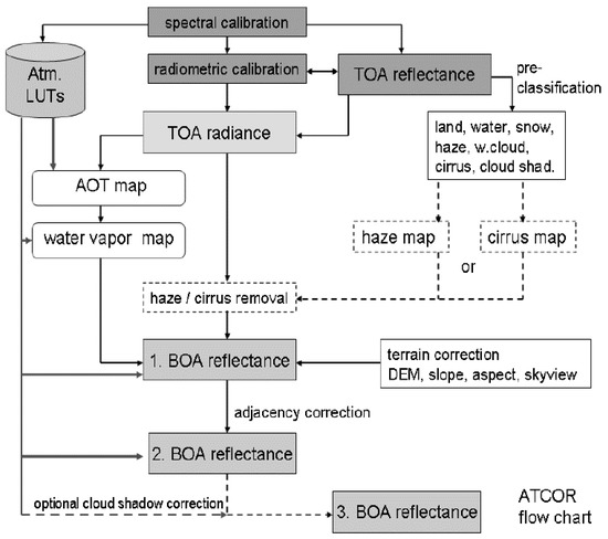
Figure 11.
Sen2Cor flow chart for ESA Level 2 product generation from Sentinel-2 imagery [11,12,44], same as in the Atmospheric/Topographic Correction for Satellite Imagery (ATCOR) commercial software toolbox [71,72,73]. While sharing the same system design, ESA Sen2Cor and ATCOR differ at the two lowest levels of abstraction, known as algorithm and implementation [76] (refer to Section 1). First, a scene classification map (SCM) is generated from top-of-atmosphere reflectance (TOARF) values. Next, class-conditional MS image radiometric enhancement of TOARF into surface reflectance (SURF) values, synonym for bottom-of-atmosphere (BOA) reflectance values, corrected for atmospheric, adjacency and topographic effects is accomplished in sequence, stratified by the same SCM product generated at first stage from TOARF values. More acronyms in this figure: AOT = aerosol optical thickness, DEM = digital elevation model, LUT = look-up table.
To overcome structural limitations in system design of existing open source or commercial software products for EO image radiometric Cal (correction, in general), such as Sen2Cor, ATCOR, LEDAPS and LaSRC, a viable alternative is an inherently ill-posed atmospheric, topographic, adjacency and BRDF effect correction system architecture sketched as in Figure 12 [13,82,83], to be considered as the third original contribution of this review section. The estimation from an input numeric variable, starting from EO sensory data equivalent to DNs provided with no physical meaning, of an output numeric variable provided with a physical meaning of increasing quality, such as EO data-derived TOARF, SURF and spectral albedo values featuring increasing levels of radiometric Cal quality, requires as additional input, at each stage of the EO image enhancement flow chart, a categorical (nominal) variable belonging to a preliminary SCM automatically generated from the EO image radiometrically corrected at the previous stage in the workflow. In other words, equivalent to two sides of the same coin, categorical variables (e.g., SCMs at increasing levels of mapping accuracy and semantics) and continuous variables (e.g., TOARF, SURF and spectral albedo values) should be estimated from raw EO imagery (coded as dimensionless DNs, provided with no physical meaning) alternately and hierarchically [13,107,147,148,149]. It means that, in an EO image pre-processing workflow conceived of as a hierarchical hybrid inference system, such as the stratified topographic correction (STRATCOR) algorithm proposed in [13,107], categorical variables of hierarchically increasing quality in semantics and accuracy are estimated from (hierarchically enhanced) continuous variables, where a priori knowledge is required in addition to data to make an inherently ill-posed data classification problem better posed for numerical solution [13,33,82,83,118]. This hierarchical classification approach alternates with a numeric variable estimation stage of hierarchically increasing radiometric quality, which is conducted on a categorical (stratified, masked, class-conditional) basis, where data stratification is required to make the inherently ill-posed radiometric correction stage, either atmospheric, topographic, adjacency or BRDF effect correction, better posed for numeric solution [13,33,82,83,107,118], see Figure 12.
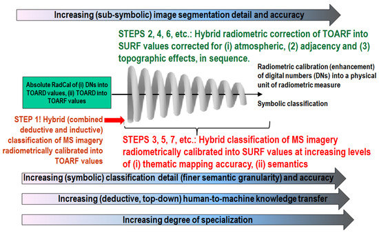
Figure 12.
Ideal ESA EO Level 2 product generation design as a hierarchical alternating sequence of: (A) hybrid (combined deductive and inductive) radiometric enhancement of multi-spectral (MS) dimensionless digital numbers (DNs) into top-of-atmosphere reflectance (TOARF), surface reflectance (SURF) values and spectral albedo values corrected in sequence for (1) atmospheric, (2) adjacency, (3) topographic and (4) BRDF effects, and (B) hybrid (combined deductive and inductive) classification of TOARF, SURF and spectral albedo values into a sequence of ESA EO Level 2 scene classification maps (SCMs), whose legend (taxonomy) of community-agreed land cover (LC) class names, in addition to quality layers cloud and cloud–shadow, increases hierarchically in semantics and mapping accuracy. An implementation in operating mode of this EO image pre-processing system design for stratified topographic correction (STRATCOR) is presented and discussed in [13,82,83,107]. In comparison with this desirable system design, let us consider that, for example, the existing Sen2Cor software toolbox, developed by ESA to support a Sentinel-2 sensor-specific Level 2 product generation on the user side [11,12,44], adopts no hierarchical alternating approach between MS image classification and MS image radiometric enhancement. Rather, ESA Sen2Cor accomplishes, first, one SCM generation from TOARF values based on a per-pixel (spatial context-insensitive) prior spectral knowledge-based decision tree. Next, a class-conditional MS image radiometric enhancement of TOARF into SURF values corrected for atmospheric, adjacency and topographic effects is accomplished in sequence, stratified by the same SCM product generated at first stage from TOARF values, see Figure 11.
As the fourth original contribution of this review section, it is worth recalling here that TOARF, SURF and surface albedo values, estimated as intermediate or final data products by an ESA EO Level 2 product generator and whose physical domain of change is 0.0–1.0, can be rescaled to the discrete and finite range {0, 255} according to an unsigned char data coding expression, e.g., byte(SURF/255. + 0.5) where operator byte() truncates any decimal part of a number whose data type is float. If byte coded into range {0, 255}, then TOARF, SURF and surface albedo values, whose physical range is 0.0–1.0, are affected by a quantization (discretization) error equal to (Max − Min)/number of bins/2 (due to rounding to the closest integer, either above or below) = (1.0 − 0.)/255/2. = 0.002 = 0.2%, to be considered negligible. It means that, in addition to providing DNs with a physical unit of radiometric measure, where DNs in EO Level 0 up to Level 2 imagery are typically coded as 16-bit unsigned short integer [139,140,141,142,143,163], radiometric Cal of DNs into TOARF, SURF and surface albedo values at either EO Level 1 or Level 2 imagery allows pixel coding as 8-bit unsigned char, with a 50% save in memory storage at the cost of a 0.2% quantization error. This observation, though straightforward, is neither obvious nor trivial. In practice, for example, the Planet Surface Reflectance (SR) Product [163] and the U.S. Landsat ARD format [139,140,141,142,143], coded as a 16-bit unsigned short integer, can be transcoded into an 8-bit unsigned char, affected by a quantization error as low as 0.2%, with a 50% save in memory storage. For comparison purposes, it is worth recalling here that when per-image metadata files of radiometric parameters (e.g., gain, offset, acquisition time, etc.) are available to transform, first, DNs into top-of-atmosphere radiance (TOARD) values, based on a band-specific gain and offset metadata parameter pair, with TOARD values ≥ 0, and, next, to transform TOARD values into TOARF values belonging to range 0.0–1.0, it is well known that a typical approximation of the sun-Earth distance to 1 independent of the image-specific acquisition time typically causes TOARF estimation errors of about 3–5% [67,143]. Despite common practice, where the sun-Earth distance estimation is oversighted by large portions of the RS community, in [143] a community-agreed standardization of the sun-Earth distance estimation in radiometric Cal methodologies was recommended for improved harmonization/interoperability of multi-sensor multi-temporal EO big data cubes.
3. Related Works in Cloud and Cloud–Shadow Quality Layers Detection
Cloud and cloud–shadow quality layers detection (see Figure 13 and Figure 14) in operating mode (refer to Section 2) is considered an open problem to date by the RS community [61,62,63]. Provided with a relevant survey value, this Section critically reviews standard cloud/cloud–shadow detectors, available either open source or free-of-cost, at the Marr five levels of abstraction of an information processing system (refer to Section 1) [13,19,76,82,83].
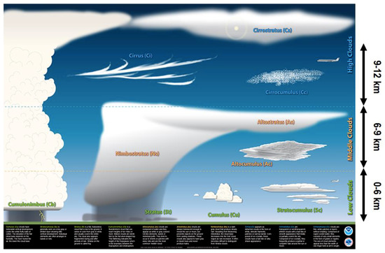
Figure 13.
Cloud classification according to the U.S. National Weather Service adapted from [164].
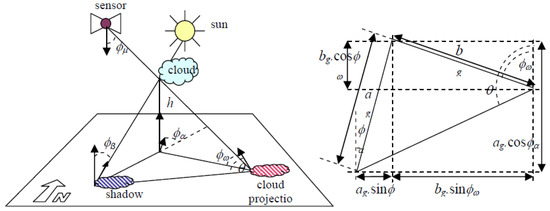
Figure 14.
Adapted from [55]. Sun-cloud-satellite geometry for arbitrary viewing and illumination conditions. Left: Actual 3D representation of the Sun/cloud/cloud–shadow geometry. Cloud height, h, is a typical unknown variable. Right: Apparent Sun/cloud/cloud–shadow geometry in a 2D soil projection, with ag = h ⋅ tanφβ, bg = h ⋅ tanφμ.
In the last decade, many different cloud/cloud–shadow detection algorithms have been presented in the RS literature [12,13,43,44,45,46,47,48,49,50,51,52,53,54,55,56,57,58,59,60], to be input with either a single-date MS image or an MS image time-series typically acquired by either one EO spaceborne/airborne MS imaging sensor or a single family of MS imaging sensors, e.g., the Landsat family of spaceborne MS imaging sensors.
Predated by a long history of deductive (physical model-based) convolutional neural networks (CNNs), consisting of “handcrafted” multi-scale 2D spatial filter banks developed since the early 1980s for multi-scale image analysis (encoding, decomposition) [13,76,87,88,89,90,91,92,93,94,95,96,97,98,99,100,101,102,103,104], synthesis (decoding, reconstruction) [94] and classification (understanding) [76,95], the recent hype about end-to-end inductive learning-from-data DCNNs in CV applications [34,35,36,37,38] is progressively affecting the RS discipline, in spite of increasing disillusionment in the AI community [13,30,64,88,165,166,167,168,169]. For example, an increasing number of DCNN applications for cloud detection can be found in the RS literature, such as [42]. However, to our best knowledge, only one application of DCNNs to the simultaneous (joint) detection of cloud and cloud–shadow phenomena exists to date, where cloud-shadow detection is affected by very low mapping quality indicators [35].
To explain this fact, a non-trivial understanding of the information/knowledge representation in DCNNs is required, according to the Marr five levels of understanding of an information processing system (refer to Section 1) [13,19,76,82,83]. In inductive learning-from-data DCNNs [34,35,36,37,38], 2D spatial filter profiles are learned end-to-end from supervised image examples whereas a priori knowledge is encoded by design based on heuristics, a.k.a. trial-and-error. In more detail (refer to Section 2), the whole set of DCNN architectural metaparameters, specifically, number of layers, number of convolutional filters per layer, filter size, inter-filter stride, subsampling filter size, subsampling inter-filter stride, etc., is user-defined based on empirical criteria. Unfortunately, inductive learning-from-data algorithms, including DCNNs, are affected by inherent limitations [2,13,30,33,40,41,64,88,165,166,167] and known failure modes [168,169], including the following. Suitable for learning complex correlations between input and output features, inductive learning-from-data systems are unable to learn representations of causality (cause–effect relationships, dependency), known that “correlation does not imply causation and vice versa” [13,19,30,33,64,65]. This limitation implies that, first, integration of a priori knowledge about the physical real-world onto a DCNN architecture is typically not a straightforward task because, in DCNNs, information representation pertains mainly to (largely opaque, unknown a priori) correlations between input and output features. Second, DCNNs thus far have shown no self-organizing capability, e.g., based on combinations of cooperative with competitive learning-from-data policies [170], suitable for developing a syntactic hierarchical system [19,30], structured as a network of specialized subnetworks [13], in agreement with the engineering principles of modularity, hierarchy and regularity considered necessary for scalability in structured system design [39]. In the words of Marcus, “the core problem, at least at present, is that deep learning learns correlations between sets of features that are themselves “flat” or non-hierarchical, as if in a simple, unstructured list, with every feature on equal footing. Hierarchical structures (e.g., syntactic trees that distinguish between main clauses and embedded clauses in a sentence) are not inherently or directly represented in such systems, and as a result deep learning systems are forced to use a variety of proxies that are ultimately inadequate, such as the sequential position of a word presented in a sequences” [30].
Our straightforward, but not trivial conjecture (refer to Section 1) was that joint cloud and cloud–shadow detection is a typical example of physical model-based cause–effect relationship expected to be very difficult to solve by inductive machine learning-from-examples algorithms, including DCNNs [34] designed for semantic segmentation [37] and instance segmentation [38] (excluding DCNNs for object detection by rounding box localization, such as [36], inapplicable per se to the cloud/cloud-detection problem of interest, pertaining to the domain of so-called semantic segmentation problems), which are typically suitable for learning complex correlations between input and output features, but unable to discover inherent representations of causality.
This conjecture is perfectly confirmed by experimental conclusions reported in [35] (pp. 32,33) where the quote is: “The main problem of DCNN-based classification is cloud–shadow, e.g., in an image object-based Intersection over Union, IoU, for image object-based classification quality measure assessment in range 0.0–1.0, class cloud–shadow scored as low as IoU = 0.0212 in the validation image set at hand”. Predicted by theory, these experimental results prove a posteriori the well-grounded nature of our first-principles in the AI ⊃ CV domains. These expected results reveal that, based on knowledge of inference first-principles, specifically, induction, deduction and abduction [19,22,24], and in agreement with the increasing disillusionment of the AI community about deep learning-from-data [13,30,64,88,165,166,167,168,169], the RS community should avoid exploring dead-end solutions where AI ⊃ CV algorithms, originally developed by other communities in the cognitive science domain (see Figure 2), such as increasingly popular DCNNs [34,35,36,37,38], are adopted as black-boxes by RS scientists and practitioners for detecting cloud and cloud–shadow cause–effect-relationships in multi-sensor EO imagery at large-scale. Based on this rationale, although considered state-of-the-art by the mainstream CV and RS audience, DCNN solutions [34,35,36,37,38] are excluded from any further review in this paper, focused on the joint detection of cloud and cloud–shadow quality layers featuring an inter-layer cause–effect relationship.
For comparison purposes, three popular computer programs available either open source or free-of-cost for cloud/cloud–shadow detection in spaceborne MS imagery are critically reviewed hereafter, see Table 5.
Table 5.
Comparison of alternative joint cloud and cloud–shadow detection algorithms at three levels of understanding of an information processing system proposed by Marr, specifically, information/knowledge representation, system design (architecture) and algorithm (refer to Section 1) [13,19,76,82,83].
- The single-date multi-sensor FMask open source algorithm [58], originally developed for single-date 30 m resolution 7-band (from visible blue, B, to thermal InfraRed, TIR) Landsat-5/7/8 MS imagery, which includes a thermal band as key input data requirement. FMask was recently extended to 10 m/20 m resolution Sentinel-2 MS imagery [59], featuring no thermal band, and to Landsat image time-series (multiTemporal Mask, TMask) [60]. The potential relevance of FMask is augmented by considering that CFmask, an Fmask program version transcoded into the C programming language for increased efficiency, is adopted for cloud, cloud–shadow and snow/ice classification by the LEDAPS and LaSRC algorithms for atmospheric correction in the U.S. Landsat ARD product [139,140,141,142,143]. Unfortunately, CFMask is affected by known artifacts [63]. Moreover, in a recent comparison of cloud and cloud–shadow detectors, those implemented in LEDAPS scored low among alternative solutions [62].
- The single-date single-sensor ESA Sen2Cor prototype processor, capable of automated atmospheric, adjacency and topographic effect correction and SCM product generation, including cloud and cloud–shadow detection (refer to the SCM legend shown in Table 1), whose input is an ESA EO Level 1 image, radiometrically calibrated into TOARF values, originally acquired at Level 0 (in dimensionless DNs provided with no radiometric unit of measure) by the ESA Sentinel-2 Multi-Spectral Instrument (MSI) exclusively. The ESA Sen2Cor prototype processor is distributed free-of-cost by ESA to be run on the user side [11,12]. Hence, it does not satisfy the ESA EO Level 2 product requirements specification proposed in Section 1. ESA Sen2Cor incorporates capabilities of the ATCOR commercial software toolbox [71,72,73], see Figure 11. ESA Sen2Cor is affected by known artifacts [44,47,61], which may be inherited at least in part from ATCOR.
- The multi-date multi-sensor MAJA, developed and run by CNES/CESBIO/DLR [46,48]. Starting from its name, MAJA incorporates capabilities of the ATCOR commercial software toolbox [71,72,73]. MAJA is affected by known artifacts [47,61], which may be inherited at least in part from ATCOR.
Table 5 compares the Sen2cor, MAJA and FMask computer programs at three-of-five levels of understanding of an information processing system proposed by Marr, specifically, information/knowledge representation, system design (architecture) and algorithm (refer to Section 1) [13,19,76,82,83]. For the sake of brevity, Table 5 omits comparisons of alternative algorithms at the two levels of understanding known as outcome/process requirements specification and implementation (refer to Section 1).
The first observation stemming from Table 5 is that Sen2cor and MAJA employ deductive (top-down, prior knowledge-based) inference, exclusively, to map MS imagery onto LC classes, in addition to mapping quality layers cloud and cloud–shadow. This is in contrast with biological cognitive systems [108], where hybrid inference combines deductive and inductive inference to take advantage of each and overcome their shortcomings [2,13,40,41,82,83], refer to Section 2.
The second observation driven from Table 5 is that the Sen2cor, MAJA and FMask computer programs employ 1D image analysis algorithms exclusively, either pixel-based, i.e., spatial context-insensitive and spatial topology non-preserving, or spatial context-sensitive (e.g., image object-based or local window-based), but spatial topology non-preserving (non-retinotopic) [13,87,88,96,170]. In CV programs, 1D image analysis is a methodological (structural) drawback because perceptual evidence proves that, in vision, primary spatial topological information (e.g., adjacency, inclusion, etc.) and spatial non-topological information (e.g., spatial distance, angle measure) components dominate secondary color information [23], which is the sole information available at the imaging sensor’s spatial resolution, i.e., at the pixel level of spatial analysis, refer to Section 2 [13]. Intuitively, 1D image analysis algorithms are invariant to permutations in the 1D vector data sequence generated from a (2D) image, where image is synonym for 2D gridded data set, see Figure 15 [34]. In short, 1D analysis of (2D) imagery is affected by a loss in data dimensionality.
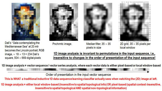
Figure 15.
Example of 1D image analysis, which is spatial topology non-preserving (non-retinotopic) in a (2D) image-domain [13,87,88,96,170]. Intuitively, 1D image analysis is insensitive to permutations in the input data set [34]. Synonym for 1D analysis of a 2D gridded data set, 1D image analysis is affected by spatial data dimensionality reduction. The (2D) image at left is transformed into the 1D vector data stream (sequence) shown at bottom, where vector data are either pixel-based or spatial context-sensitive, e.g., local window-based. This 1D vector data stream means nothing to a human photo interpreter. When it is input to either an inductive learning-from-data classifier or a deductive learning-by-rule classifier, the 1D vector data sequence is what the classifier actually sees when watching the (2D) image at left. Undoubtedly, computers are more successful than humans in 1D image analysis. Nonetheless, humans are still far more successful than computers in 2D image analysis, which is spatial context-sensitive and spatial topology-preserving (retinotopic) (see Figure 16).
Viable alternative to 1D image analysis is 2D image analysis, which is spatial context-sensitive and spatial topology-preserving (retinotopic) [13,87,88,96,170], i.e., it is sensitive to permutations in the order of presentation of the input 2D data set [34], see Figure 16. In our understanding, 2D spatial topology-preserving mapping is the fundamental basis of success of multi-scale 2D spatial filter banks for image analysis (encoding, decomposition), synthesis (decoding, reconstruction) and classification (understanding), either deductive/physical model-based [13,76,87,88,89,90,91,92,93,94,95,96,97,98,99,100,101,102,103,104] or end-to-end inductive learning-from-data, such as DCNNs [34,35,36,37,38].
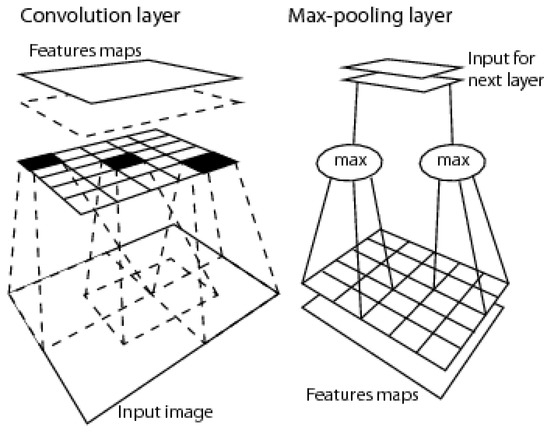
Figure 16.
2D image analysis is synonym for spatial context-sensitive and spatial topology-preserving (retinotopic) feature mapping in a (2D) image-domain [13,87,88,96,170]. Intuitively, 2D image analysis is sensitive to permutations in the input data set [34]. Activation domains of physically adjacent processing units in the 2D array of convolutional spatial filters are spatially adjacent regions in the 2D visual field. Provided with a superior degree of biological plausibility in modelling 2D spatial topological and spatial non-topological information components, distributed processing systems capable of 2D image analysis, such as deep convolutional neural networks (DCNNs), typically outperform traditional 1D image analysis approaches. Will computers ever become as good as humans in 2D image analysis?
The fundamental difference between 1D image analysis and 2D image analysis with regard to spatial topology-preserving (retinotopic) feature mapping [13,87,88,96,170] is at the basis of a proposed revision of the loose GE(OBIA) paradigm [10] into a more restrictive definition of EO imagery for Geographical Sciences (EO4GEO), synonym for 2D analysis of EO (2D) imagery for GISCience applications [129,130], see Figure 17.
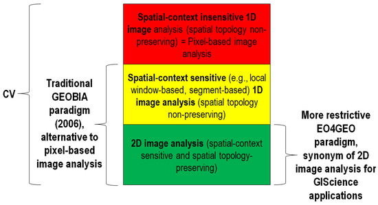
Figure 17.
EO for Geographical Sciences (EO4GEO, EO4GIScience) framework, meaning EO big data analytics in operating mode for GIScience applications, constrained by 2D (retinotopic, spatial topology-preserving) image analysis in cognitive science [129]. EO4GEO is more restrictive than the traditional GEOBIA paradigm, formalized in 2006 and 2014 as a viable alternative to 1D spatial context-insensitive (pixel-based) image analysis [9,10,130].
At the Marr two lowest levels of understanding of an information processing system, i.e., algorithm and implementation (refer to Section 1) [13,19,76,82,83], it is interesting to investigate the ESA Sen2Cor’s static (non-adaptive to data, prior knowledge-based) per-pixel spectral rule-based decision tree implementation for automated ESA EO Level 2 SCM product generation [12]. The same considerations driven from the Sen2Cor’s spectral knowledge-based decision tree implementation for SCM generation hold for the LEDAPS, LaSRC and ATCOR spectral knowledge-based decision trees, implemented for pixel-based pre-classification as necessary-but-not-sufficient pre-condition to make inherently ill-posed atmospheric and/or topographic correction algorithms better posed for numerical solution [32,33], see Section 2. According to Richter and Schläpfer [71,72], “pre-classification as part of the atmospheric correction has a long history, e.g., in the NASA’s processing chain for MODIS” [57].
First, in the interdisciplinary domain of cognitive science [18,77,78,79,80,81], it was highlighted that static (non-adaptive to data, prior knowledge-based) spectral rule-based decision trees aim at a mutually exclusive and totally exhaustive (hyper)polyhedralization of a MS reflectance (hyper)space, equivalent to (numeric) color space discretization into color names belonging to a categorical variable, known as color vocabulary [13,14,15]. Within the domain of cognitive science (see Figure 2), color naming was deeply investigated by linguistics. Central to this consideration is Berlin and Kay’s landmark study of a “universal” inventory of eleven basic color (BC) words in twenty human languages: black, white, gray, red, orange, yellow, green, blue, purple, pink and brown [171]. Suitable for color naming of MS imagery, MS reflectance (hyper)space (hyper)polyhedralization is difficult to think of and impossible to visualize when the MS data space dimensionality is superior to three, see Figure 18. This is not the case of basic color (BC) names adopted in human languages [171], whose mutually exclusive and totally exhaustive perceptual polyhedra, neither necessarily convex nor connected, are intuitive to think of and easy to visualize in a 3D monitor-typical red-green-blue (RGB) data cube [172], see Figure 19.
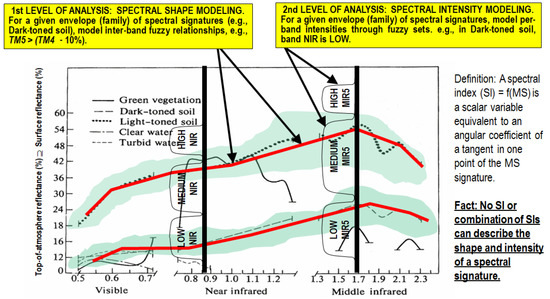
Figure 18.
Examples of land cover (LC) class-specific families of spectral signatures [17] in top-of-atmosphere reflectance (TOARF) values, which include surface reflectance (SURF) values as a special case in clear sky and flat terrain conditions [173], i.e., in general, TOARF ⊇ SURF, where TOARF ≈ SURF (depicted as an ideal “noiseless” spectral signature in red) + atmospheric and topographic noise. A within-class family of spectral signatures (e.g., dark-toned soil) in TOARF or SURF values forms a buffer zone (hyperpolyhedron, envelope, manifold, joint distribution), depicted in light green. Like a vector quantity has two characteristics, a magnitude and a direction, any LC class-specific MS manifold is characterized by a multivariate shape and a multivariate intensity information component. In the RS literature, typical prior knowledge-based spectral decision trees for MS reflectance space hyperpolyhedralization into a finite and discrete vocabulary of MS color names, such as Sen2Cor’s [12], MAJA’s [46,48], ATCOR’s [71,72], LEDAPS’ [139,140,146] and LaSRC’s [139,140,160], typically adopt either a multivariate analysis of spectral indexes or a logical (AND, OR) combination of univariate variables, such as scalar spectral indexes or spectral channels, considered mutually independent. A typical spectral index is a scalar band ratio or band-pair difference equivalent to an angular coefficient of a tangent to the spectral signature in one point. It is well known that infinite functions can feature the same tangent value in one point. In practice, no spectral index or combination of spectral indexes can reconstruct the multivariate shape and multivariate intensity information components of a spectral signature. As a viable alternative to traditional static (non-adaptive to data) spectral rule-based decision trees found in the RS literature, the Satellite Image Automatic Mapper (SIAM)’s prior knowledge-based spectral decision tree [13,14,15,82,83,107,118,132,133,161,162,174] adopts a convergence-of-evidence approach to model any target family (ensemble) of spectral signatures, forming a hypervolume of interest in the MS reflectance hyperspace, as a combination of multivariate shape information with multivariate intensity information components. For example, as shown above, typical spectral signatures of dark-toned soils and typical spectral signatures of light-toned soils form two MS envelopes in the MS reflectance hyperspace that approximately share the same multivariate shape information component, but whose pair of multivariate intensity information components does differ.
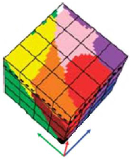
Figure 19.
Adapted from [172]. Unlike a MS reflectance space hyperpolyhedralization difficult to think of and impossible to visualize when the number of channels is superior to three, an RGB data cube polyhedralization is intuitive to think of and straightforward to display. For example, based on psychophysical evidence, human basic color (BC) names can be mapped onto a monitor-typical RGB data cube. Central to this consideration is Berlin and Kay’s landmark study of a “universal” inventory of eleven BC words in twenty human languages: black, white, gray, red, orange, yellow, green, blue, purple, pink and brown [171].
In vision, where a (2D) image-domain and a 4D geospatial-temporal scene-domain co-exist, see Figure 6, a community-agreed discrete and finite vocabulary of MS color names, pertaining to a MS color space in the image-domain, such as the eleven BC names proposed by Berlin and Kay in the image-domain of visible bands RGB [171], see Figure 19, should never be confused with a vocabulary of classes of real-world objects in the scene-domain, such as a discrete and finite legend of LC classes. Color names provide a categorical (nominal) representation of the numeric photometric variable associated as attribute to any LC class belonging to a discrete and finite LC class legend. Encoded as a categorical variable, a color attribute of a (categorical) LC class should never be confused with the LC class it belongs to. On the hand, the same color name can be shared by several LC classes. On the other hand, a single LC class can feature several color names as photometric attribute [14,15]. For example, Adams et al. correctly observed that discrete spectral endmembers typically adopted in hyper-spectral image interpretation “cannot always be inverted to unique LC class names” [175]. This commonsense knowledge is sketched in Table 6, where set A = DictionaryOfColorNames with cardinality |A| = a = ColorVocabularyCardinality = 11 and set B = LegendOfObjectClassNames with cardinality |B| = b = ObjectClassLegendCardinality = 3. Between the vocabulary A of color names in the image-domain and the vocabulary B of LC classes in the scene-domain there is a binary relationship, R: A ⇒ B, subset of the 2-fold Cartesian product A × B, i.e., R: A ⇒ B ⊆ A × B, where A ≠ B in general. The Cartesian product A × B is a set whose elements are ordered pairs of each instance of set A combined with each instance of set B. Hence, the size of the Cartesian product A × B is rows × columns = a × b, where a ≠ b in general. Noteworthy, Cartesian product A × B ≠ FrequencyCount(A × B), where FrequencyCount(A × B) is known as two-way contingency table, association matrix, cross tabulation, bivariate table, bivariate frequency table (BIVRFTAB) or confusion matrix [13,176,177,178,179,180].
Table 6.
Example of a binary relationship R: A ⇒ B ⊆ A × B from set A = DictionaryOfColorNames, with cardinality |A| = a = ColorVocabularyCardinality = 11, and the set B = LegendOfObjectClassNames, with cardinality |B| = b = ObjectClassLegendCardinality = 3, where A × B is the 2-fold Cartesian product between sets A and B. The Cartesian product of two sets A × B is a set whose elements are ordered pairs. The size of A × B is rows × columns = a × b. The dictionary LegendOfObjectClassNames is a superset of the typical taxonomy of land cover (LC) classes adopted by the RS community. “Correct” entry-pairs (marked with √) must be: (i) selected by domain experts based on a hybrid combination of deductive prior beliefs with inductive evidence from data and (ii) community-agreed upon, to be used by members of the community [14,15].
In spite of this commonsense knowledge, see Table 6, and in contrast with the unquestionable true fact that, in vision, primary spatial information dominates secondary color information in both the image-domain and the scene-domain [13,14,15,23], see Section 2, prior knowledge-based spectral decision trees for MS color space hyperpolyhedralization into color names implemented by the RS community typically assume that the vocabulary A of color names in the image-domain and the vocabulary B of LC classes in the scene-domain do coincide in cardinality, semantics and order of presentation. If hypothesis A = B holds true, then the binary relationship R: A ⇒ B ⊆ A × B ≠ FrequencyCount(A × B) becomes a bijective (injective and surjective) function, while the two-way confusion matrix FrequencyCount(A × B) becomes square, where the main diagonal guides the interpretation process [14,15]. This is the case of the LC map legend of an SCM product generated as output by a static decision tree of spectral rules implemented by the ATCOR software toolbox, see Table 3 and Table 4, and by the Sen2Cor software toolbox, see Table 1, where there is one spectral rule (or OR-combination of spectral rules) per LC class and vice versa. The unrealistic assumption that categorical variable A = DictionaryOfColorNames, with cardinality |A| = a = ColorVocabularyCardinality, coincides with categorical variable B = LegendOfObjectClassNames, with cardinality |B| = b = ObjectClassLegendCardinality, is undertaken at the abstract level of system understanding known as information/knowledge representation, which is typically considered one cornerstone of success of an information processing system [13,19,76,82,83]. This unrealistic assumption heavily affects all subsequent levels of abstraction, specifically, system design, algorithm and implementation (refer to Section 1), in agreement with the well-known information principle known as garbage in, garbage out (GIGO), synonym for error propagation through an information processing chain [14,15]. This error propagation effect affecting CV ⊃ EO-IU applications increases as the imaging sensor’s spatial resolution becomes finer, such as in EO high spatial resolution (HR, in range 1 m–30 m) and very high spatial resolution (VHR, < 1 m) image understanding tasks [17].
In addition to the unrealistic assumption that vocabularies of color names and vocabularies of LC class names coincide at the level of system understanding of information/knowledge representation, the implementation of the Sen2Cor’s spectral rules for MS reflectance space hyperpolyhedralization into MS color names appears inadequate to define mutually exclusive and totally exhaustive hyperpolyhedra, where each hyperpolyhedron is a multivariate data distribution (joint probability).
First, the ESA Sen2Cor algorithm models each joint probability by means of a single spectral rule as an and/or-combination of univariate distributions. It assumes a joint distribution is equivalent to a product of univariate distributions, which holds true if and only if univariate variables are mutually independent. This assumption is completely unrealistic when modeling manifolds of LC class-specific spectral signatures sampled at a discrete and finite set of spectral bands. These spectral band values are not statistically independent because they are LC class-dependent. In general, multivariate data statistics are more informative than a combination of univariate data statistics. For example, maximum likelihood data classification, accounting for multivariate data correlation and variance (covariance), is typically more accurate than parallelepiped data classification whose rectangular decision regions, equivalent to a concatenation of univariate data constraints, poorly fit multivariate data in the presence of bivariate cross-correlation [27]. As a typical example of this critical point, see Table 4, showing the SPECL decision tree instantiation proposed by the ATCOR software toolbox, where each spectral rule is implemented as a logical combination of univariate statistics.
Second, in the Sen2Cor’s spectral rule-based decision tree a spectral rule implementation typically adopts many spectral indexes in the definition of each hyperpolyhedron equivalent to a MS color name. Like a vector quantity has two characteristics, a magnitude and a direction, any LC class-specific MS manifold is characterized by a multivariate shape and a multivariate intensity information component, see Figure 18. A spectral index, implemented as either a band difference or a band ratio, is conceptually equivalent to the angular coefficient of a tangent to the spectral signature in one point. It is well known that infinite functions can pass through the same point with the same angular coefficient. It means that, although appealing due to its conceptual and numerical simplicity [2], any scalar spectral index, equivalent to a spectral slope, is a MS shape descriptor independent of the MS intensity. It is unable per se to represent either the multivariate shape information component or the multivariate intensity information component of a MS signature [13]. In other words, no spectral index or combination of spectral indexes provides a lossless reconstruction of the multivariate shape and multivariate intensity information components of a spectral signature [13,14,15]. Because of this spectral information loss, the number of scalar spectral indexes proposed in the RS literature is ever increasing [2], in the unrealistic attempt to extract a more informative scalar variable from a multivariate spectral signature. In some published works, the misuse of spectral indexes reaches its peak when, to simplify a multivariate spectral signature both conceptually and numerically, the number of univariate spectral indexes extracted from the spectral signature is superior to the number of spectral bands; in this no-win situation, no MS data compression is accomplished while a loss in spectral information is guaranteed. As a typical example of this second critical point, see Table 4, showing the SPECL decision tree instantiation proposed by the ATCOR software toolbox where several band ratios are employed for modeling a MS hyperpolyhedron of interest in the MS data hyperspace.
4. Conclusions
For the sake of readability this paper is divided in two. To highlight the importance of a “universal” AutoCloud+ CV software for systematic cloud and cloud–shadow quality layers detection in multi-sensor, multi-angular and multi-temporal EO big data cubes, the present Part 1 discloses AutoCloud+ in a broad context of systematic ESA EO Level 2 product generation at the ground segment [11,12] or space segment [84,85,144,163], whose necessary-but-not-sufficient pre-condition is cloud/cloud–shadow quality layers detection in operating mode (refer to Section 2). The subsequent Part 2 (see Supplementary Materials) copes with the AutoCloud+ CV software system requirements specification, information/knowledge representation, system design, algorithm, implementation and preliminary experimental results.
Original contributions and main conclusions of the present Part 1 are summarized hereafter.
Conceptual in nature and pertaining to the interdisciplinary domain of cognitive science [18,77,78,79,80,81], see Figure 2, our working hypothesis is the first original contribution of this RTD study, see Figure 4 and Equation (1). Working hypothesis (1) postulates that systematic ESA EO Level 2 product generation in operating mode [11,12], whose part-of is cloud and cloud–shadow quality layer detection, is necessary-but-not-sufficient pre-condition for multi-sensor multi-temporal and multi-angular EO big data cube analytics as part-of the GEO-CEOS visionary goal of a GEOSS [5], never accomplished to date by the RS community. The general notion of GEOSS encompasses open sub-problems, such as semantic content-based image retrieval (SCBIR) + semantics-enabled information/knowledge discovery (SEIKD) = artificial general intelligence (AI) for Data and Information Access Services (AI4DIAS) at the ground segment. Dependence relationship (1) means that the GEOSS open problem, together with its still-unsolved (open) sub-problems of SCBIR and SEIKD, cannot be accomplished until the necessary-but-not-sufficient pre-condition of CV ⊃ EO image understanding (EO-IU) in operating mode, specifically, systematic ESA EO Level 2 product generation featuring cloud/cloud–shadow quality layers detection, is fulfilled in advance.
The second original contribution of the present Part 1 is both conceptual and pragmatic in the definition of RS best practices, which is the focus of efforts made by intergovernmental organizations such as GEO and CEOS. In more detail, the ESA EO Level 2 product definition is regarded as baseline information primitive (unit of EO data-derived information) eligible for use as “augmented” (enhanced) EO Analysis Ready Data (ARD) format, to be adopted as horizontal policy for standardization purposes by a “seamless innovation chain” needed for a new era of Space 4.0 [66], see Figure 8. Such an “augmented” EO ARD definition is more restrictive (in terms of output product requirements specification), more informative (in terms of physical and conceptual/semantic quality of numeric and categorical output products, respectively), but more difficult to be inferred from EO sensory data than existing U.S. Landsat ARD [139,140,141,142,143] and CEOS ARD for Land (CARD4L) format definitions [138].
Supplementary Materials
The following are available online at http://www.mdpi.com/2220-9964/7/12/457/s1.
Author Contributions
Conceptualization, A.B. and D.T.; Methodology, A.B. and D.T.; Software, A.B. and D.T.; Validation, D.T.; Formal Analysis, A.B. and D.T.; Investigation, A.B. and D.T.; Resources, A.B. and D.T.; Data Curation, D.T.; Writing—Original Draft Preparation, A.B.; Writing—Review and Editing, A.B. and D.T.; Visualization, A.B. and D.T.; Supervision, D.T.; Project Administration, D.T.; Funding Acquisition, D.T.
Funding
This research was funded in part by the Austrian Science Fund (FWF) through the Doctoral College GIScience (DK W1237-N23) and by the Austrian Research Promotion Agency (FFG) with regard to project Sentinel-2 Semantic Data Cube (Sen2cube).
Acknowledgments
Andrea Baraldi thanks Prof. Raphael Capurro for his hospitality, patience, politeness and open-mindedness. The authors wish to thank the Editor-in-Chief, Associate Editor and reviewers for their competence, patience and willingness to help.
Conflicts of Interest
The authors declare no conflict of interest. The funders had no role in the design of the study; in the collection, analyses, or interpretation of data; in the writing of the manuscript, and in the decision to publish the results.
Abbreviations
- AI: Artificial general Intelligence
- AI4DIAS: Artificial Intelligence for Data and Information Access Services (at the ground segment)
- AI4Space: Artificial Intelligence for Space (segment)
- ARD: Analysis Ready Data (format)
- ATCOR: Atmospheric/Topographic Correction commercial sofwtare product
- AVHRR: Advanced Very High Resolution Radiometer
- BC: Basic Color
- BIVRFTAB: Bivariate Frequency Table
- Cal: Calibration
- Cal/Val: Calibration and Validation
- CBIR: Content-Based Image Retrieval
- CEOS: Committee on Earth Observation Satellites
- CESBIO: Centre d’Etudes Spatiales de la Biosphère
- CFMask: C (programming language version of) Function of Mask
- CLC: CORINE Land Cover (taxonomy)
- CNES: Centre national d’études spatiales
- CNN: Convolutional Neural Network
- CORINE: Coordination of Information on the Environment
- CV: Computer Vision
- DCNN: Deep Convolutional Neural Network
- DEM: Digital Elevation Model
- DIAS: Data and Information Access Services
- DLR: Deutsches Zentrum für Luft- und Raumfahrt (German Aerospace Center)
- DN: Digital Number
- DP: Dichotomous Phase (in the FAO LCCS taxonomy)
- DRIP: Data-Rich, Information-Poor (syndrome)
- EO: Earth Observation
- EO-IU: EO Image Understanding
- EO-IU4SQ: EO Image Understanding for Semantic Querying
- ESA: European Space Agency
- FAO: Food and Agriculture Organization
- FIEOS: Future Intelligent EO imaging Satellites
- FMask: Function of Mask
- GEO: Intergovernmental Group on Earth Observations
- GEOSS: Global EO System of Systems
- GIGO: Garbage In, Garbage Out principle of error propagation
- GIS: Geographic Information System
- GIScience: Geographic Information Science
- GUI: Graphic User Interface
- IGBP: International Global Biosphere Programme
- IoU: Intersection over Union
- IU: Image Understanding
- LAI: Leaf Area Index
- LC: Land Cover
- LCC: Land Cover Change
- LCCS: Land Cover Classification System (taxonomy)
- LCLU: Land Cover Land Use
- LEDAPS: Landsat Ecosystem Disturbance Adaptive Processing System
- MAACS: Multisensor Atmospheric Correction and Cloud Screening
- MAJA: Multisensor Atmospheric Correction and Cloud Screening (MACCS)-Atmospheric/Topographic Correction (ATCOR) Joint Algorithm
- mDMI: Minimally Dependent and Maximally Informative (set of quality indicators)
- MHP: Modular Hierarchical Phase (in the FAO LCCS taxonomy)
- MIR: Medium InfraRed
- MODIS: Moderate Resolution Imaging Spectroradiometer
- MS: Multi-Spectral
- MSI: (Sentinel-2) Multi-Spectral Instrument
- NASA: National Aeronautics and Space Administration
- NIR: Near InfraRed
- NLCD: National Land Cover Data
- NOAA: National Oceanic and Atmospheric Administration
- NP: Non-deterministic Polynomial
- OBIA: Object-Based Image Analysis
- OGC: Open Geospatial Consortium
- OP: Outcome (product) and Process
- OP-Q2I: Outcome and Process Quantitative Quality Index
- QA4EO: Quality Accuracy Framework for Earth Observation
- Q2I: Quantitative Quality Indicator
- RGB: monitor-typical Red-Green-Blue data cube
- RMSE: Root Mean Square Error
- RS: Remote Sensing
- RTD: Research and Technological Development
- SCBIR: Semantic Content-Based Image Retrieval
- SCM: Scene Classification Map
- SEIKD: Semantics-Enabled Information/Knowledge Discovery
- Sen2Cor: Sentinel 2 (atmospheric, topographic and adjacency) Correction Prototype Processor
- SIAM™: Satellite Image Automatic Mapper™
- STRATCOR: Stratified Topographic Correction
- SURF: Surface Reflectance
- TIR: Thermal InfraRed
- TM (superscript): (non-registered) Trademark
- TMask: Temporal Function of Mask
- TOA: Top-Of-Atmosphere
- TOARD: TOA Radiance
- TOARF: TOA Reflectance
- UAV: Unmanned Aerial Vehicle
- UML: Unified Modeling Language
- USGS: US Geological Survey
- Val: Validation
- VAPS: Value-Adding information Products and Services
- VQ: Vector Quantization
- WGCV: Working Group on Calibration and Validation
References
- Schaepman-Strub, G.; Schaepman, M.E.; Painter, T.H.; Dangel, S.; Martonchik, J.V. Reflectance quantities in optical remote sensing—Definitions and case studies. Remote Sens. Environ. 2006, 103, 27–42. [Google Scholar] [CrossRef]
- Liang, S. Quantitative Remote Sensing of Land Surfaces; John Wiley and Sons: Hoboken, NJ, USA, 2004. [Google Scholar]
- Group on Earth Observation/Committee on Earth Observation Satellites (GEO-CEOS). A Quality Assurance Framework for Earth Observation, Version 4.0. 2010. Available online: http://qa4eo.org/docs/QA4EO_Principles_v4.0.pdf (accessed on 17 November 2018).
- Yang, C.; Huang, Q.; Li, Z.; Liu, K.; Hu, F. Big Data and cloud computing: Innovation opportunities and challenges. Int. J. Digit. Earth 2017, 10, 13–53. [Google Scholar] [CrossRef]
- Group on Earth Observation (GEO). The Global Earth Observation System of Systems (GEOSS) 10-Year Implementation Plan. 2005. Available online: http://www.earthobservations.org/docs/10-Year%20Implementation%20Plan.pdf (accessed on 19 January 2012).
- Ghosh, D.; Kaabouch, N. A Survey on Remote Sensing Scene Classification Algorithms. WSEAS Trans. Signal Proc. 2014, 10, 504–519. [Google Scholar]
- Cheng, G.; Han, J. A survey on object detection in optical remote sensing images. ISPRS J. Photogramm. Remote Sens. 2016, 117, 11–28. [Google Scholar] [CrossRef]
- Lu, D.; Weng, Q. A survey of image classification methods and techniques for improving classification performance. Int. J. Remote Sens. 2007, 28, 823–870. [Google Scholar] [CrossRef]
- Blaschke, T.; Lang, S. Object based image analysis for automated information extraction-a synthesis. In Proceedings of the Measuring the Earth II ASPRS Fall Conference, San Antonio, CA, USA, 6–10 November 2006; pp. 6–10. [Google Scholar]
- Blaschke, T.; Hay, G.J.; Kelly, M.; Lang, S.; Hofmann, P.; Addink, E.; Feitosa, R.Q.; van der Meer, F.; van der Werff, H.; van Coillie, F.; et al. Geographic object-based image analysis–towards a new paradigm. ISPRS J. Photogram. Remote Sens. 2014, 87, 180–191. [Google Scholar] [CrossRef] [PubMed]
- European Space Agency (ESA). Sentinel-2 User Handbook, Standard Document; ESA: Paris, France, 2015. [Google Scholar]
- Deutsches Zentrum für Luft-und Raumfahrt e.V. (DLR); VEGA Technologies. Sentinel-2 MSI–Level 2A Products Algorithm Theoretical Basis Document; Document S2PAD-ATBD-0001; European Space Agency: Paris, France, 2011. [Google Scholar]
- Baraldi, A. Pre-Processing, Classification and Semantic Querying of Large-Scale Earth Observation Spaceborne/Airborne/Terrestrial Image Databases: Process and Product Innovations. Ph.D. Thesis, Agricultural and Food Sciences, Department of Agricultural Sciences, University of Naples “Federico II”, Naples, Italy, 2017. Available online: https://www.researchgate.net/publication/317333100_Pre-processing_classification_and_semantic_querying_of_large-scale_Earth_observation_spaceborneairborneterrestrial_image_databases_Process_and_product_innovations (accessed on 30 January 2018).
- Baraldi, A.; Humber, M.L.; Tiede, D.; Lang, S. GEO-CEOS stage 4 validation of the Satellite Image Automatic Mapper lightweight computer program for ESA Earth observation Level 2 product generation—Part 1: Theory. Cogent Geosci. 2018, 1467357. [Google Scholar] [CrossRef] [PubMed]
- Baraldi, A.; Humber, M.L.; Tiede, D.; Lang, S. GEO-CEOS stage 4 validation of the Satellite Image Automatic Mapper lightweight computer program for ESA Earth observation Level 2 product generation—Part 2: Validation. Cogent Geosci. 2018, 1467254. [Google Scholar] [CrossRef] [PubMed]
- Di Gregorio, A.; Jansen, L. Land Cover Classification System (LCCS): Classification Concepts and User Manual; FAO Corporate Document Repository; FAO: Rome, Italy, 2000; Available online: http://www.fao.org/DOCREP/003/X0596E/X0596e00.htm (accessed on 10 February 2012).
- Swain, P.H.; Davis, S.M. Remote Sensing: The Quantitative Approach; McGraw-Hill: New York, NY, USA, 1978. [Google Scholar]
- Capurro, R.; Hjørland, B. The concept of information. Annu. Rev. Inf. Sci. Technol. 2003, 37, 343–411. [Google Scholar] [CrossRef]
- Sonka, M.; Hlavac, V.; Boyle, R. Image Processing, Analysis and Machine Vision; Chapman & Hall: London, UK, 1994. [Google Scholar]
- Fonseca, F.; Egenhofer, M.; Agouris, P.; Camara, G. Using ontologies for integrated geographic information systems. Trans. GIS 2002, 6, 231–257. [Google Scholar] [CrossRef]
- Growe, S. Knowledge-based interpretation of multisensor and multitemporal remote sensing images. Int. Arch. Photogramm. Remote Sens. 1999, 32, 71. [Google Scholar]
- Laurini, R.; Thompson, D. Fundamentals of Spatial Information Systems; Academic Press: London, UK, 1992. [Google Scholar]
- Matsuyama, T.; Hwang, V.S. SIGMA–A Knowledge-Based Aerial Image Understanding System; Plenum Press: New York, NY, USA, 1990. [Google Scholar]
- Sowa, J. Knowledge Representation: Logical, Philosophical, and Computational Foundations; Brooks Cole Publishing Co.: Pacific Grove, CA, USA, 2000. [Google Scholar]
- Ahlqvist, O. Using uncertain conceptual spaces to translate between land cover categories. Int. J. Geogr. Inf. Sci. 2005, 19, 831–857. [Google Scholar] [CrossRef]
- Bossard, M.; Feranec, J.; Otahel, J. CORINE Land Cover Technical Guide–Addendum 2000; Technical Report No. 40; European Environment Agency: Copenhagen, Denmark, 2000. [Google Scholar]
- Lillesand, T.; Kiefer, R. Remote Sensing and Image Interpretation; John Wiley & Sons: New York, NY, USA, 1979. [Google Scholar]
- Belward, A. (Ed.) The IGBP-DIS Global 1 Km Land Cover Data Set “DISCover”: Proposal and Implementation Plans; IGBP-DIS Working Paper 13; International Geosphere Biosphere Programme, European Commission Joint Research Center, ISPRA: Varese, Italy, 1996. [Google Scholar]
- Dumitru, C.O.; Cui, S.; Schwarz, G.; Datcu, M. Information content of very-high-resolution SAR images: Semantics, geospatial context, and ontologies. IEEE J. Sel. Top. Appl. Earth Obs. Remote Sens. 2015, 8, 1635–1650. [Google Scholar] [CrossRef]
- Marcus, G. Deep Learning: A Critical Appraisal. arXiv, 2018; arXiv:1801.00631. Available online: https://arxiv.org/ftp/arxiv/papers/1801/1801.00631.pdf (accessed on 16 January 2018).
- Land Change Science; Gutman, G., Janetos, A.C., Justice, C.O., Moran, E.F., Mustard, J.F., Rindfuss, R.R., Skole, D., Turner, B.L., Cochrane, M.A., Eds.; Kluwer: Dordrecht, The Netherlands, 2004. [Google Scholar]
- Bishop, C.M. Neural Networks for Pattern Recognition; Clarendon: Oxford, UK, 1995. [Google Scholar]
- Cherkassky, V.; Mulier, F. Learning from Data: Concepts, Theory, and Methods; Wiley: New York, NY, USA, 1998. [Google Scholar]
- Cimpoi, M.; Maji, S.; Kokkinos, I.; Vedaldi, A. Deep filter banks for texture recognition, description, and segmentation. Int. J. Comput. Vis. 2014. [Google Scholar] [CrossRef] [PubMed]
- Bartoš, M. Cloud and Shadow Detection in Satellite Imagery. Master’s Thesis, Computer Vision and Image Processing, Faculty of Electrical Engineering, Department of Cybernetics, Czech Technical University, Prague, Czech Republic, 2017. [Google Scholar]
- Li, K.; Cheng, G.; Bu, S.; You, X. Rotation-Insensitive and Context-Augmented Object Detection in Remote Sensing Images. IEEE Trans. Geosci. Remote Sens. 2018, 56, 2337–2348. [Google Scholar] [CrossRef]
- Long, J.; Shelhamer, E.; Darrell, T. Fully convolutional networks for semantic segmentation. IEEE Trans. Pattern Anal. Mach. Intell. 2017, 39, 640–651. [Google Scholar]
- He, K.; Gkioxari, G.; Dol’ar, P.; Girshick, R. Mask R-CNN. arXiv, 2018; arXiv:1703.06870v3. [Google Scholar] [CrossRef] [PubMed]
- Lipson, H. Principles of modularity, regularity, and hierarchy for scalable systems. J. Biol. Phys. Chem. 2007, 7, 125–128. [Google Scholar] [CrossRef]
- Wolpert, D.H. The lack of a priori distinctions between learning algorithms. Neural Comput. 1996, 8, 1341–1390. [Google Scholar] [CrossRef]
- Wolpert, D.H.; Macready, W.G. No free lunch theorems for optimization. IEEE Trans. Evol. Comput. 1997, 1, 67–82. [Google Scholar] [CrossRef]
- Zhaoxiang, Z.; Iwasaki, A.; Guodong, X.; Jianing, S. Small Satellite Cloud Detection Based on Deep Learning and Image Compression. Preprints 2018. Available online: https://www.preprints.org/manuscript/201802.0103/v1 (accessed on 7 August 2018).
- Baraldi, A. Automatic Spatial Context-Sensitive Cloud/Cloud-Shadow Detection in Multi-Source Multi-Spectral Earth Observation Images–AutoCloud+, Invitation to tender ESA/AO/1-8373/15/I-NB–VAE: Next Generation EObased Information Services. arXiv, 2015; arXiv:1701.04256. Available online: https://arxiv.org/ftp/arxiv/papers/1701/1701.04256.pdf (accessed on 8 January 2017).
- Gascon, F.; Bouzinac, C.; Thépaut, O.; Jung, M.; Francesconi, B.; Louis, J.; Lonjou, V.; Lafrance, B.; Massera, S.; Gaudel-Vacaresse, A.; et al. Copernicus Sentinel-2A Calibration and Products Validation Status. Remote Sens. 2017, 9, 584. [Google Scholar] [CrossRef]
- Goodwin, N.R.; Collett, L.J.; Denham, R.J.; Flood, N.; Tindall, D. Cloud and cloud-shadow screening across Queensland, Australia: An automated method for Landsat TM/ETM+ time series. Remote Sens. Environ. 2013, 134, 50–65. [Google Scholar] [CrossRef]
- Hagolle, O.; Huc, M.; Desjardins, C.; Auer, S.; Richter, R. MAJA Algorithm Theoretical Basis Document. 2017. Available online: https://zenodo.org/record/1209633#.W2ffFNIzZaQ (accessed on 17 November 2018).
- Hagolle, O.; Rouquié, B.; Desjardins, C.; Makarau, A.; Main-knorn, M.; Rochais, G.; Pug, B. Recent Advances in Cloud Detection and Atmospheric Correction Applied to Time Series of High Resolution Images. RAQRS, 19 September 2017. Available online: https://www.researchgate.net/profile/Olivier_Hagolle2/publication/320402521_Recent_advances_in_cloud_detection_and_atmospheric_correction_applied_to_time_series_of_high_resolution_images/links/59eeee074585154350e83669/Recent-advances-in-cloud-detection-and-atmospheric-correction-applied-to-time-series-of-high-resolution-images.pdf (accessed on 8 August 2018).
- Hagolle, O.; Huc, M.; Pascual, D.V.; Dedieu, G. A multi-temporal method for cloud detection, applied to FORMOSAT-2, VENμS, LANDSAT and SENTINEL-2 images. Remote Sens. Environ. 2010, 114, 1747–1755. [Google Scholar] [CrossRef]
- Hollstein, A.; Segl, K.; Guanter, L.; Brell, M.; Enesco, M. Ready-to-use methods for the detection of clouds, cirrus, snow, shadow, water and clear sky pixels in Sentinel-2 MSI images. Remote Sens. 2016, 8, 666. [Google Scholar] [CrossRef]
- Huang, C.; Thomas, N.; Goward, S.N.; Masek, J.G.; Zhu, Z.; Townshend, J.R.G.; Vogelmann, J.E. Automated masking of cloud and cloud shadow for forest change analysis using Landsat images. Int. J. Remote Sens. 2010, 31, 5449–5464. [Google Scholar] [CrossRef]
- Hughes, M.J.; Hayes, D.J. Automated detection of cloud and cloud shadow in single-date Landsat imagery using neural networks and spatial post-processing. Remote Sens. 2014, 6, 4907–4926. [Google Scholar] [CrossRef]
- Irish, R.R.; Barker, J.L.; Goward, S.N.; Arvidson, T. Characterization of the Landsat-7 ETM+ Automated Cloud-Cover Assessment (ACCA) Algorithm. Photogramm. Eng. Remote Sens. 2006, 72, 1179–1188. [Google Scholar] [CrossRef]
- Ju, J.; Roy, D.P. The availability of cloud-free Landsat ETM+ data over the conterminous United States and globally. Remote Sens. Environ. 2008, 112, 1196–1211. [Google Scholar] [CrossRef]
- Khlopenkov, K.V.; Trishchenko, A.P. SPARC: New cloud, snow, and cloud shadow detection scheme for historical 1-km AVHHR data over Canada. J. Atmos. Ocean. Technol. 2007, 24, 322–343. [Google Scholar] [CrossRef]
- le Hégarat-Mascle, S.; André, C. Reduced false alarm automatic detection of clouds and shadows on SPOT images using simultaneous estimation. Proc. SPIE 2010, 1, 1–12. [Google Scholar]
- Lück, W.; van Niekerk, A. Evaluation of a rule-based compositing technique for Landsat-5 TM and Landsat-7 ETM+ images. Int. J. Appl. Earth Obs. Geoinf. 2016, 47, 1–14. [Google Scholar] [CrossRef]
- Luo, Y.; Trishchenko, A.P.; Khlopenkov, K.V. Developing clear-sky, cloud and cloud-shadow mask for producing clear-sky composites at 250-meter spatial resolution for the seven MODIS land bands over Canada and North America. Remote Sens. Environ. 2008, 112, 4167–4185. [Google Scholar] [CrossRef]
- Zhu, Z.; Woodcock, C.E. Object-based cloud and cloud-shadow detection in Landsat imagery. Remote Sens. Environ. 2012, 118, 83–94. [Google Scholar] [CrossRef]
- Zhu, Z.; Wang, S.; Woodcock, C.E. Improvement and expansion of the Fmask algorithm: Cloud, cloud-shadow, and snow detection for Landsats 4–7, 8, and Sentinel 2 images. Remote Sens. Environ. 2015, 159, 269–277. [Google Scholar] [CrossRef]
- Zhu, Z.; Woodcock, C.E. Automated cloud, cloud shadow, and snow detection in multitemporal Landsat data: An algorithm designed specifically for monitoring land cover change. Remote Sens. Environ. 2014, 152, 217–234. [Google Scholar] [CrossRef]
- Main-Knorn, M.; Louis, J.; Hagolle, O.; Müller-Wilm, U.; Alonso, K. The Sen2Cor and MAJA cloud masks and classification products. In Proceedings of the 2nd Sentinel-2 Validation Team Meeting, ESA-ESRIN, Frascati, Rome, Italy, 29–31 January 2018. [Google Scholar]
- Foga, S.; Scaramuzza, P.; Guo, S.; Zhu, Z.; Dilley, R., Jr.; Beckmann, T.; Schmidt, G.; Dwyer, J.; Hughes, M.; Laue, B. Cloud detection algorithm comparison and validation for operational Landsat data products. Remote Sens. Environ. 2017, 194, 379–390. [Google Scholar] [CrossRef]
- U.S. Geological Survey (USGS). U.S. Landsat Analysis Ready Data (ARD) Artifacts. 2018. Available online: https://landsat.usgs.gov/us-landsat-ard-artifacts (accessed on 15 July 2018).
- Bupe, C. Is Deep Learning Fundamentally Flawed and Hitting a Wall? Was Gary Marcus Correct in Pointing out Deep Learning’s Flaws? Quora 2018. Available online: https://www.quora.com/Is-Deep-Learning-fundamentally-flawed-and-hitting-a-wall-Was-Gary-Marcus-correct-in-pointing-out-Deep-Learnings-flaws (accessed on 7 August 2018).
- Pearl, J. Causality: Models, Reasoning and Inference; Cambridge University Press: New York, NY, USA, 2009. [Google Scholar]
- Mazzuccato, M.; Robinson, D. Market Creation and the European Space Agency. European Space Agency (ESA) Report. 2017. Available online: https://marianamazzucato.com/wp-content/uploads/2016/11/Mazzucato_Robinson_Market_creation_and_ESA.pdf (accessed on 17 November 2018).
- Baraldi, A. Impact of radiometric calibration and specifications of spaceborne optical imaging sensors on the development of operational automatic remote sensing image understanding systems. IEEE J. Sel. Top. Appl. Earth Obs. Remote Sens. 2009, 2, 104–134. [Google Scholar] [CrossRef]
- Pacifici, F. Atmospheric Compensation in Satellite Imagery. U.S. Patent 9396528B2, 19 July 2016. [Google Scholar]
- Pacifici, F.; Longbotham, N.; Emery, W.J. The Importance of Physical Quantities for the Analysis of Multitemporal and Multiangular Optical Very High Spatial Resolution Images. IEEE Trans. Geosci. Remote Sens. 2014. [Google Scholar] [CrossRef]
- Baraldi, A.; Tiede, D. AutoCloud+, a “universal” single-date multi-sensor physical and statistical model-based spatial context-sensitive cloud/cloud-shadow detector in multi-spectral Earth observation imagery. In Proceedings of the GEOBIA 2018, Montpellier, France, 18–22 June 2018. [Google Scholar]
- Richter, R.; Schläpfer, D. Atmospheric/Topographic Correction for Satellite Imagery–ATCOR-2/3 User Guide. Version 8.2 BETA. 2012. Available online: http://www.dlr.de/eoc/Portaldata/60/Resources/dokumente/5_tech_mod/atcor3_manual_2012.pdf (accessed on 12 April 2013).
- Richter, R.; Schläpfer, D. Atmospheric/Topographic Correction for Airborne Imagery–ATCOR-4 User Guide, Version 6.2 BETA. 2012. Available online: http://www.dlr.de/eoc/Portaldata/60/Resources/dokumente/5_tech_mod/atcor4_manual_2012.pdf (accessed on 12 April 2013).
- Dorigo, W.; Richter, R.; Baret, F.; Bamler, R.; Wagner, W. Enhanced automated canopy characterization from hyperspectral data by a novel two step radiative transfer model inversion approach. Remote Sens. 2009, 1, 1139–1170. [Google Scholar] [CrossRef]
- Schläpfer, D.; Richter, R.; Hueni, A. Recent developments in operational atmospheric and radiometric correction of hyperspectral imagery. In Proceedings of the 6th EARSeL SIG IS Workshop, Tel Aviv, Israel, 16–19 March 2009; Available online: http://www.earsel6th.tau.ac.il/~earsel6/CD/PDF/earsel-PROCEEDINGS/3054%20Schl%20pfer.pdf (accessed on 14 July 2012).
- Bertero, M.; Poggio, T.; Torre, V. Ill-posed problems in early vision. Proc. IEEE 1988, 76, 869–889. [Google Scholar] [CrossRef]
- Marr, D. Vision; Freeman and C: New York, NY, USA, 1982. [Google Scholar]
- Serra, R.; Zanarini, G. Complex Systems and Cognitive Processes; Springer-Verlag: Berlin, Germany, 1990. [Google Scholar]
- Parisi, D. La Scienza Cognitive tra Intelligenza Artificiale e vita Artificiale, in Neurosceinze e Scienze dell’Artificiale: Dal Neurone all’Intelligenza; Patron Editore: Bologna, Italy, 1991. [Google Scholar]
- Miller, G.A. The cognitive revolution: A historical perspective. Trends Cogn. Sci. 2003, 7, 141–144. [Google Scholar] [CrossRef]
- Varela, F.J.; Thompson, E.; Rosch, E. The Embodied Mind: Cognitive Science and Human Experience; MIT Press: Cambridge, MA, USA, 1991. [Google Scholar]
- Capra, F.; Luisi, P.L. The Systems View of Life: A Unifying Vision; Cambridge University Press: Cambridge, UK, 2014. [Google Scholar]
- Baraldi, A.; Boschetti, L. Operational automatic remote sensing image understanding systems: Beyond Geographic Object-Based and Object-Oriented Image Analysis (GEOBIA/GEOOIA)—Part 1: Introduction. Remote Sens. 2012, 4, 2694–2735. [Google Scholar] [CrossRef]
- Baraldi, A.; Boschetti, L. Operational automatic remote sensing image understanding systems: Beyond Geographic Object-Based and Object-Oriented Image Analysis (GEOBIA/GEOOIA)—Part 2: Novel system architecture, information/knowledge representation, algorithm design and implementation. Remote Sens. 2012, 4, 2768–2817. [Google Scholar] [CrossRef]
- Satellite Applications Catapult, Small Is the New Big–Nano/Micro-Satellite Missions for Earth Observation and Remote Sensing. White Paper. 2018. Available online: https://sa.catapult.org.uk/wp-content/uploads/2016/03/Small-is-the-new-Big.pdf (accessed on 17 November 2018).
- Small Drones Market by Type (Fixed-Wing, Rotary-Wing, Hybrid/Transitional), Application, MTOW (<5 kg, 5–25 kg, 25–150 kg), Payload (Camera, CBRN Sensors, Electronic Intelligence Payload, Radar), Power Source, and Region–Global Forecast to 2025. Available online: https://www.researchandmarkets.com/research/lkh233/small_drones?w=12 (accessed on 17 November 2018).
- Fowler, M. UML Distilled, 3rd ed.; Addison-Wesley: Boston, MA, USA, 2003. [Google Scholar]
- Tsotsos, J.K. Analyzing vision at the complexity level. Behav. Brain Sci. 1990, 13, 423–469. [Google Scholar] [CrossRef]
- DiCarlo, J. The Science of Natural Intelligence: Reverse Engineering Primate Visual Perception. Keynote. CVPR17 Conference. 2017. Available online: https://www.youtube.com/watch?v=ilbbVkIhMgo (accessed on 5 January 2018).
- du Buf, H.; Rodrigues, J. Image morphology: From perception to rendering. In IMAGE–Computational Visualistics and Picture Morphology; The University of Algarve: Faro, Portugal, 2007. [Google Scholar]
- Kosslyn, S.M. Image and Brain; MIT Press: Cambridge, MA, USA, 1994. [Google Scholar]
- Serre, T.; Wolf, L.; Bileschi, S.; Riesenhuber, M.; Poggio, T. Robust object recognition with cortex-like mechanisms. IEEE Trans. Pattern Anal. Mach. Intell. 2007, 29, 411–426. [Google Scholar] [CrossRef] [PubMed]
- Sylvester, J.; Reggia, J. Engineering neural systems for high-level problem solving. Neural Netw. 2016, 79, 37–52. [Google Scholar] [CrossRef] [PubMed]
- Vecera, S.; Farah, M. Is visual image segmentation a bottom-up or an interactive process? Percept. Psychophys. 1997, 59, 1280–1296. [Google Scholar] [CrossRef] [PubMed]
- Burt, P.; Adelson, E. The laplacian pyramid as a compact image code. IEEE Trans. Commun. 1983, 31, 532–540. [Google Scholar] [CrossRef]
- Jain, A.; Healey, G. A multiscale representation including opponent color features for texture recognition. IEEE Trans. Image Process. 1998, 7, 124–128. [Google Scholar] [CrossRef] [PubMed]
- Slotnick, S.D.; Thompson, W.L.; Kosslyn, S.M. Visual mental imagery induces retinotopically organized activation of early visual areas. Cereb. Cortex 2005, 15, 1570–1583. [Google Scholar] [CrossRef] [PubMed]
- Mély, D.; Linsley, D.; Serre, T. Complementary surrounds explain diverse contextual phenomena across visual modalities. Psychol. Rev. 20 September 2018. [Google Scholar]
- Teaching Computers to See Optical Illusions. Available online: https://neurosciencenews.com/optical-illusions-neural-network-ai-9901/ (accessed on 1 October 2018).
- Mason, C.; Kandel, E.R. Central Visual Pathways. In Principles of Neural Science; Kandel, E., Schwartz, J., Eds.; Appleton and Lange: Norwalk, CT, USA, 1991; pp. 420–439. [Google Scholar]
- Gouras, P. Color Vision. In Principles of Neural Science; Kandel, E., Schwartz, J., Eds.; Appleton and Lange: Norwalk, CT, USA, 1991; pp. 467–479. [Google Scholar]
- Kandel, E.R. Perception of Motion, Depth and Form. In Principles of Neural Science; Kandel, E., Schwartz, J., Eds.; Appleton and Lange: Norwalk, CT, USA; 1991; pp. 441–466. [Google Scholar]
- Wilson, H.R.; Bergen, J.R. A four mechanism model for threshold spatial vision. Vis. Res. 1979, 19, 19–32. [Google Scholar] [CrossRef]
- Hubel, D.; Wiesel, T. Receptive fields of single neurons in the cat’s striate cortex. J. Physiol. 1959, 148, 574–591. [Google Scholar] [CrossRef] [PubMed]
- Wiesel, T.N.; Hubel, D.H. Spatial and chromatic interactions in the lateral geniculate body of the rhesus monkey. J. Neurophys. 1966, 29, 1115–1156. [Google Scholar] [CrossRef] [PubMed]
- Couclelis, H. What GIScience is NOT: Three theses. In Invited speaker. In Proceedings of the GIScience ’12 International Conference, Columbus, OH, USA, 18–21 September 2012. [Google Scholar]
- Moore’s Law. Available online: https://en.wikipedia.org/wiki/Moore%27s_law (accessed on 1 October 2018).
- Baraldi, A.; Gironda, M.; Simonetti, D. Operational two-stage stratified topographic correction of spaceborne multi-spectral imagery employing an automatic spectral rule-based decision-tree preliminary classifier. IEEE Trans. Geosci. Remote Sens. 2010, 48, 112–146. [Google Scholar] [CrossRef]
- Piaget, J. Genetic Epistemology; Columbia University Press: New York, NY, USA, 1970. [Google Scholar]
- National Aeronautics and Space Administration (NASA). Data Processing Levels. 2016. Available online: https://science.nasa.gov/earth-science/earth-science-data/data-processing-levels-for-eosdis-data-products (accessed on 20 December 2016).
- Baraldi, A.; Tiede, D.; Sudmanns, M.; Belgiu, M.; Lang, S. Automated near real-time Earth observation Level 2 product generation for semantic querying. In Proceedings of the GEOBIA 2016, University of Twente Faculty of Geo-Information and Earth Observation (ITC), Enschede, The Netherlands, 14–16 September 2016. [Google Scholar]
- Baraldi, A.; Tiede, D.; Sudmanns, M.; Lang, S. Systematic ESA EO Level 2 product generation as pre-condition to semantic content-based image retrieval and information/knowledge discovery in EO image databases. In Proceedings of the BiDS’17 2017 Conference on Big Data from Space, Toulouse, France, 28–30 March 2017. [Google Scholar]
- Tiede, D.; Baraldi, A.; Sudmanns, M.; Belgiu, M.; Lang, S. Architecture and prototypical implementation of a semantic querying system for big earth observation image bases. Eur. J. Remote Sens. 2017, 50, 452–463. [Google Scholar] [CrossRef] [PubMed]
- Augustin, H.; Sudmanns, M.; Tiede, D.; Baraldi, A. A semantic Earth observation data cube for monitoring environmental changes during the Syrian conflict. In Proceedings of the AGIT 2018, Salzburg, Austria, 3–6 July 2018; pp. 214–227. [Google Scholar] [CrossRef]
- Sudmanns, M.; Tiede, D.; Lang, S.; Baraldi, A. Semantic and syntactic interoperability in online processing of big Earth observation data. Int. J. Digit. Earth 2018, 11, 95–112. [Google Scholar] [CrossRef] [PubMed]
- Smeulders, A.; Worring, M.; Santini, S.; Gupta, A.; Jain, R. Content-based image retrieval at the end of the early years. IEEE Trans. Pattern Anal. Mach. Intell. 2000, 22, 1349–1380. [Google Scholar] [CrossRef]
- Frintrop, S. Computational visual attention. In Computer Analysis of Human Behavior, Advances in Pattern Recognition; Salah, A.A., Gevers, T., Eds.; Springer: Berlin, Germany, 2011. [Google Scholar]
- Hadamard, J. Sur les problemes aux derivees partielles et leur signification physique. Princet. Univ. Bull. 1902, 13, 49–52. [Google Scholar]
- Baraldi, A.; Boschetti, L.; Humber, M. Probability sampling protocol for thematic and spatial quality assessments of classification maps generated from spaceborne/airborne very high resolution images. IEEE Trans. Geosci. Remote Sens. 2014, 52, 701–760. [Google Scholar] [CrossRef]
- Shepherd, J.D.; Dymond, J.R. BRDF correction of vegetation in AVHRR imagery. Remote Sens. Environ. 2000, 74, 397–408. [Google Scholar] [CrossRef]
- Danaher, T. An empirical BRDF correction for landsat TM and ETM+ imagery. In Proceedings of the 11th Australia Remote Sensing Photogrammetry Conference, Brisbane, Adelaide, Australia, 21–25 August 2002; pp. 2654–2657. [Google Scholar]
- Wu, A.; Li, Z.; Cihlar, J. Effects of land cover type and greenness on advanced very high resolution radiometer bidirectional reflectances: Analysis and removal. J. Geophys. Res. 1995, 100, 9179–9192. [Google Scholar] [CrossRef]
- Ghahramani, Z. Bayesian nonparametrics and the probabilistic approach to modelling. Philos. Trans. R. Soc. 2011, 1–27. [Google Scholar] [CrossRef]
- Wikipedia. Bayesian Inference. 2017. Available online: https://en.wikipedia.org/wiki/Bayesian_inference. (accessed on 14 March 2017).
- Duke University. Patient Safety—Quality Improvement. Measurement: Process and Outcome Indicators. Duke Center for Instructional Technology. 2016. Available online: http://patientsafetyed.duhs.duke.edu/module_a/measurement/measurement.html (accessed on 18 September 2016).
- Boschetti, L.; Flasse, S.P.; Brivio, P.A. Analysis of the conflict between omission and commission in low spatial resolution dichotomic thematic products: The Pareto boundary. Remote Sens. Environ. 2004, 91, 280–292. [Google Scholar] [CrossRef]
- Shannon, C. A mathematical theory of communication. Bell Syst. Tech. J. 1948, 27, 379–423, 623–656. [Google Scholar] [CrossRef]
- Tobler, W.R. A computer movie simulating urban growth in the Detroit Region. Econ. Geogr. 1970, 46, 234–240. [Google Scholar] [CrossRef]
- Longley, P.A.; Goodchild, M.F.; Maguire, D.J.; Rhind, D.W. Geographic Information Systems and Science, 2nd ed.; Wile: New York, NY, USA, 2005. [Google Scholar]
- Baraldi, A.; Lang, S.; Tiede, D.; Blaschke, T. Earth observation big data analytics in operating mode for GIScience applications–The (GE)OBIA acronym(s) reconsidered. In Proceedings of the GEOBIA 2018, Montpellier, France, 18–22 June 2018. [Google Scholar]
- Lang, S.; Baraldi, A.; Tiede, D.; Hay, G.; Blaschke, T. Towards a (GE)OBIA 2.0 manifesto–Achievements and open challenges in information & knowledge extraction from big Earth data. In Proceedings of the GEOBIA 2018, Montpellier, France, 18–22 June 2018. [Google Scholar]
- Castelletti, D.; Pasolli, L.; Bruzzone, L.; Notarnicola, C.; Demir, B. A novel hybrid method for the correction of the theoretical model inversion in bio/geophysical parameter estimation. IEEE Trans. Geosci. Remote Sens. 2016, 54, 4764–4774. [Google Scholar] [CrossRef]
- Baraldi, A.; Durieux, L.; Simonetti, D.; Conchedda, G.; Holecz, F.; Blonda, P. Automatic spectral rule-based preliminary classification of radiometrically calibrated SPOT-4/-5/IRS, AVHRR/MSG, AATSR, IKONOS/QuickBird/OrbView/GeoEye and DMC/SPOT-1/-2 imagery—Part I: System design and implementation. IEEE Trans. Geosci. Remote Sens. 2010, 48, 1299–1325. [Google Scholar] [CrossRef]
- Baraldi, A.; Durieux, L.; Simonetti, D.; Conchedda, G.; Holecz, F.; Blonda, P. Automatic spectral rule-based preliminary classification of radiometrically calibrated SPOT-4/-5/IRS, AVHRR/MSG, AATSR, IKONOS/QuickBird/OrbView/GeoEye and DMC/SPOT-1/-2 imagery—Part II: Classification accuracy assessment. IEEE Trans. Geosci. Remote Sens. 2010, 48, 1326–1354. [Google Scholar] [CrossRef]
- Goodchild, M.F.; Yuan, M.; Cova, T.J. Towards a general theory of geographic representation in GIS. Int. J. Geogr. Inf. Sci. 2007, 21, 239–260. [Google Scholar] [CrossRef]
- Bernus, P.; Noran, O. Data Rich–But Information Poor. In Collaboration in a Data-Rich World; Camarinha-Matos, L., Afsarmanesh, H., Fornasiero, R., Eds.; PRO-VE 2017; IFIP Advances in Information and Communication Technology; Springer: Berlin, Germany, 2017; Volume 506, pp. 206–214. [Google Scholar]
- European Union. Copernicus Observer—The Upcoming Copernicus Data and Information Access Services (DIAS). 26 May 2017. Available online: http://copernicus.eu/news/upcoming-copernicus-data-and-information-access-services-dias (accessed on 15 July 2018).
- European Union. The DIAS: User-Friendly Access to Copernicus Data and Information. June 2018. Available online: http://copernicus.eu/sites/default/files/Data_Access/Data_Access_PDF/Copernicus_DIAS_Factsheet_June2018.pd (accessed on 15 July 2018).
- Committee on Earth Observation Satellites (CEOS). CEOS Analysis Ready Data–CEOS Analysis Ready Data for Land (CARD4L) Products. 2018. Available online: http://www.ceos.org/ard/ (accessed on 4 May 2018).
- U.S. Geological Survey (USGS). U.S. Landsat Analysis Ready Data (ARD). Available online: https://landsat.usgs.gov/ard (accessed on 15 July 2018).
- U.S. Geological Survey (USGS). U.S. Landsat Analysis Ready Data (ARD) Data Format Control Book (DFCB) Version 4.0. January 2018. Available online: https://landsat.usgs.gov/sites/default/files/documents/LSDS-1873_US_Landsat_ARD_DFCB.pdf (accessed on 15 July 2018).
- Dwyer, J.; Roy, D.; Sauer, B.; Jenkerson, C.; Zhang, H.; Lymburner, L. Analysis Ready Data: Enabling Analysis of the Landsat Archive. Remote Sens. 2018, 10, 1363. [Google Scholar]
- National Aeronautics and Space Administration (NASA). Harmonized Landsat/Sentinel-2 (HLS) Project. 2018. Available online: https://hls.gsfc.nasa.gov (accessed on 20 August 2018).
- Helder, D.; Markham, B.; Morfitt, R.; Storey, J.; Barsi, J.; Gascon, F.; Clerc, S.; LaFrance, B.; Masek, J.; Roy, D.; et al. Observations and recommendations for the calibration of Landsat 8 OLI and Sentinel 2MSI for improved data interoperability. Remote Sens. 2018, 10, 1340. [Google Scholar] [CrossRef]
- Zhou, G. Architecture of Future Intelligent Earth Observing Satellites (FIEOS) in 2010 and Beyond; Technical Report; National Aeronautics and Space Administration Institute of Advanced Concepts (NASA-NIAC): Washington, DC, USA, 2001.
- GISCafe News. Earth-i Led Consortium Secures Grant from UK Space Agency. 19 July 2018. Available online: https://www10.giscafe.com/nbc/articles/view_article.php?section=CorpNews&articleid=1600936 (accessed on 15 July 2018).
- Vermote, E.; Saleous, N. LEDAPS Surface Reflectance Product Description–Version 2.0; Dept Geography and NASA/GSFC Code 614.5; University of Maryland: College Park, MD, USA, 2007. [Google Scholar]
- Riaño, D.; Chuvieco, E.; Salas, J.; Aguado, I. Assessment of different topographic corrections in Landsat TM data for mapping vegetation types. IEEE Trans. Geosci. Remote Sens. 2003, 41, 1056–1061. [Google Scholar] [CrossRef]
- Leprieur, C.; Durand, J.M.; Peyron, J.L. Influence of topography on forest reflectance using Landsat Thematic Mapper and digital terrain data. Photogramm. Eng. Remote Sens. 1988, 54, 491–496. [Google Scholar]
- Thomson, A.G.; Jones, C. Effects of topography on radiance from upland vegetation in North Wales. Int. J. Remote Sens. 1990, 11, 829–840. [Google Scholar] [CrossRef]
- Bishop, M.P.; Colby, J.D. Anisotropic reflectance correction of SPOT-3 HRV imagery. Int. J. Remote Sens. 2002, 23, 2125–2131. [Google Scholar] [CrossRef]
- Bishop, M.P.; Shroder, J.F.; Colby, J.D. Remote sensing and geomorphometry for studying relief production in high mountains. Geomorphology 2003, 55, 345–361. [Google Scholar] [CrossRef]
- Hunt, N.; Tyrrell, S. Stratified Sampling. Coventry University, 2012. Available online: http://www.coventry.ac.uk/ec/~nhunt/meths/strati.html (accessed on 3 January 2012).
- Quinlan, P. Marr’s Vision 30 years on: From a personal point of view. Perception 2012, 41, 1009–1012. [Google Scholar] [CrossRef] [PubMed]
- Poggio, T. The Levels of Understanding Framework; Technical Report, MIT-CSAIL-TR-2012-014, CBCL-308; Computer Science and Artificial Intelligence Laboratory: Cambridge, MA, USA, 31 May 2012. [Google Scholar]
- Iqbal, Q.; Aggarwal, J.K. Image retrieval via isotropic and anisotropic mappings. In Proceedings of the IAPR Workshop Pattern Recognition Information Systems, Setubal, Portugal, 2–4 July 2001; pp. 34–49. [Google Scholar]
- Pessoa, L. Mach Bands: How Many Models are Possible? Recent Experimental Findings and Modeling Attempts. Vision Res. 1996, 36, 3205–3227. [Google Scholar] [CrossRef]
- Baatz, M.; Schäpe, A. Multiresolution Segmentation. In Angewandte Geographische Informationsverarbeitung XII; Strobl, J., Ed.; Herbert Wichmann Verlag: Berlin, Germany, 2000; Volume 58, pp. 12–23. [Google Scholar]
- Espindola, G.M.; Camara, G.; Reis, I.A.; Bins, L.S.; Monteiro, A.M. Parameter selection for region-growing image segmentation algorithms using spatial autocorrelation. Int. J. Remote Sens. 2006, 27, 3035–3040. [Google Scholar] [CrossRef]
- Canny, J. A computational approach to edge detection. IEEE Trans. Pattern Anal. Mach. Intell. 1986, 8, 679–698. [Google Scholar] [CrossRef] [PubMed]
- U.S. Geological Survey (USGS). Landsat Surface Reflectance Code (LaSRC) v1.2.0. 2018. Available online: https://github.com/USGS-EROS/espa-surface-reflectance/tree/lasrc_v1.2.0/ (accessed on 15 July 2018).
- Baraldi, A.; Humber, M. Quality assessment of pre-classification maps generated from spaceborne/airborne multi-spectral images by the Satellite Image Automatic Mapper™ and Atmospheric/Topographic Correction™-Spectral Classification software products: Part 1–Theory. IEEE J. Sel. Top. Appl. Earth Obs. Remote Sens. 2015, 8, 1307–1329. [Google Scholar] [CrossRef]
- Baraldi, A.; Humber, M.; Boschetti, L. Quality assessment of pre-classification maps generated from spaceborne/airborne multi-spectral images by the Satellite Image Automatic Mapper™ and Atmospheric/Topographic Correction™-Spectral Classification software products: Part 2–Experimental results. Remote Sens. 2013, 5, 5209–5264. [Google Scholar] [CrossRef]
- Planet Labs. Planet Surface Reflectance Product. 2018. Available online: https://assets.planet.com/marketing/PDF/Planet_Surface_Reflectance_Technical_White_Paper.pdf (accessed on 11 July 2018).
- National Oceanic and Atmospheric Administration (NOAA), National Weather Service. Ten Basic Clouds. Available online: https://www.weather.gov/jetstream/basicten (accessed on 14 November 2018).
- Etzioni, O. What Shortcomings Do You See with Deep Learning? 2017. Available online: https://www.quora.com/What-shortcomings-do-you-see-with-deep-learning (accessed on 8 January 2018).
- Axios. Artificial Intelligence Pioneer, Geoffrey Hinton, Says We Need to Start Over. 15 September 2017. Available online: https://www.axios.com/artificial-intelligence-pioneer-says-we-need-to-start-over-1513305524-f619efbd-9db0-4947-a9b2-7a4c310a28fe.html (accessed on 8 January 2018).
- Meer, P. Are we making real progress in computer vision today? Image Vis. Comput. 2012, 30, 472–473. [Google Scholar] [CrossRef]
- Nguyen, A.; Yosinski, J.; Clune, J. Deep Neural Networks are Easily Fooled: High Confidence Predictions for Unrecognizable Images. arXiv, 2014; arXiv:1412.1897. Available online: https://arxiv.org/pdf/1412.1897.pdf (accessed on 8 January 2018).
- Szegedy, C.; Zaremba, W.; Sutskever, I.; Bruna, J.; Erhan, D.; Goodfellow, I.; Fergus, R. Intriguing properties of neural networks. arXiv, 2013; arXiv:1312.6199. Available online: https://arxiv.org/pdf/1312.6199.pdf (accessed on 8 January 2018).
- Martinetz, T.; Berkovich, G.; Schulten, K. Topology representing networks. Neural Netw. 1994, 7, 507–522. [Google Scholar] [CrossRef]
- Berlin, B.; Kay, P. Basic Color Terms: Their Universality and Evolution; University of California: Berkeley, CA, USA, 1969. [Google Scholar]
- Griffin, L.D. Optimality of the basic color categories for classification. J. R. Soc. Interface 2006, 3, 71–85. [Google Scholar] [CrossRef] [PubMed]
- Chavez, P. An improved dark-object subtraction technique for atmospheric scattering correction of multispectral data. Remote Sens. Environ. 1988, 24, 459–479. [Google Scholar] [CrossRef]
- Baraldi, A.; Puzzolo, V.; Blonda, P.; Bruzzone, L.; Tarantino, C. Automatic spectral rule-based preliminary mapping of calibrated Landsat TM and ETM+ images. IEEE Trans. Geosci. Remote Sens. 2006, 44, 2563–2586. [Google Scholar] [CrossRef]
- Adams, J.B.; Donald, E.S.; Kapos, V.; Almeida Filho, R.; Roberts, D.A.; Smith, M.O.; Gillespie, A.R. Classification of multispectral images based on fractions of endmembers: Application to land-cover change in the Brazilian Amazon. Remote Sens. Environ. 1995, 52, 137–154. [Google Scholar] [CrossRef]
- Kuzera, K.; Pontius, R.G., Jr. Importance of matrix construction for multiple-resolution categorical map comparison. GISci. Remote Sens. 2008, 45, 249–274. [Google Scholar] [CrossRef]
- Pontius, R.G., Jr.; Connors, J. Expanding the conceptual, mathematical and practical methods for map comparison. In Proceedings of the 7th International Symposium on Spatial Accuracy Assessment in Natural Resources and Environmental Sciences, Lisbon, Portugal, 5–7 July 2006; Caetano, M., Painho, M., Eds.; Instituto Geográfico Português: Lisboa; Portugal, 2006; pp. 64–79. [Google Scholar]
- Stehman, S.V.; Czaplewski, R.L. Design and analysis for thematic map accuracy assessment: Fundamental principles. Remote Sens. Environ. 1998, 64, 331–344. [Google Scholar] [CrossRef]
- Congalton, R.G.; Green, K. Assessing the Accuracy of Remotely Sensed Data; Lewis Publishers: Boca Raton, FL, USA, 1999. [Google Scholar]
- Lunetta, R.; Elvidge, D. Remote Sensing Change Detection: Environmental Monitoring Methods and Applications; Taylor & Francis: London, UK, 1999. [Google Scholar]
© 2018 by the authors. Licensee MDPI, Basel, Switzerland. This article is an open access article distributed under the terms and conditions of the Creative Commons Attribution (CC BY) license (http://creativecommons.org/licenses/by/4.0/).