Changes in Gross Primary Production (GPP) over the Past Two Decades Due to Land Use Conversion in a Tourism City


Abstract
1. Introduction
2. Data and Methods
2.1. Research Location
2.2. Data Use
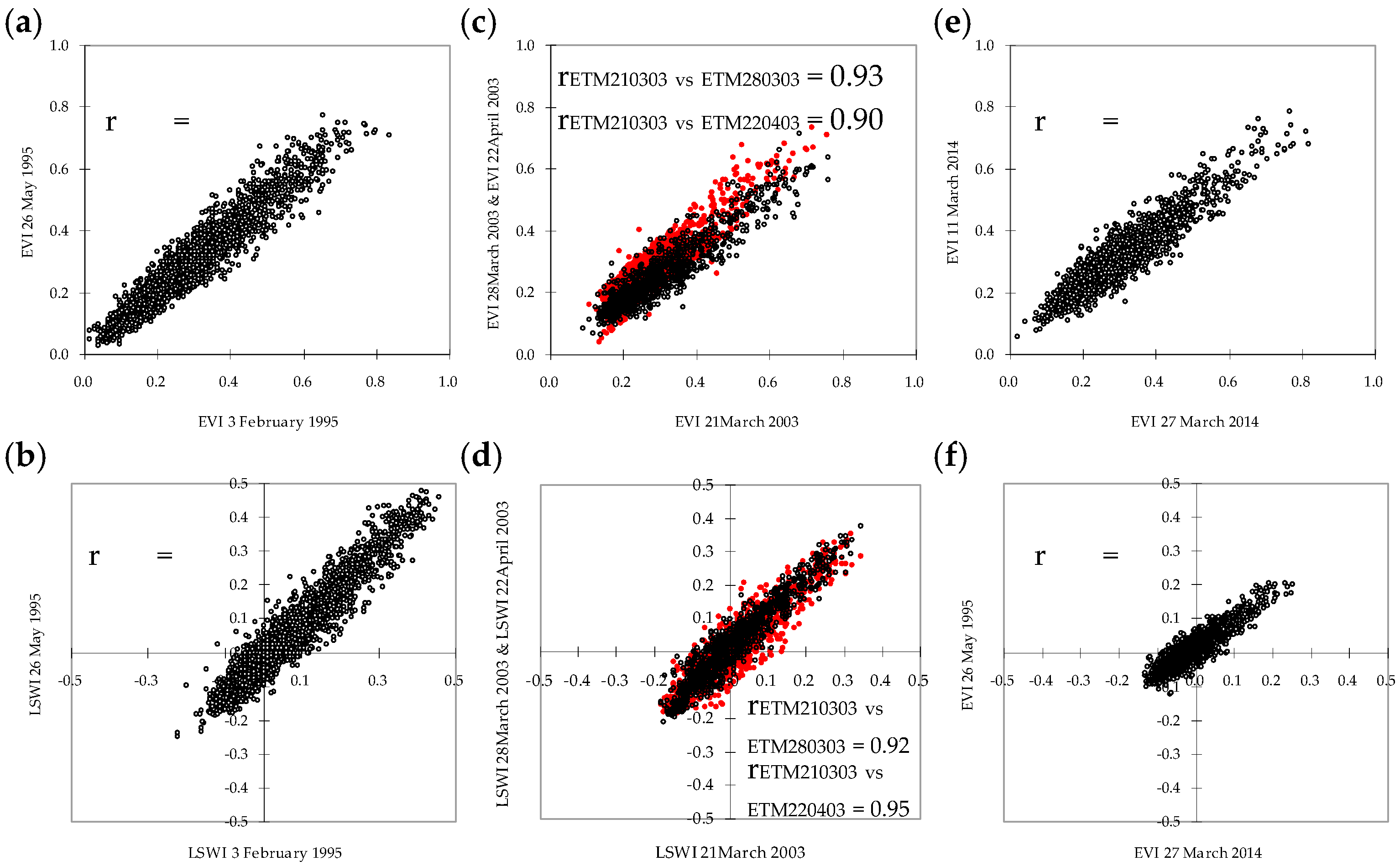
2.3. Methods
3. Results and Discussion
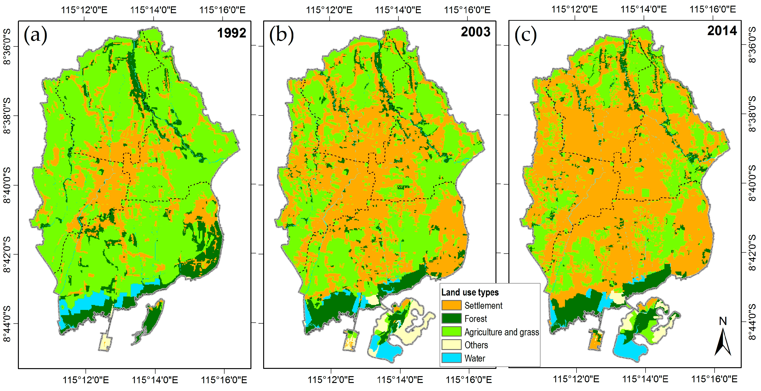
3.1. Land Use Changes
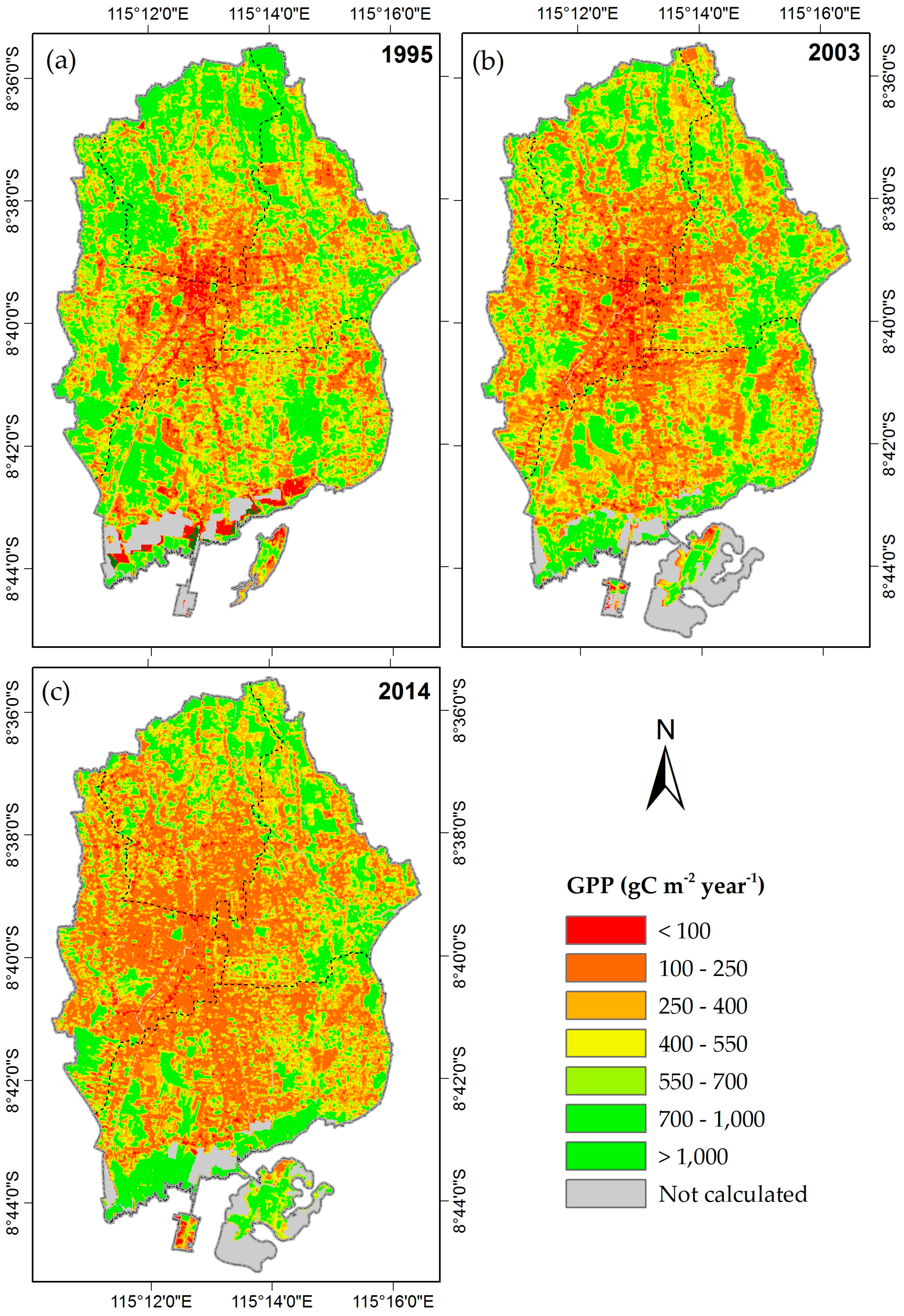
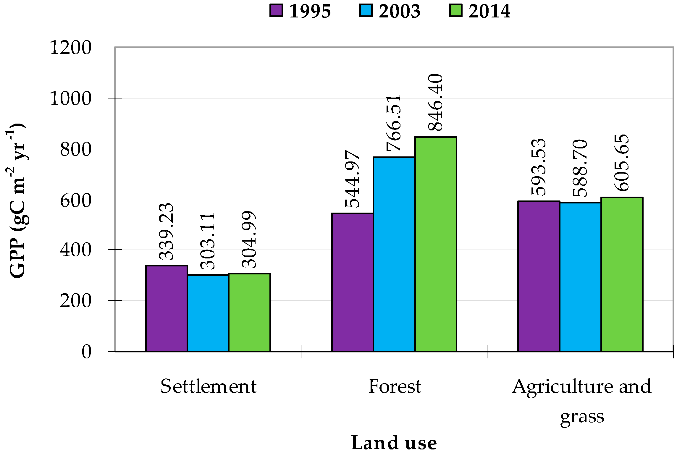
3.2. Annual Changes in GPP
4. Conclusions
Acknowledgments
Author Contributions
Conflicts of Interest
References
- Foley, J.A.; DeFries, R.; Asner, G.P.; Barford, C.; Bonan, G.; Carpenter, S.R.; Chapin, F.S.; Coe, M.T.; Daily, G.C.; Gibbs, H.K.; et al. Global consequences of land use. Science 2005, 309, 570–574. [Google Scholar] [CrossRef] [PubMed]
- Hoymann, J.; Goetzke, R. Simulation and Evaluation of Urban Growth for Germany Including Climate Change Mitigation and Adaptation Measures. ISPRS Int. J. Geo-Inf. 2016, 5, 101. [Google Scholar] [CrossRef]
- Yang, L.; Xian, G.; Klaver, J.M.; Deal, B. Urban land-cover change detection through sub-pixel imperviousness mapping using remotely sensed data. Photogramm. Eng. Remote Sens. 2003, 69, 1003–1010. [Google Scholar] [CrossRef]
- Rahman, M.T. Detection of Land Use/Land Cover Changes and Urban Sprawl in Al-Khobar, Saudi Arabia: An Analysis of Multi-Temporal Remote Sensing Data. ISPRS Int. J. Geo-Inf. 2016, 5, 15. [Google Scholar] [CrossRef]
- Lu, D.; Xu, X.; Tian, H.; Moran, E.; Zhao, M.; Running, S. The effects of urbanization on net primary productivity in southeastern China. Environ. Manag. 2010, 46, 404–410. [Google Scholar] [CrossRef] [PubMed]
- Bilsborrow, R.E.; Ogendo, H.W. Population-driven changes in land use in developing countries. Ambio 1992, 21, 37–45. [Google Scholar]
- Ivanov, S.; Webster, C. Measuring the impact of tourism on economic growth. Tour. Econ. 2007, 13, 379–388. [Google Scholar] [CrossRef]
- Surugiu, C.; Surugiu, M.R. Is the tourism sector supportive of economic growth? Empirical evidence on Romanian tourism. Tour. Econ. 2013, 19, 115–132. [Google Scholar] [CrossRef]
- Williams, A.M.; Shaw, G. Future play: Tourism, recreation and land use. Land Use Policy 2009, 26, S326–S335. [Google Scholar] [CrossRef]
- Roth, D. Environmental sustainability and legal plurality in irrigation: The Balinese subak. Curr. Opin. Environ. Sustain. 2014, 11, 1–9. [Google Scholar] [CrossRef]
- Wijaya, A.; Budiharto, R.S.; Tosiani, A.; Murdiyarso, D.; Verchot, L.V. Assessment of large scale land cover change classifications and drivers of deforestation in Indonesia. ISPRS Arch. 2015, 40, 557. [Google Scholar] [CrossRef]
- Ramdani, F.; Putra, A.P.; Utomo, B.N. Historical Urban Land Use Transformation in Virtual Geo-Library. ISPRS Int. J. Geo-Inf. 2015, 4, 1500–1511. [Google Scholar] [CrossRef]
- Kunu, P.J.; Lelolterry, H. Penggunaan Lahan dan Evolusi Penggunaan Lahan di Provinsi DKI Jakarta. J. Agroforestr. 2010, 4, 203–2007. [Google Scholar]
- As-syakur, A.R. Perubahan penggunaan lahan di Provinsi Bali. Ecotrophic J. Environ. Sci. 2011, 6, 1–7. [Google Scholar]
- Chen, T.; Huang, Q.; Liu, M.; Li, M.; Qu, L.; Deng, S.; Chen, D. Decreasing Net Primary Productivity in Response to Urbanization in Liaoning Province, China. Sustainability 2017, 9, 162. [Google Scholar] [CrossRef]
- Kalnay, E.; Cai, M. Impact of urbanization and land-use change on climate. Nature 2003, 423, 528–531. [Google Scholar] [CrossRef] [PubMed]
- Nie, W.; Yuan, Y.; Kepner, W.; Nash, M.S.; Jackson, M.; Erickson, C. Assessing impacts of landuse and landcover changes on hydrology for the upper San Pedro watershed. J. Hydrol. 2011, 407, 105–114. [Google Scholar] [CrossRef]
- Poschlod, P.; Bakker, J.P.; Kahmen, S. Changing land use and its impact on biodiversity. Basic Appl. Ecol. 2005, 6, 93–98. [Google Scholar] [CrossRef]
- Zhao, T.; Brown, D.G.; Fang, H.; Theobald, D.M.; Liu, T.; Zhang, T. Vegetation productivity consequences of human settlement growth in the eastern united states. Landsc. Ecol. 2012, 27, 1149–1165. [Google Scholar] [CrossRef]
- Hutyra, L.R.; Yoon, B.; Alberti, M. Terrestrial carbon stocks across a gradient of urbanization: A study of the Seattle, WA region. Glob. Chang. Biol. 2011, 17, 783–797. [Google Scholar] [CrossRef]
- Yan, Y.; Zhang, C.; Hu, Y.; Kuang, W. Urban Land-Cover Change and Its Impact on the Ecosystem Carbon Storage in a Dryland City. Remote Sens. 2016, 8, 6. [Google Scholar] [CrossRef]
- Wang, X.; Ma, M.; Huang, G.; Veroustraete, F.; Zhang, Z.; Song, Y.; Tan, J. Vegetation primary production estimation at maize and alpine meadow over the Heihe River Basin, China. Int. J. Appl. Earth Obs. Geoinf. 2012, 17, 94–101. [Google Scholar] [CrossRef]
- Wagle, P.; Xiao, X.; Torn, M.S.; Cook, D.R.; Matamala, R.; Fischer, M.L.; Jin, C.; Dong, J.; Biradar, C. Sensitivity of vegetation indices and gross primary production of tallgrass prairie to severe drought. Remote Sens. Environ. 2014, 152, 1–14. [Google Scholar] [CrossRef]
- Nemani, R.R.; Keeling, C.D.; Hashimoto, H.; Jolly, W.M.; Piper, S.C.; Tucker, C.J.; Myneni, R.B.; Running, S.W. Climate-driven increases in global terrestrial net primary production from 1982 to 1999. Science 2003, 300, 1560–1563. [Google Scholar] [CrossRef] [PubMed]
- Zhao, T.; Brown, D.G.; Bergen, K.M. Increasing gross primary production (GPP) in the urbanizing landscapes of southeastern Michigan. Photogramm. Eng. Remote Sens. 2007, 73, 1159–1167. [Google Scholar] [CrossRef]
- Wu, C.Y.; Gonsamo, A.; Zhang, F.M.; Chen, J.M. The potential of the greenness and radiation (GR) model to interpret 8-day gross primary production of vegetation. ISPRS J. Photogramm. Remote Sens. 2014, 88, 69–79. [Google Scholar] [CrossRef]
- Inoue, Y.; Peñuelas, J.; Miyata, A.; Mano, M. Normalized difference spectral indices for estimating photosynthetic hyperspectral and CO2 flux measurements in rice. Remote Sens. Environ. 2008, 112, 156–172. [Google Scholar] [CrossRef]
- Turner, D.P.; Gowerb, S.T.; Cohenc, W.B.; Gregorya, M.; Maiersperger, T.K. Effects of spatial variability in light use efficiency on Satellite-Based NPP monitoring. Remote Sens. Environ. 2002, 80, 397–405. [Google Scholar] [CrossRef]
- Myneni, R.B.; Williams, D.L. On the relationship between FAPAR and NDVI. Remote Sens. Environ. 1994, 49, 200–211. [Google Scholar] [CrossRef]
- Iwata, H.; Ueyama, M.; Iwama, C.; Harazono, Y. Variations in fraction of absorbed photosynthetically active radiation and comparisons with MODIS data in burned black spruce forests of Interior Alaska. Pol. Sci. 2013, 7, 113–124. [Google Scholar] [CrossRef]
- Green, K.; Kempka, D.; Lackey, L. Using remote sensing to detect and monitor land-cover and land-use change. Photogramm. Eng. Remote Sens. 1994, 60, 331–337. [Google Scholar]
- Rogan, J.; Chen, D. Remote sensing technology for mapping and monitoring land-cover and land-use change. Prog. Plan. 2004, 61, 301–325. [Google Scholar] [CrossRef]
- Gómez, C.; White, J.C.; Wulder, M.A. Optical remotely sensed time series data for land cover classification: A review. ISPRS J. Photogramm. Remote Sens. 2016, 116, 55–72. [Google Scholar] [CrossRef]
- Turner, D.P.; Ritts, W.D.; Cohen, W.B.; Gower, S.T.; Zhao, M.; Running, S.W.; Wofsy, S.C.; Urbanski, S.; Dunn, A.L.; Munger, J.W. Scaling gross primary production (GPP) over boreal and deciduous forest landscapes in support of MODIS GPP product validation. Remote Sens. Environ. 2003, 88, 256–270. [Google Scholar] [CrossRef]
- Gitelson, A.A.; Peng, Y.; Masek, J.G.; Rundquist, D.C.; Verma, S.; Suyker, A.; Baker, J.M.; Hatfield, J.L.; Meyers, T. Remote estimation of crop gross primary production with Landsat data. Remote Sens. Environ. 2012, 121, 404–414. [Google Scholar] [CrossRef]
- Chapin, F.S., III; Matson, P.A.; Vitousek, P. Principles of Terrestrial Ecosystem Ecology, 2nd ed.; Springer: New York, NY, USA, 2011. [Google Scholar]
- Yuan, W.; Cai, W.; Liu, S.; Dong, W.; Chen, J.; Arain, M.A.; Blanken, P.D.; Cescatti, A.; Wohlfahrt, G.; Georgiadis, T.; et al. Vegetation-specific model parameters are not required for estimating gross primary production. Ecol. Model. 2014, 292, 1–10. [Google Scholar] [CrossRef]
- Sims, D.A.; Luo, H.; Hastings, S.; Oechel, W.C.; Rahman, A.F.; Gamon, J.A. Parallel adjustments in vegetation greenness and ecosystem CO2 exchange in response to drought in a southern California chaparral ecosystem. Remote Sens. Environ. 2006, 103, 289–303. [Google Scholar] [CrossRef]
- Xiao, X.; Hollinger, D.; Aber, J.; Goltz, M.; Zhang, Q. Satellite-based modeling of gross primary production in an evergreen needle leaf forest. Remote Sens. Environ. 2004, 89, 519–534. [Google Scholar] [CrossRef]
- Xiao, X.; Zhang, Q.; Saleska, S.; Hutyra, L.; de Camargo, P.; Wofsy, S.; Frolking, S.; Boles, S.; Keller, M.; Moore, B. Satellite-based modeling of Gross Primary Production in a seasonally moist tropical evergreen forest. Remote Sens. Environ. 2005, 94, 105–122. [Google Scholar] [CrossRef]
- Madugundu, R.; Al-Gaadi, K.A.; Tola, E.; Kayad, A.G.; Jha, C.S. Estimation of gross primary production of irrigated maize using Landsat-8 imagery and Eddy Covariance data. Saudi J. Biol. Sci. 2017, 24, 410–420. [Google Scholar] [CrossRef] [PubMed]
- Danelichen, V.H.; Biudes, M.S.; Velasque, M.; Machado, N.G.; Gomes, R.S.; Vourlitis, G.L.; Nogueira, J.S. Estimating of gross primary production in an Amazon-Cerrado transitional forest using MODIS and Landsat imagery. An. Acad. Bras. Cienc. 2015, 87, 1545–1564. [Google Scholar] [CrossRef] [PubMed]
- Vetrita, Y.; Chaoyang, W.; Zheng, N.; Hirano, T. Evaluation of light use efficiency model using modis in tropical peat swamp forest, Indonesia. In Proceedings of the Second CReSOS International Symposium on Southeast Asia Environmental Problems and Satellite Remote Sensing, Bali, Indonesia, 21–22 February 2011; pp. 127–134. [Google Scholar]
- As-syakur, A.R.; Tanaka, T.; Osawa, T.; Mahendra, M.S. Indonesian rainfall variability observation using TRMM multi-satellite data. Int. J. Remote Sens. 2013, 34, 7723–7738. [Google Scholar] [CrossRef]
- Aldrian, E.; Susanto, D.R. Identification of three dominant rainfall regions within Indonesia and their relationship to sea surface temperature. Int. J. Climatol. 2003, 23, 1435–1452. [Google Scholar] [CrossRef]
- As-syakur, A.R.; Osawa, T.; Adnyana, I.W.S. Medium Spatial Resolution Satellite Imagery to Estimate Gross Primary Production in an Urban Area. Remote Sens. 2010, 2, 1496–1507. [Google Scholar] [CrossRef]
- Davis, A.; Marshak, A.; Cahalan, R.; Wiscombe, W. The Landsat scale break in stratocumulus as a three-dimensional radiative transfer effect: Implications for cloud remote sensing. J. Atmos. Sci. 1997, 54, 241–260. [Google Scholar] [CrossRef]
- Goodwin, N.R.; Collett, L.J.; Denham, R.J.; Flood, N.; Tindall, D. Cloud and cloud shadow screening across Queensland, Australia: An automated method for Landsat TM/ETM+ time series. Remote Sens. Environ. 2013, 134, 50–65. [Google Scholar] [CrossRef]
- Zhu, Z.; Woodcock, C.E. Object-based cloud and cloud shadow detection in Landsat imagery. Remote Sens. Environ. 2012, 118, 83–94. [Google Scholar] [CrossRef]
- Irish, R.R.; Barker, J.L.; Goward, S.N.; Arvidson, T. Characterization of the Landsat-7 ETM+ automated cloud-cover assessment (ACCA) algorithm. Photogramm. Eng. Remote Sens. 2006, 72, 1179–1188. [Google Scholar] [CrossRef]
- Liu, H.Q.; Huete, A.R. A feedback based modification of the NDV I to minimize canopy background and atmospheric noise. IEEE Trans. Geosci. Remote Sens. 1995, 33, 457–465. [Google Scholar]
- Huete, A.R.; Liu, H.Q.; Batchily, K.; Van Leeuwen, W.J.D.A. A comparison of vegetation indices over a global set of TM images for EOS-MODIS. Remote Sens. Environ. 1997, 59, 440–451. [Google Scholar] [CrossRef]
- Xiao, X.; Boles, S.; Frolking, S.; Salas, W.; Moore, B., III; Li, C.; He, L.; Zhao, R. Observation of flooding and rice transplanting of paddy rice fields at the site to landscape scales in China using VEGETATION sensor data. Int. J. Remote Sens. 2002, 23, 3009–3022. [Google Scholar] [CrossRef]
- Japan International Cooperation Agency (JICA). The Comprehensive Study on Water Resources Development and Management in Bali Province, in the Republic of Indonesia: Final Report; Japan International Cooperation Agency and Directorate General of Water Resources, Indonesian Ministry of Public Works: Jakarta, Indonesia, 2006.
- Hirano, T.; Segah, H.; Harada, T.; Limin, S.; June, T.; Hirata, R.; Osaki, M. Carbon dioxide balance of a tropical peat swamp forest in Kalimantan, Indonesia. Glob. Chang. Biol. 2007, 13, 412–425. [Google Scholar] [CrossRef]
- Raich, J.W.; Rastetter, E.B.; Melillo, J.M.; Kicklighter, D.W.; Steudler, P.A.; Peterson, B.J.; Grace, A.L.; Moore, B.; Vorosmarty, C.J. Potential net primary productivity in South America: Application of a global model. Ecol. Appl. 1991, 1, 399–429. [Google Scholar] [CrossRef] [PubMed]
- Nguy-Robertson, A.; Suyker, A.; Xiao, X. Modeling gross primary production of maize and soybean croplands using light quality, temperature, water stress, and phenology. Agric. For. Meteorol. 2015, 213, 160–172. [Google Scholar] [CrossRef]
- Kalfas, J.L.; Xiao, X.; Vanegas, D.X.; Verma, S.B.; Suyker, A.E. Modeling gross primary production of irrigated and rain-fed maize using MODIS imagery and CO2 flux tower data. Agric. For. Meteorol. 2011, 151, 1514–1528. [Google Scholar] [CrossRef]
- Jacovides, C.; Tymvios, F.; Asimakopoulos, D.; Theofilou, K.; Pashiardes, S. Global photosynthetically active radiation and its relationship with global solar radiation in the Eastern Mediterranean basin. Theor. Appl. Climatol. 2003, 74, 227–233. [Google Scholar] [CrossRef]
- Rao, C.N. Photosynthetically active components of global solar radiation: Measurements and model computations. Arch. Meteorol. Geophys. B 1984, 34, 353–364. [Google Scholar]
- González, J.A.; Calbó, J. Modelled and measured ratio of PAR to global radiation under cloudless skies. Agric. For. Meteorol. 2002, 110, 319–325. [Google Scholar] [CrossRef]
- Escobedo, J.F.; Gomes, E.N.; Oliveira, A.P.; Soares, J. Ratios of UV, PAR and NIR components to global solar radiation measured at Botucatu site in Brazil. Renew. Energy 2011, 36, 169–178. [Google Scholar] [CrossRef]
- Jin, C.; Xiao, X.; Wagle, P.; Griffis, T.; Dong, J.; Wu, C.; Qin, Y.; Cook, D.R. Effects of in-situ and reanalysis climate data on estimation of cropland gross primary production using the Vegetation Photosynthesis Model. Agric. For. Meteorol. 2015, 213, 240–250. [Google Scholar] [CrossRef]
- Halawa, E.E.H.; Sugiyatno, S. Estimation of global solar radiation in the Indonesian climatic region. Renew. Energy 2001, 24, 197–206. [Google Scholar] [CrossRef]
- As-syakur, A.R.; Osawa, T.; Miura, F.; Nuarsa, I.W.; Ekayanti, N.W.; Dharma, I.G.B.S.; Adnyana, I.W.S.; Arthana, I.W.; Tanaka, T. Maritime Continent rainfall variability during the TRMM era: The role of monsoon, topography and El Niño Modoki. Dyn. Atmos. Oceans. 2016, 75, 58–77. [Google Scholar] [CrossRef]
- Nuarsa, I.W.; Nishio, F.; Hongo, C.; Mahardika, I.G. Using variance analysis of multitemporal MODIS images for rice field mapping in Bali Province, Indonesia. Int. J. Remote Sens. 2012, 33, 5402–5417. [Google Scholar] [CrossRef]
- Takama, T.; Setyani, P.; Aldrian, E. Climate change vulnerability to rice paddy production in Bali, Indonesia. In Handbook of Climate Change Adaptation; Filho, W.L., Ed.; Springer: Berlin/Heidelberg, Germany, 2015; pp. 1731–1757. ISBN 978-3-642-38669-5. [Google Scholar]
- Jayanti, I.A.G.K.; Osawa, T.; Adnyana, I.W.S.; Tanaka, T.; Nuarsa, I.W.; As-syakur, A.R. Multitemporal MODIS Data to Mapping Rice Field Distribution in Bali Province of Indonesia Based on the Temporal Dynamic Characteristics of the Rice Plant. Earth Sci. Res. 2012, 1, 64–74. [Google Scholar]
- As-syakur, A.R.; Nuarsa, I.W.; Osawa, T. Impacts of El Niño on agricultural drought in Bali, Indonesia. In Proceedings of the 19th Symposium on Remote Sensing for Environment, Chiba, Japan, 16 February 2017; p. 54. [Google Scholar]
- Stevenson, N.J.; Lewis, R.R.; Burbridge, P.R. Disused shrimp ponds and mangrove rehabilitation. In An International Perspective on Wetland Rehabilitation; Streever, W.J., Ed.; Springer: Dordrecht, The Netherlands, 1999; pp. 277–297. ISBN 978-94-011-4683-8. [Google Scholar]
- Kytzia, S.; Walz, A.; Wegmann, M. How can tourism use land more efficiently? A model–based approach to land–use efficiency for tourist destinations. Tour. Manag. 2011, 32, 629–640. [Google Scholar] [CrossRef]
- Xi, J.; Zhao, M.; Ge, Q.; Kong, Q. Changes in land use of a village driven by over 25 years of tourism: The case of Gougezhuang village, China. Land Use Policy 2014, 40, 119–130. [Google Scholar] [CrossRef]
- Mao, X.; Meng, J.; Wang, Q. Modeling the effects of tourism and land regulation on land-use change in tourist regions: A case study of the Lijiang River Basin in Guilin, China. Land Use Policy 2014, 41, 368–377. [Google Scholar] [CrossRef]
- Wu, Q.; Li, H.Q.; Wang, R.S.; Paulussen, J.; He, Y.; Wang, M.; Wang, B.H.; Wang, Z. Monitoring and predicting land use change in Beijing using remote sensing and GIS. Landsc. Urban Plan. 2006, 78, 322–333. [Google Scholar] [CrossRef]
- Howe, L. The Changing World of Bali: Religion, Society and Tourism; Routledge: New York, NY, USA, 2006. [Google Scholar]
- Lorenzen, S.; Lorenzen, R.P. A Case Study of Balinese Irrigation Management: Institutional Dynamics and Challenges. In Proceedings of the Second Southeast Asia Water Forum, Bali, Indonesia, 29 August–3 September 2005. [Google Scholar]
- Pitana, I.G. Tri Hita Karana–The Local Wisdom of the Balinese in Managing Development. In Trends and Issues in Global Tourism 2010; Conrady, R., Buck, M., Eds.; Springer: Berlin/Heidelberg, Germany, 2010; pp. 139–150. ISBN 978-3-642-10829-7. [Google Scholar]
- Lambin, E.F.; Turner, B.L.; Geist, H.J.; Agbola, S.B.; Angelsen, A.; Bruce, J.W.; Coomes, O.T.; Dirzo, R.; Fischer, G.; Folke, C.; et al. The causes of land-use and land-cover change: Moving beyond the myths. Glob. Environ. Chang. Part A Hum. Policy Dimens. 2001, 11, 261–269. [Google Scholar] [CrossRef]
- Parker, D.C.; Manson, S.M.; Janssen, M.A.; Hoffmann, M.J.; Deadman, P. Multi-Agent Systems for the simulation of land-use and land-cover change: A review. Ann. Assoc. Am. Geogr. 2003, 93, 314–337. [Google Scholar] [CrossRef]
- Wu, X.; Shen, Z.; Liu, R.; Ding, X. Land Use/Cover Dynamics in Response to Changes in Environmental and Socio-Political Forces in the Upper Reaches of Yangtze River, China. Sensors 2008, 8, 8104–8122. [Google Scholar] [CrossRef] [PubMed]
- Allen, J.; Lu, K.S.; Potts, T.D. A GIS-based analysis and prediction of land-use change in a coastal tourism destination area. In Proceedings of the 1999 International Symposium on Coastal and Marine Tourism: Balancing Tourism and Conservation, Vancouver, BC, Canada, 26–29 April 1999; pp. 287–297. [Google Scholar]
- Conway, T.M.; Lathrop, R.G. Alternative land use regulations and environmental impacts: Assessing future land use in an urbanizing watershed. Landsc. Urban Plan. 2005, 71, 1–15. [Google Scholar] [CrossRef]
- Quigley, J.M.; Rosenthal, L.A. The effects of land use regulation on the price of housing: What do we know? What can we learn? Cityscape: J. Pol. Devel. Res. 2005, 8, 69–137. [Google Scholar]
- Mandelker, D.R. The role of the local comprehensive plan in land use regulation. Mich. Law Rev. 1976, 74, 899–973. [Google Scholar] [CrossRef]
- As-syakur, A.R.; Adnyana, I.W.S.; Arthana, I.W.; Nuarsa, I.W. Enhanced Built-Up and Bareness Index (EBBI) for Mapping Built-Up and Bare Land in an Urban Area. Remote Sens. 2012, 4, 2957–2970. [Google Scholar] [CrossRef]
- Yang, H.F.; Mu, S.J.; Li, J.L. Effects of ecological restoration projects on land use and land cover change and its influences on territorial NPP in Xinjiang, China. Catena 2014, 115, 85–95. [Google Scholar] [CrossRef]
- Briber, B.M.; Hutyra, L.R.; Reinmann, A.B.; Raciti, S.M.; Dearborn, V.K.; Holden, C.E.; Dunn, A.L. Tree productivity enhanced with conversion from forest to urban land covers. PLoS ONE 2015, 10, e0136237. [Google Scholar] [CrossRef] [PubMed]
- Iakovoglou, V.; Thompson, J.; Burras, L.; Kipper, R. Factors related to tree growth across urban-rural gradients in the Midwest, USA. Urban Ecosyst. 2001, 5, 71–85. [Google Scholar] [CrossRef]
- MCDonald, R.I.; Urban, D.L. Forest edges and tree growth rates in the North Carolina Piedmont. Ecology 2004, 85, 2258–2266. [Google Scholar] [CrossRef]
- Donato, D.C.; Kauffman, J.B.; Murdiyarso, D.; Kurnianto, S.; Stidham, M.; Kanninen, M. Mangroves among the most carbon-rich forests in the tropics. Nat. Geosci. 2011, 4, 293–297. [Google Scholar] [CrossRef]
- Duarte, C.M.; Middelburg, J.J.; Caraco, N. Major role of marine vegetation on the oceanic carbon cycle. Biogeosciences 2005, 2, 1–8. [Google Scholar] [CrossRef]
- Cohen, W.B.; Yang, Z.; Kennedy, R. Detecting trends in forest disturbance and recovery using yearly Landsat time series: 2. TimeSync—Tools for calibration and validation. Remote Sens. Environ. 2010, 114, 2911–2924. [Google Scholar] [CrossRef]
- Schneider, A. Monitoring land cover change in urban and peri-urban areas using dense time stacks of Landsat satellite data and a data mining approach. Remote Sens. Environ. 2012, 124, 689–704. [Google Scholar] [CrossRef]
- Lee, T.; Yeh, H. Applying remote sensing techniques to monitor shifting wetland vegetation: A case study of Danshui River estuary mangrove communities, Taiwan. Ecol. Eng. 2009, 35, 487–496. [Google Scholar] [CrossRef]
- Chen, D.; Stow, D.A.; Gong, P. Examining the effect of spatial resolution and texture window size on classification accuracy: An urban environment case. Int. J. Remote Sens. 2004, 25, 2177–2192. [Google Scholar] [CrossRef]
- Rocchini, D. Effects of spatial and spectral resolution in estimating ecosystem A-diversity by satellite imagery. Remote Sens. Environ. 2007, 111, 423–434. [Google Scholar] [CrossRef]
- Cui, Y.; Xiao, X.; Zhang, Y.; Dong, J.; Qin, Y.; Doughty, R.B.; Zhang, G.; Wang, J.; Wu, X.; Qin, Y.; et al. Temporal consistency between gross primary production and solar-induced chlorophyll fluorescence in the ten most populous megacity areas over years. Sci. Rep. 2017, 7, 14963. [Google Scholar] [CrossRef] [PubMed]
- Churkina, G. Modeling the carbon cycle of urban systems. Ecol. Modell. 2008, 216, 107–113. [Google Scholar] [CrossRef]
- Chowdhury, R.R.; Larson, K.; Grove, M.; Polsky, C.; Cook, E.; Onsted, J.; Ogden, L. A multi-scalar approach to theorizing socio-ecological dynamics of urban residential landscapes. Cities Environ. 2011, 4, 6. [Google Scholar] [CrossRef]
- Stewart, I.D.; Oke, T.R. Local climate zones for urban temperature studies. Bull. Am. Meteorol. Soc. 2012, 93, 1879–1900. [Google Scholar] [CrossRef]


| Land Use | Description |
|---|---|
| Settlement | Combines built-up areas, roads, backyards, and parking |
| Forest | Combines mangroves, perennial plants, and shrubland |
| Agriculture and grass | Combines agricultural farmlands (irrigated paddy fields), dry land, grassy fields, golf courses, and parks |
| Others | Combines bare land and sand |
| Water | Combines rivers, fishponds, and dams |
| Land use | 1992 | 2003 | 2014 | |||
|---|---|---|---|---|---|---|
| Area (ha) | % | Area (ha) | % | Area (ha) | % | |
| Settlement | 2396.34 | 19.89% | 5421.87 | 43.49% | 7302.78 | 58.57% |
| Forest | 1382.94 | 11.48% | 1226.43 | 9.84% | 1207.53 | 9.68% |
| Agriculture and grass | 7868.07 | 65.31% | 5239.98 | 42.03% | 3517.56 | 28.21% |
| Others | 62.55 | 0.52% | 359.55 | 2.88% | 210.06 | 1.68% |
| Water | 337.32 | 2.80% | 220.23 | 1.77% | 230.13 | 1.85% |
| Total | 12,047.22 | 12,468.06 | 12,468.06 | |||
| Land Use | 1992 to 2003 | 2003 to 2014 | 1992 to 2014 | |||
|---|---|---|---|---|---|---|
| Changes | LUEI (% year−1) | Changes | LUEI (% year−1) | Changes | LUEI (% year−1) | |
| Settlement | 126.26% | 10.52% | 34.69% | 2.89% | 204.75% | 10.24% |
| Forest | −11.32% | −0.94% | −1.54% | −0.13% | −12.68% | −0.63% |
| Agriculture and grass | −33.40% | −2.78% | −32.87% | −2.74% | −55.29% | −2.76% |
| Others | 474.82% | 39.57% | −41.58% | −3.46% | 235.83% | 11.79% |
| Water | −34.71% | −2.89% | 4.50% | 0.37% | −31.78% | −1.59% |
| Land use | 1995 | 2003 | 2014 | |||
|---|---|---|---|---|---|---|
| Total | % | Total | % | Total | % | |
| Settlement | 7102.04 | 11.53% | 15,607.49 | 28.06% | 22,274.93 | 41.39% |
| Forest | 8071.18 | 13.10% | 9238.85 | 16.61% | 10,268.58 | 19.08% |
| Agriculture and grass | 46,435.93 | 75.37% | 30,775.48 | 55.33% | 21,271.68 | 39.53% |
| Total | 61,609.15 | 55,621.81 | 53,815.19 | |||
| Land Use | 1995 to 2003 | 2003 to 2014 | 1995 to 2014 |
|---|---|---|---|
| Settlement | 119.76% | 42.72% | 213.64% |
| Forest | 14.47% | 11.15% | 27.23% |
| Agriculture and grass | −33.72% | −30.88% | −54.19% |
| Total | −9.72% | −3.25% | −12.65% |
| Land Use | 1995 to 2003 | 2003 to 2014 | 1995 to 2014 |
|---|---|---|---|
| Settlement | 13.31% | 3.56% | 10.68% |
| Forest | 1.61% | 0.93% | 1.36% |
| Agriculture and grass | −3.75% | −2.57% | −2.71% |
| Total | −1.08% | −0.27% | −0.63% |
© 2018 by the authors. Licensee MDPI, Basel, Switzerland. This article is an open access article distributed under the terms and conditions of the Creative Commons Attribution (CC BY) license (http://creativecommons.org/licenses/by/4.0/).
Share and Cite
Nuarsa, I.W.; As-syakur, A.R.; Gunadi, I.G.A.; Sukewijaya, I.M. Changes in Gross Primary Production (GPP) over the Past Two Decades Due to Land Use Conversion in a Tourism City. ISPRS Int. J. Geo-Inf. 2018, 7, 57. https://doi.org/10.3390/ijgi7020057
Nuarsa IW, As-syakur AR, Gunadi IGA, Sukewijaya IM. Changes in Gross Primary Production (GPP) over the Past Two Decades Due to Land Use Conversion in a Tourism City. ISPRS International Journal of Geo-Information. 2018; 7(2):57. https://doi.org/10.3390/ijgi7020057
Chicago/Turabian StyleNuarsa, I Wayan, Abd. Rahman As-syakur, I Gusti Alit Gunadi, and I Made Sukewijaya. 2018. "Changes in Gross Primary Production (GPP) over the Past Two Decades Due to Land Use Conversion in a Tourism City" ISPRS International Journal of Geo-Information 7, no. 2: 57. https://doi.org/10.3390/ijgi7020057
APA StyleNuarsa, I. W., As-syakur, A. R., Gunadi, I. G. A., & Sukewijaya, I. M. (2018). Changes in Gross Primary Production (GPP) over the Past Two Decades Due to Land Use Conversion in a Tourism City. ISPRS International Journal of Geo-Information, 7(2), 57. https://doi.org/10.3390/ijgi7020057