Pixel-Wise Classification Method for High Resolution Remote Sensing Imagery Using Deep Neural Networks

Abstract

Considering the classification of high spatial resolution remote sensing imagery, this paper presents a novel classification method for such imagery using deep neural networks. Deep learning methods, such as a fully convolutional network (FCN) model, achieve state-of-the-art performance in natural image semantic segmentation when provided with large-scale datasets and respective labels. To use data efficiently in the training stage, we first pre-segment training images and their labels into small patches as supplements of training data using graph-based segmentation and the selective search method. Subsequently, FCN with atrous convolution is used to perform pixel-wise classification. In the testing stage, post-processing with fully connected conditional random fields (CRFs) is used to refine results. Extensive experiments based on the Vaihingen dataset demonstrate that our method performs better than the reference state-of-the-art networks when applied to high-resolution remote sensing imagery classification.

1. Introduction

Pixel-wise classification is a fundamental task in remote sensing that aims at assigning a semantic class, e.g., vegetation, buildings, vehicles or roads, accurately to every individual pixel of an image. As a pattern recognition problem, pixel-wise classification has drawn significant attention for several decades, with many aspects yet to be resolved. Such pixel-level cluster and classification methods, as k-means [1], neural networks [2,3], support vector machines [4,5], random forest [6,7] and boosting [8], are widely used to classify low spatial resolution (10–30 m) images. However, at a higher resolution of both spectral and spatial remote sensing imagery, the above methods are sensitive to noise, lack semantic meaning of objects, and cannot be easily used to acquire object-level information.

High resolution (2 m and higher spatial resolution) remote sensing imagery contains more small objects and fine details; thus, it is more meaningful to recognize a ground object, rather than pixels, in a high spatial resolution image. Commercial software programs such as eCognition [9] and ENVI [10] have implemented object-based image classification methods that allow for the combined use of spatial and contextual features in addition to spectral information and can achieve a higher classification accuracy in certain situations. Considering the complexity of land cover that contains vegetation, water, soil and other physical land features, including those created solely by human activities, it is still challenging for object-oriented approaches to improve classification accuracy.

Traditionally, classification of remote sensing imagery focused on two steps, i.e., feature extraction methods and supervised learning algorithms. Various methods have been proposed to extract features using hand-crafted descriptors, such as Scale-Invariant Feature Transform (SIFT) [11] and Histogram of Oriented Gradients (HOG) [12]. However, the two steps mentioned above are typically viewed as distinct approaches. Convolutional neural networks (CNNs) combine the two steps into one network that learns contextual features at different scales and computes the score of each class at the end of the network. Another benefit of CNNs is that they can be trained to optimize all weights in the network using an efficient weight update technique such as stochastic gradient descent (SGD) [13] end-to-end. Although CNNs have achieved remarkable results in image categorization, they do not consider pixel-wise semantic classification. In image categorization, the input of a network is an image, while the goal is to predict the correct category of the entire image. FCN [14]-based models have been successfully applied to natural image semantic segmentation and are currently the state-of-the-art for PASCAL VOC datasets [15]. However, FCN models do not take into account relations between pixels and ignore the spatial regularity in the usual pixel-wise classification method. In addition, the vast majority of research focuses on optimization of the network structure without considering efficient use of labeled data that is very important to deep neural networks.

To overcome the above challenges, in this paper, we introduce a novel pipeline for pixel-wise classification of high-resolution remote sensing imagery. Our method consists of three parts: training data augmentation in the training stage, supervised classification approach based on an atrous spatial pyramid pooling (ASPP) network, and post-processing that uses fully connected CRFs to generate the final refined classification result in the testing stage. Compared to existing methods, our novel contributions are as follows:

• We specifically propose applying data augmentation in the training stage of supervised classification approach, which could systematically improve classification accuracy.
• We apply a supervised classification approach based on an ASPP network to high spatial resolution remote sensing imagery, following the procedure of Chen et al. [16].
• We compare our approach to the basic FCN and FCN-8s approaches proposed in [14], the multi-layer perceptron (MLP) approach proposed in [17,18] and the ASPP approach of [16] that successfully performed high-resolution remote sensing imagery classification and natural image segmentation.

2. Related Work

Over the last few years, methods based on deep learning for computer vision applications, such as object detection and semantic segmentation, represented the state-of-the-art. Since the deep learning theory was explicitly proposed by Hinton et al. [19] in 2006, various deep learning architectures, such as Deep Belief Networks (DBNs) [20], Stacked AutoEncoder (SAE) [21], Convolutional Neural Networks (CNNs) [22], and Recurrent Neural Networks (RNN) [23], have been introduced to computer vision [24,25], speech recognition, natural language processing and audio recognition. CNN, the most popular deep learning method in computer vision, is used to learn the features of images via an architecture of connected layers and neural networks.

Pixel-wise classification is an active research topic, stimulated by challenging datasets, e.g., PASCAL [15] and MS-COCO [26]. Long et al. [14] proposed the Fully Convolutional Network (FCN) based on the standard CNN. By replacing fully connected layers in a CNN with convolutional layers, the FCN maintains a 2D structure of feature maps and was the first to implement CNN-based image semantic segmentation. SegNet [27] introduced an encoder and decoder network into the pooling indices. The encoder network is topologically identical to convolutional layers in VGG16 [28], while the fully connected layers of VGG16 are removed, making the SegNet encoder network significantly smaller and easier to train. Yu [29] proposed a new convolutional network designed for dense prediction using dilated convolutions to systematically aggregate multi-scale contextual information and support an exponential expansion of the receptive field without losing resolution. CRF-RNN [30] combined the strengths of CNNs and CRF-based probabilistic graphical modeling in a single framework. It can refine coarse outputs from a traditional CNN both forwards and backwards by proposing mean-field approximate inference for the dense CRF with Gaussian pairwise potentials as a recurrent neural network (RNN) [31,32]. RefineNet [33] combined rough high-level semantic features and fine-grained low-level features. All components of RefineNet used residual connections with identity mappings, such that gradients could be directly propagated through short-range and long-range residual connections. However, training the entire network was too time-consuming. Large Kernel Matters [34] proposed a global convolutional network to address both classification and localization challenges of semantic segmentation using a large kernel and an effective receptive field. PSPNet [35] proposed a pyramid scene parsing network to exploit the global context information of an image at different region scales, and subsequently harvested different sub-region representations. PSPNet concatenated the regular CNN layers and the upsampled pyramid pooling layers, carrying both local and global context information to the image. However, the results were highly dependent on pre-trained model parameters. LargeFOV [36] and ASPP [16] combined the responses at the final CNN layer with fully connected CRFs to localize the segment boundaries, achieving a higher accuracy than previous methods.

In remote sensing research, deep learning has recently been introduced into high-resolution and hyperspectral data [37] classification. Mnih [38] proposed an efficient large-scale patch-based learning approach to road detection by initializing the feature detectors using RBMs (Restricted Boltzmann Machines). Basu [39] presented a framework for classification of satellite imagery that extracted features and fed normalized feature vectors to a DBN for classification. Basu [40] presented a framework using the statistical region merging (SRM) algorithm for segmentation, neural networks for classification and CRF for the result refinement to estimate tree cover for the entirety of the continental United States. Since Penatti et al. [41] showed that a pre-trained CNN used to recognize natural image objects generalizes well to categorizing remote sensing data by transfer learning, and CNN-based methods became increasingly popular in a remote sensing research. On the basis of patch-based CNN classification [42], Volpi [43] presented a CNN-based system relying on a downsample-then-upsample architecture. Specifically, it first learned a rough spatial map of high-level representations using convolutions and subsequently learned to upsample them back to the original resolution using deconvolutions. Based on SegNet [27], Yu Liu [44] proposed an hourglass-shaped network (HSN) for high-resolution aerial imagery that featured multi-scale inference by using inception modules replacing simple convolutional layers and forwarding information from the encoding layers directly to decoding ones by skip connections. In addition, also based on SegNet [27], Nicolas Audebert [45] presented a deep learning-based segment-before-detect method for the subsequent detection and classification of several varieties of wheeled vehicles in high-resolution remote sensing imagery. Based on FCN [14] and MLP [17,18], a CNN framework was derived to learn features at different resolutions and apply a simple method for combining such features. Similarly, to LargeFOV [36], Gang Fu [46] designed a multi-scale network architecture by adding a skip-layer structure to multi-resolution image classification of GF-2 images. Marmanis [47,48] extracted scale-dependent class boundaries before each pooling level, with the class boundaries fused into the final multi-scale boundary prediction. Along with ensemble learning, the model showed very high accuracy on the Vaihingen dataset.

Nevertheless, the tendency of the network structure is to extract the global context information of an image from different region scales. We summarize the related work and compare various models in

Table 1. A summary of related work.

Network Architecture	Summary
RBM, DBN [39]	Unsupervised learning methods for feature extraction.
Patch-Based CNN [42,43]	The first CNN-based model for pixel-wise image classification; however, it suffered from low accuracy.
FCN [14,17,18,47,48]	The first pixel-wise classification method by an improved end-to-end CNN model; however, its results were coarse.
SegNet [27,44,45]	Achieved a higher accuracy than FCN, yet lower than that of Atrous Convolution methods.
RefineNet [33]	High accuracy; however, it took too long to train the entire network.
Large Kernel Matters [34]	High accuracy; however, it was not opensource.
PSPNet [35]	High accuracy; however, it lacked the training code and initial model weights.
Atrous Convolution [16,36,46]	High accuracy; however, it needed a substantial amount of GPU memory.

. Among those listed in Table 1, four networks achieved a high accuracy. Large Kernel Matters and PSPNet lacked the source code and initial model weights, respectively. RefineNet usually takes several days to train the entire network. Our work here follows the same network architecture of ASPP that applies atrous convolution yet uses training data augmentation to enlarge the training data set and refine the classification results by CRFs.

3. Proposed Method

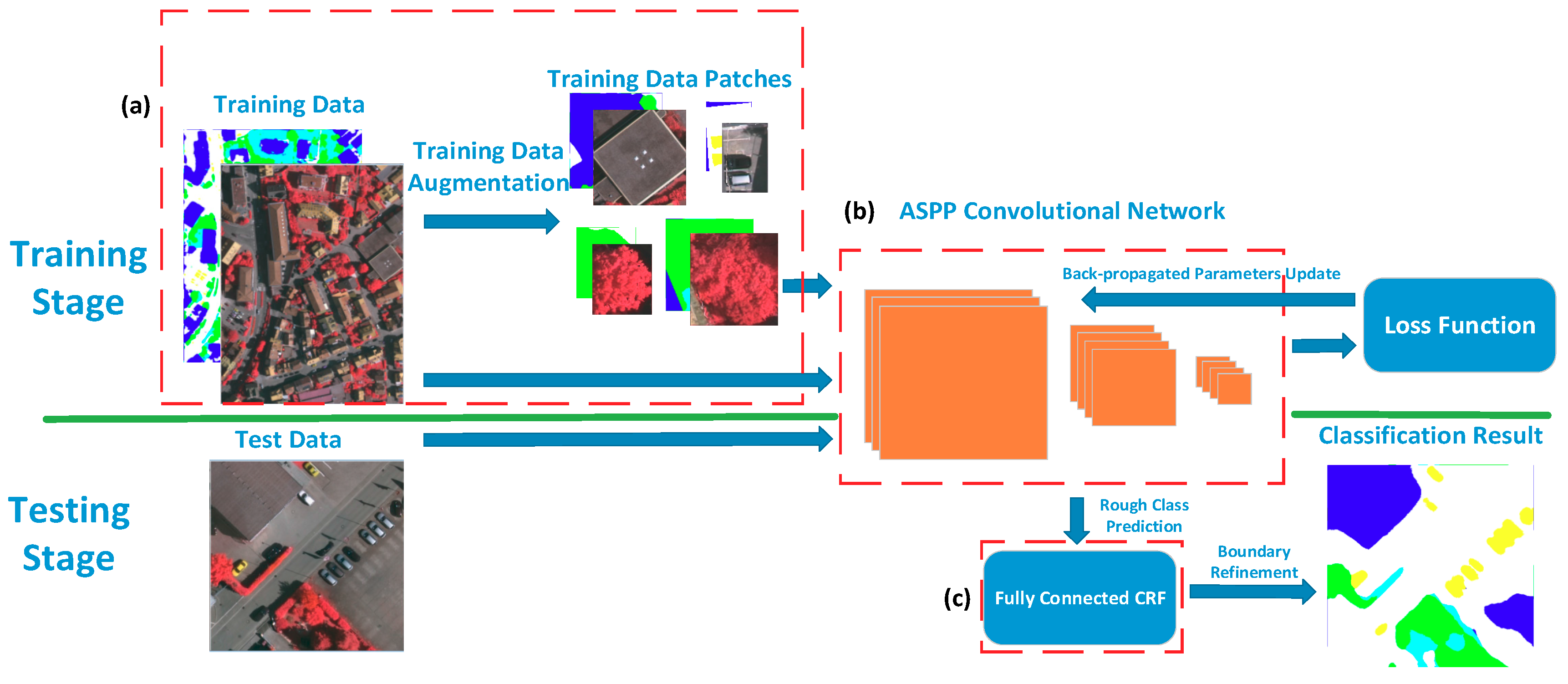
Similar to other supervised classification approaches, our proposed method generally contains two stages: the training stage and the testing stage, as illustrated in Figure 1. In the training stage, the image data and labeled data, with pixel-class correspondence, are first processed to generate training data patches that contain potential ground objects by using a pre-segmentation and selective method. Subsequently, the original training data and the augmented training data patches are both put into the ASPP convolutional network as training samples. The error between the predicted class labels and the ground truth (GT) labels is calculated and back-propagated through the network using the chain rule; subsequently, the parameters of the ASPP network are updated using the stochastic gradient descent method. The training iteration is terminated when the error is less than a given threshold.

In the testing stage, the test image data is put into the trained ASPP network model to generate a rough class prediction. The latter, together with the input image, is subsequently input into the fully connected CRFs’ post-processing module to generate the final refined classification result.

In the following sections, we will present training data augmentation processing using pre-segmentation and selective search method and explain the use of an ASPP neural network for pixel-wise image classification, post-processing using fully connected CRFs to generate the final refined classification result, and the application of such results to high-resolution remote sensing imagery.

3.1. Training Data Augmentation

As a CNN requires a large corpus of training data to achieve a satisfactory accuracy, if there are insufficient quality training data, the trained network will be overfit, i.e., become highly biased to data to which it was trained. The result of overfitting is that the network will not be able to generalize the learned model to any other samples [49]. A number of techniques have been developed to avoid overfitting, primarily including data augmentation, weight decay and dropout [50]. Weight decay and dropout are embedded in the design of the network. If the number of ground truth images is limited, it is better to perform data augmentation to improve performance. This procedure consists of creating new synthetic training examples from those already available. For image data, augmentation is the pre-processing that augments the training set via domain-specific transformations, including random cropping and random perturbations of brightness, saturation, hue and contrast.

However, the above transformations lack relevance to the ground objects. Object proposal methods could be used to find regions that might contain significant objects in the image. There are several kinds of object proposal methods, such as the grouping proposal method, e.g., selective search [51], the window scoring proposal method, e.g., EdgeBoxes [52], and the agglomerative clustering proposal method using mixtures of non-Gaussian distributions [53]. In this paper, we use an efficient graph-based method [54] to segment the ground truth images into small components; subsequently, based on the segmented components, the selective search method is applied to generate bounding boxes of potential objects. Thus, we obtain more valuable trained data with unsupervised methods than with simple augmentation.

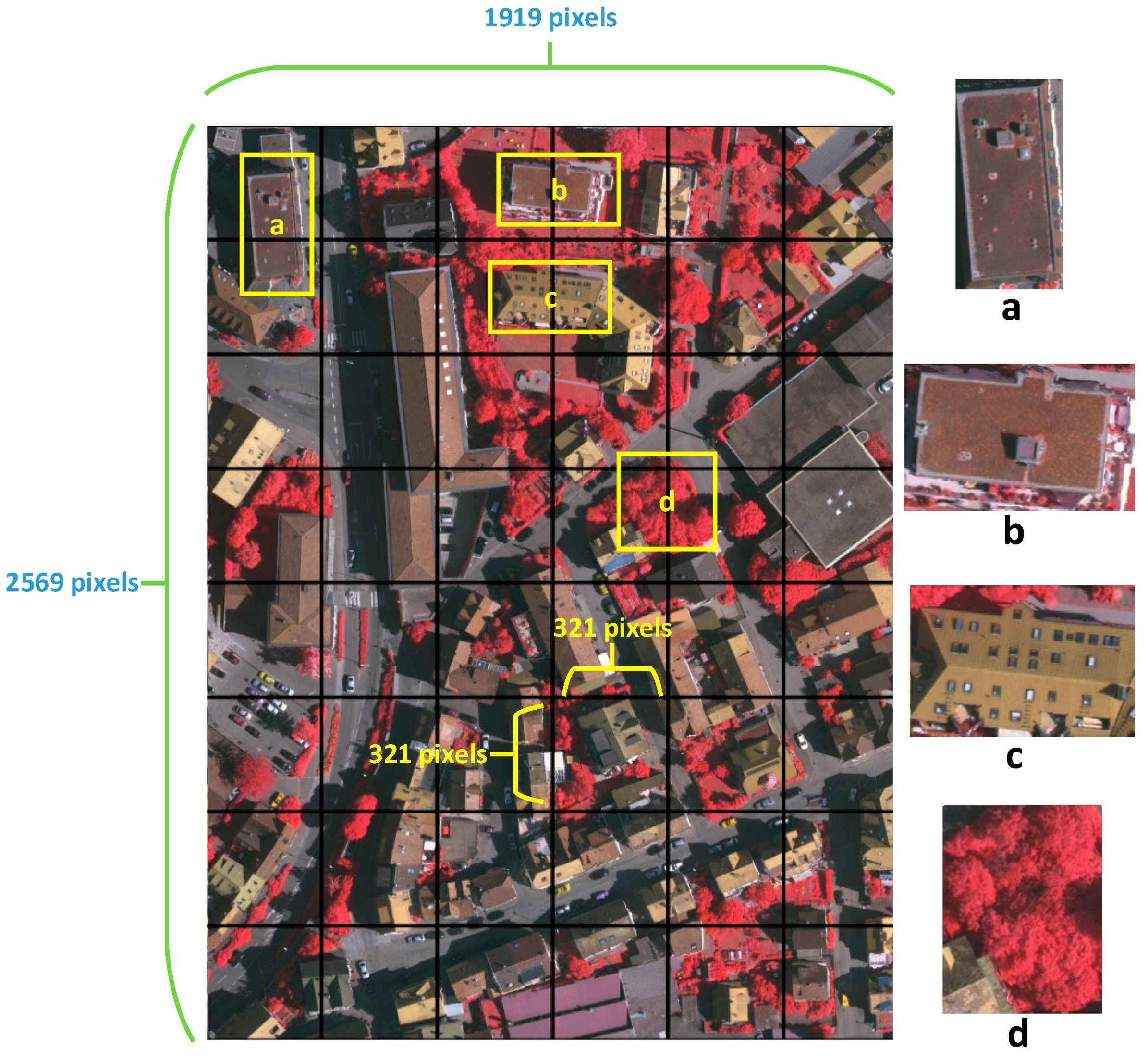
The size of high-resolution remote sensing imagery is large due to the rich information it contains that differs from natural images. Thus, it is impossible to put the entire image in a CNN in the training stage due to the network structure and limited memory. The best approach is to cut the entire image into small patches to meet the needs of the network. However, as shown in Figure 2, numerous ground objects are separated into neighbor patches, causing a loss of shape and texture features of the object. In this section, we extract potential ground objects and their labels from the ground truth data as supplements of training data.

3.1.1. Pre-Segmentation

Using the segmentation method [54], we apply a graph-based greedy decision method that could take into account the global features of an image. An important characteristic of the method is its ability to preserve detail in low-variability image regions, while ignoring detail in high-variability regions.

Let $G=\left(V,E\right)$ be an undirected graph with vertices $v_i\in V$ and edges $\left(v_i,v_j\in E\right)$. The pixels of an image could be represented by vertices of a graph. Thus, the pixels that need to be segmented constitute the set of vertices $V$. There is also a corresponding weight $w\left(\left(v_i,v_j\right)\right)$ for each edge $\left(v_i,v_j\in E\right)$ that is a non-negative measure of dissimilarity of neighboring elements $v_i$ and $v_j$. The goal of image segmentation is to find a partition of set $V$ such that each component of the partition is a connected graph $G_i=\left(V,E_i\right)$, where $E_i\subseteq E$. Based on the guideline that the weights measure the amount of dissimilarity of two vertices, we can infer that the edges between vertices of the same component will have lower weights than edges between vertices belonging to different components.

The internal difference of a component $C\subseteq V$ is defined to be the largest weight in the minimum spanning tree of the component, i.e.,

$$Int\left(C\right)=\underset{e\in MST\left(C,E\right)}{\max }w\left(e\right)$$

(1)

where $MST\left(C,E\right)$ denotes the minimum spanning tree of the sub-graph $G=\left(C,E\right)$. A minimum spanning tree is the sub-graph that connects all vertices $C$ and has the least sum total of weights. The difference between two components is defined to be the minimum edge weight connecting the two components, i.e.,

$$Dif\left(C_1,C_2\right)=\underset{v_i\in C_1,v_j\in C_2,\left(v_i,v_j\right)\in E}{\min }w\left(\left(v_i,v_j\right)\right)$$

(2)

If there is no edge connecting $C_i$ and $C_j$, then $Dif\left(C_i,C_j\right)=\infty$.

$Dif\left(C_i,C_j\right)$ is large relative to the internal difference within at least one of the components. A threshold function is used to control the degree to which the difference between components must be larger than the minimum internal difference. The pairwise comparison is defined as

$$D\left(C_1,C_2\right)=\{\begin{array}{ll}true& ifDif\left(C_1,C_2\right)>MInt\left(C_1,C_2\right)\\ false& otherwise\end{array}$$

(3)

where the minimum internal difference, $MInt\left(C_1,C_2\right)$, is defined as

$$Mint\left(C_1,C_2\right)=\min \left(Int\left(C_1\right)+\tau \left(C_1\right),Int\left(C_2\right)+\tau \left(C_2\right)\right)$$

(4)

The threshold function is defined as

$$\tau \left(C\right)=k/\left|C\right|$$

(5)

where $\left|C\right|$ denotes the size of $C$. $k$ is a constant parameter that is set manually in the experiments, with a larger $k$ causing a preference for larger components. The threshold function above implies that for small components, we require a strong evidence for a boundary.

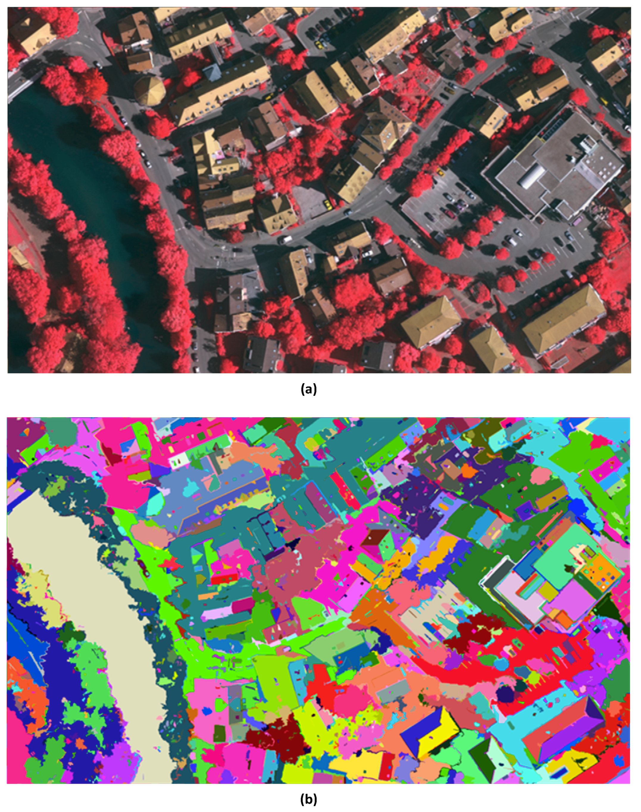
After pre-segmentation, the original image is segmented into many small regions, also known as superpixels. The original image and the image resulting from segmentation are shown in Figure 3. We can observe a coarse segmentation into small segmented regions of different colors. In the next step, the small segmented regions are input to the selective search method to generate image patches that might contain potential ground objects, such as buildings, trees and cars.

3.1.2. Selective Search

Selective search is an efficient unsupervised objectness proposal method that combines the strengths of both exhaustive search and segmentation. In this step, small segmented regions generated by the preceding pre-segmentation step are merged into larger regions by different measures of similarity. To determine whether two image regions belong to the same object, various measures of similarity are considered, including, but not limited to, color, texture and size. As a kind of structural similarity, MSSIM [55] is a popular similarity index that can also be added to the measures.

$s_{colour}\left(r_i,r_j\right)$ measures color similarity. The color histograms are normalized using the L1 norm. Similarity is measured by the histogram intersection:

$$s_{colour}\left(r_i,r_j\right)={\displaystyle \sum }_{k=1}^n\min \left(c_i^k,c_j^k\right)$$

(6)

$s_{texture}\left(r_i,r_j\right)$ measures texture similarity using SIFT-like measurements. Gaussian derivatives in eight orientations are calculated for each color channel, where $\sigma =1$. For each orientation of each color channel, a histogram using a bin size of 10 is extracted. Thus, a texture histogram $T_i=\left\{T_{i1},\dots ,T_{in}\right\}$ for each region $r_i$ with dimensionality n = 240 could be constructed if three color channels are considered. Similarity is measured by using the histogram intersection:

$$s_{texture}\left(r_i,r_j\right)={\displaystyle \sum }_{k=1}^n\min \left(t_i^k,t_j^k\right)$$

(7)

$s_{size}\left(r_i,r_j\right)$ encourages small regions to merge early and is defined as the fraction of the image that $r_i$ and $r_j$ jointly occupy, where size(im) denotes the size of the image in pixels:

$$s_{size}\left(r_i,r_j\right)=1-\frac{size\left(r_i\right)+size\left(r_j\right)}{size\left(im\right)}$$

(8)

$s_{fill}\left(r_i,r_j\right)$ measures how well regions $r_i$ and $r_j$ fit into each other. $B{B}_{ij}$ is defined to be the tight bounding box around $r_i$ and $r_j$. $s_{fill}\left(r_i,r_j\right)$ is the fraction of the image contained in $B{B}_{ij}$ that is not covered by regions $r_i$ and $r_j$:

$$s_{fill}\left(r_i,r_j\right)=1-\frac{size\left(B{B}_{ij}\right)-size\left(r_i\right)-size\left(r_j\right)}{size\left(im\right)}$$

(9)

The final similarity measure combines the above four strategies:

$$s\left(r_i,r_j\right)=a_1{s}_{colour}\left(r_i,r_j\right)+a_2{s}_{texture}\left(r_i,r_j\right)+a_3{s}_{size}\left(r_i,r_j\right)+a_4{s}_{fill}\left(r_i,r_j\right)$$

(10)

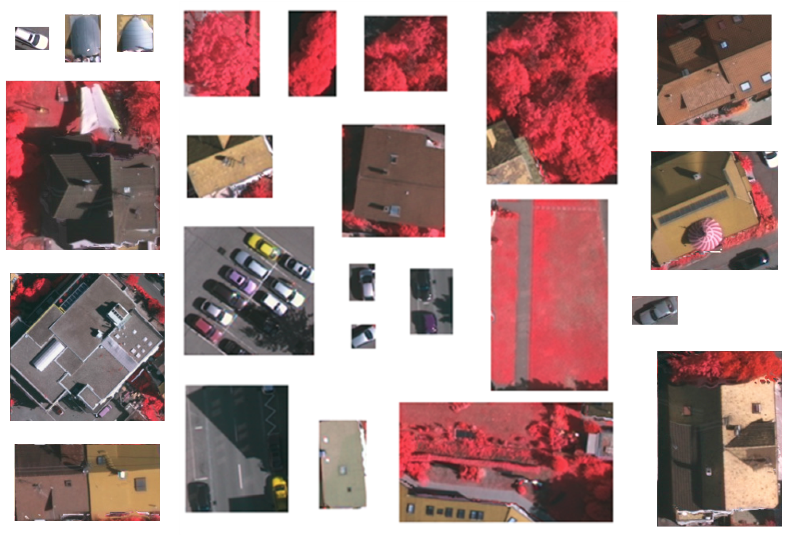
All regions are combined and sorted by the order in which they were generated, starting with the region from every iteration of merging that was generated last. This order reflects the likelihood of regions to contain an object. Duplicate bounding boxes are removed after sorting. Figure 4 shows the extracted bounding boxes of potential ground objects that could be added to the training dataset.

After applying the selective search method, images of bounding boxes of potential ground objects are generated along with the respective label data. In the next step, the images of bounding boxes and the respective labeled images together with the original images and labels are put into the subsequent CNN-based classification step for model training.

3.2. Pixel-Wise Classification Using CNN

In this section, we present our novel CNN architecture for pixel-wise classification of remote sensing imagery. First, the section details the characteristics of FCN, followed by the advantages of atrous convolution and the ASPP network architecture that applies the atrous convolution. The ASPP network uses the augmented training data generated by the preceding section on model training.

3.2.1. Fully Convolutional Network

The traditional CNN-based segmentation approaches typically separate a large image into small patches; the semantic labeling process can be regarded as classifying the central pixel of each image patch. To label the entire image, the prediction must thus be performed on many overlapping image patches, requiring a large amount of redundant calculations and memory. The patch size also limits the receptive field of the network and cannot extract multi-scale features of the image. The FCN is one of the CNN variants that has been proven to be state-of-the-art for semantic segmentation in natural images. An FCN is characterized by three primary features.

The first typical feature of an FCN is that the fully connected layers are replaced by fully convolutional layers. In a CNN, the network is usually finished by a fully connected layer that converts 2D feature maps to a 1D vector, with the probability of each class subsequently computed by methods such as softmax. The fully connected layers have fixed-length dimensions and discard spatial information. An FCN naturally operates on an image of any size, producing an output of corresponding spatial dimensions.

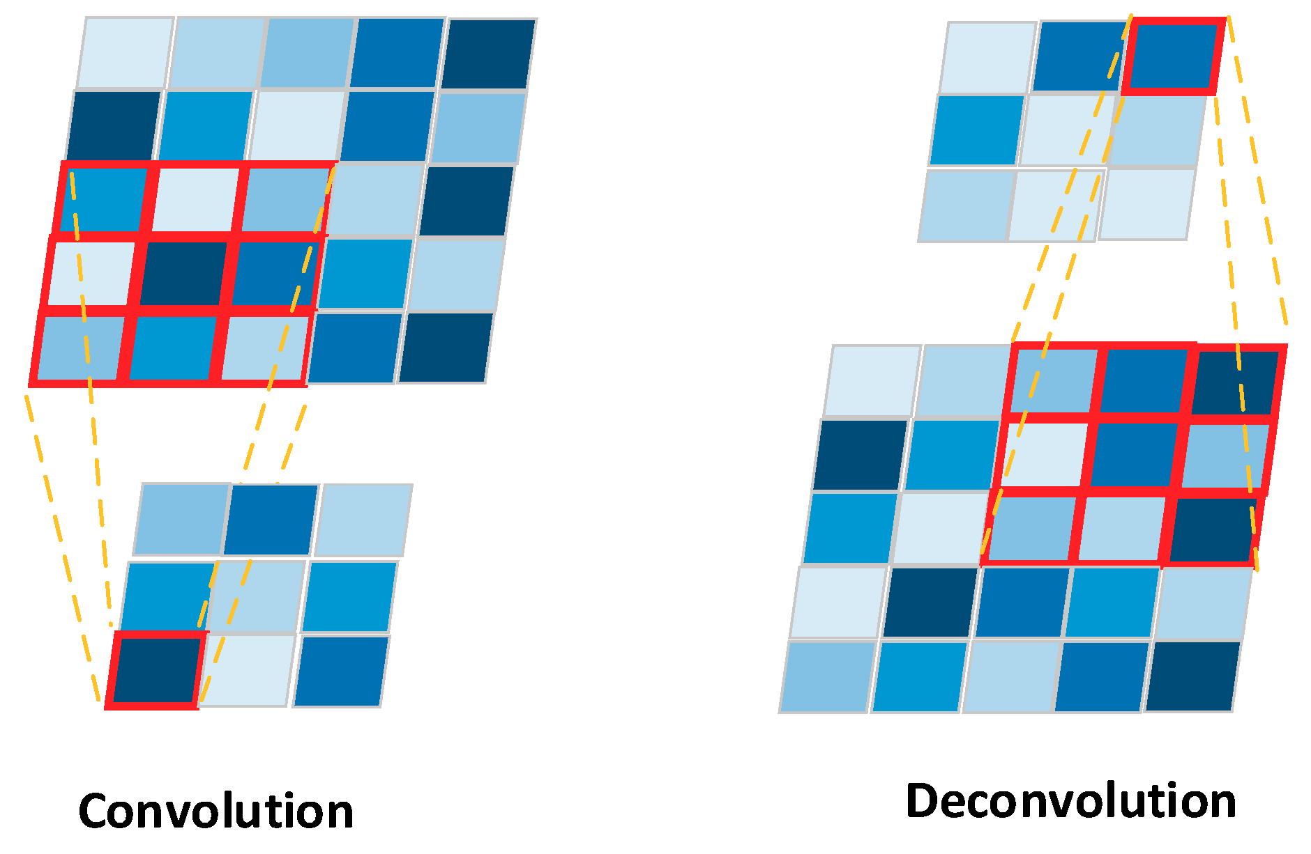
Deconvolution is the second feature of FCN. A deconvolution, also called Transposed Convolution or Fractional Strided Convolution, performs a regular convolution while reverting its spatial transformation, as shown in Figure 5. For image segmentation, a deconvolution layer is put on top of a regular CNN. It is used for upsampling the output of a CNN to obtain the same size as the input image. The down-sampled feature maps from CNN are upsampled through the deconvolution layer, generating features that can be used to predict the class label of each pixel. Such predictions are compared to ground truth segmentation labels; a loss function is defined that guides the network towards correct predictions by updating parameters in backward propagation, as usual.

The third feature of an FCN is the skip layer architecture. For example, in the VGG16 network, the FC-8s is improved from FCN-16s skip net and FCN-32s coarse net. The skip layer is used to combine dense predictions at shallow layers, and coarse predictions at deep layers, which can improve segmentation details. More specifically, FCN-16s is a skip net that combines twice upsampled predictions computed on the last layer at stride 32 with predictions from Pool4 at stride 16. In the same way, FCN-8s is implemented by fusing predictions of the shallower layer Pool3 with twice-upsampled the sum of two predictions derived from Pool4 and the last layer. The stride 8 predictions are subsequently upsampled back to the image. As a result, FCN-8s produces more detailed segmentations than FCN-16 and FCN-32s.

3.2.2. Atrous Convolution

The use of FCN for semantic segmentation has been shown to be simple and successful. However, the repeated combination of pooling and striding operations at consecutive layers of such networks reduces the spatial resolution of the resulting feature maps. Although deconvolution layers could be used, the result is also coarse. Yu [29] showed that atrous convolution enlarges the field-of-view of filters without the loss of resolution or coverage.

Atrous convolution is also called dilated convolution. The primary idea of atrous convolution is to insert a zero-value hole between pixels in convolutional kernels to increase the image resolution that could enable dense feature extraction in a deep CNN. In the 1D signal convolution case, given the input signal $x\left[i\right]$ with a filter $w\left[k\right]$ of length $k$, the output of atrous convolution $y\left[i\right]$ is calculated as:

$$y[i]={\displaystyle \sum }_{k=1}^{K}x[i+r·k]w[k]$$

(11)

The rate parameter $r$ corresponds to the stride with which the input signal is sampled, with the standard convolution being the special case of rate r = 1.

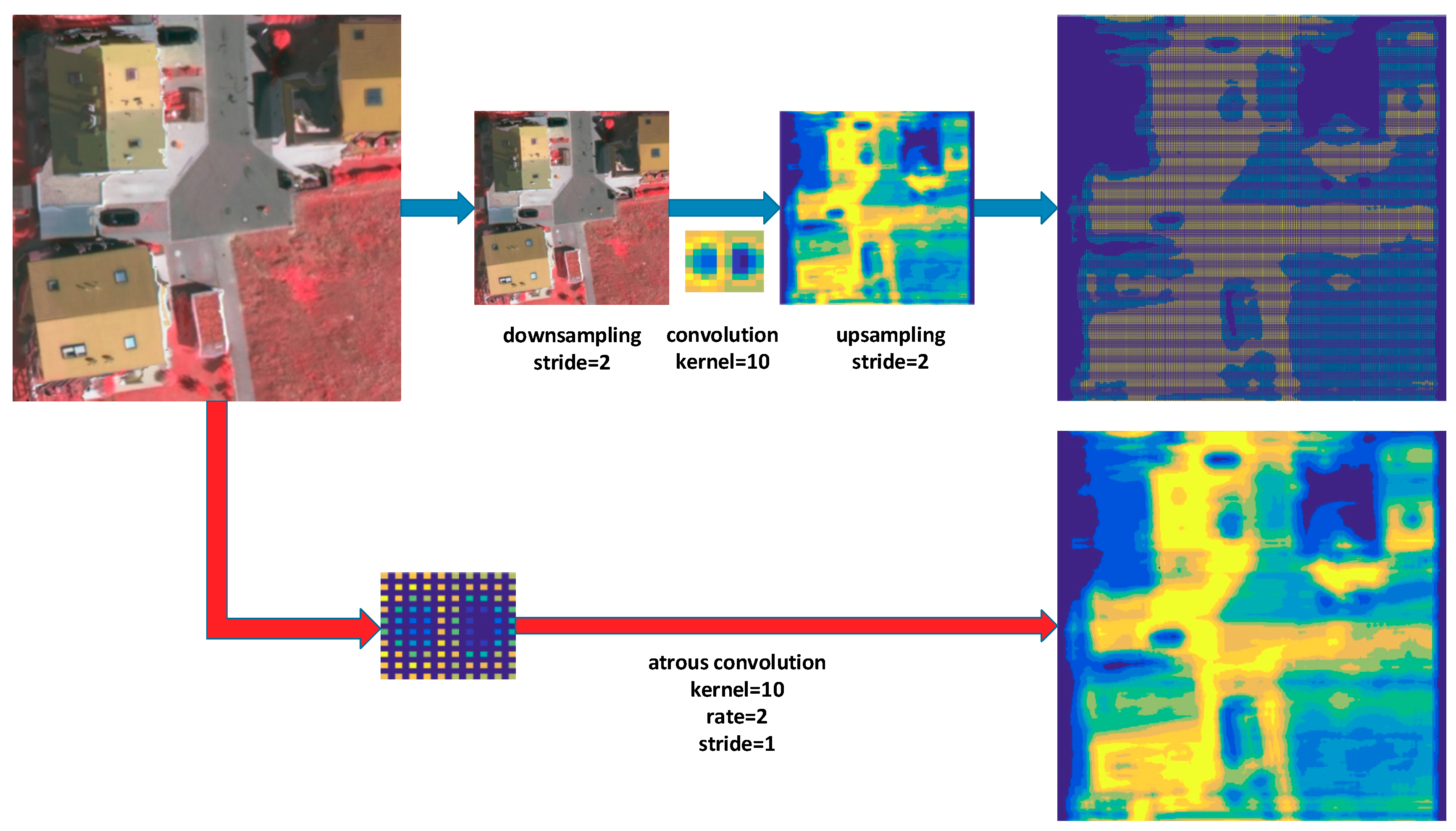
We explain the atrous convolution’s operation through an example in Figure 6. First, we downsample an image, reducing the resolution by a factor of 2, and subsequently perform a convolution with a 10 × 10 kernel. Then, an upsampling operation is performed to generate the feature map of the same size as the original image. Compared to the original image coordinates, we have obtained responses at only 1/4 of image positions. Instead, if we convolve the full-resolution image with a filter ‘with holes’ of size 19 × 19, we can obtain a feature map at all image positions. Due to atrous convolution, the receptive field of the network is larger, while the feature map is denser. The results allow us to control the spatial resolution of neural network feature maps easily and explicitly.

3.2.3. Network Architecture

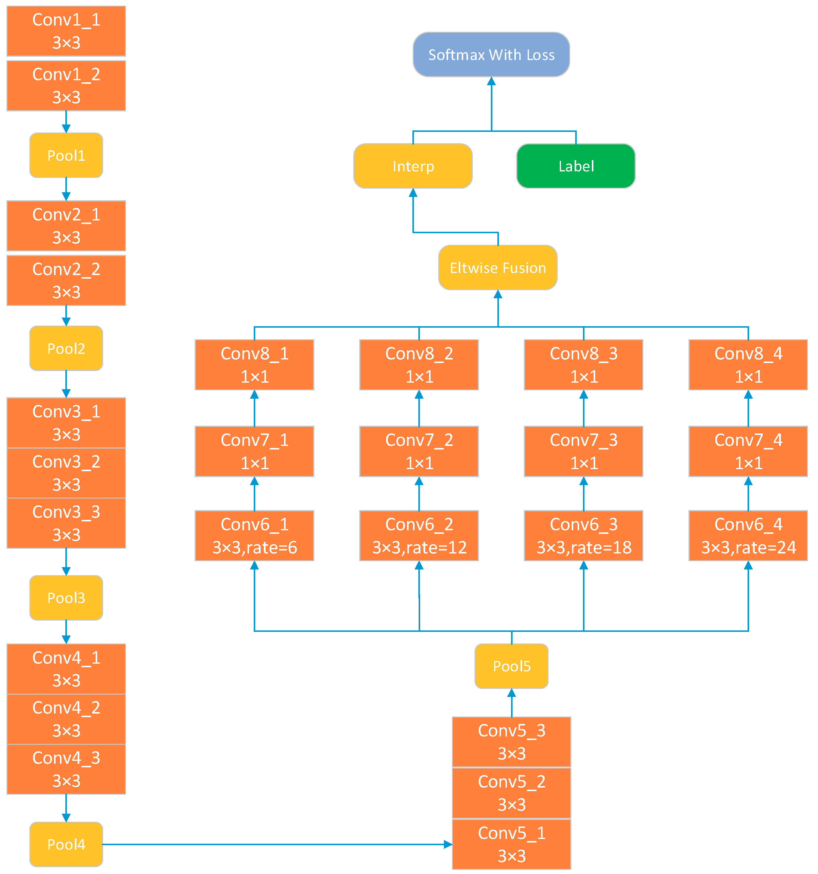
We used an ASPP network with the architecture shown in Figure 7. It is derived from a VGG-16 [28] network and has the same architecture until the Pool5 operation. ASPP for VGG-16 replaces layers fc6, fc7 and fc8 with parallel fully convolutional layers conv6, conv7 and conv8. The conv6 branch layers use 3 × 3 kernels, yet apply different atrous rates to capture objects of different sizes. The conv7 and conv8 layers use 1 × 1 kernels. After all convolution operations, the branch layers are combined by element-wise fusion. Subsequently, a simple bilinear interpolation is performed to enlarge the feature maps to the original image size. Finally, the softmax loss layer is created on top of the last layer that computes the multinomial logistic loss of the softmax of its inputs.

3.3. Fully Connected CRFs

FCN-based models and atrous convolution have proven to be the most successful methods of semantic segmentation. However, the increased invariance and the large receptive fields can only predict the rough positions of objects but cannot delineate their borders. Traditionally, conditional random fields (CRFs) could be used as a post-processing tool to refine segmentation results. Thus, the fully connected CRFs [56] model is integrated with the flow.

The model employs the energy function:

$$E(x){\displaystyle \sum }_i{\theta }_i(x_i)+{\displaystyle \sum }_{ij}{\theta }_{ij}(x_i,x_j)$$

(12)

where $x$ is the label assignment for pixels. ${\theta }_i\left(x_i\right)=-\log P\left(x_i\right)$ represents the unary potential, where $P\left(x_i\right)$ is the label assignment probability at pixel $i$ predicted by a CNN. ${\theta }_{ij}\left(x_i,x_j\right)$ is the pairwise potential represented by a fully connected graph, connecting all pairs of the predicted image pixels $i$ and $j$. The pairwise potential is defined as follows:

$${\theta }_{ij}(x_i,x_j)=\mu (x_i,x_j)[w_1\exp (-\frac{\Vert p_i-p_j{\Vert }^2}{2{\theta }_{\alpha }^2}-\frac{\Vert I_i-I_j{\Vert }^2}{2{\theta }_{\beta }^2})+w_1\exp (-\frac{\Vert p_i-p_j{\Vert }^2}{2{\sigma }_{\gamma }^2})]$$

(13)

where $\mu \left(x_i,x_j\right)$ = 1 if $x_i\ne x_j$ and zero otherwise, i.e., as in the Potts model, only nodes with distinct labels are penalized. The remaining expression uses two Gaussian kernels in different feature spaces; the first, ‘bilateral’, kernel depends on both pixel positions (denoted as p) and RGB color (denoted as I), while the second kernel only depends on pixel positions. The hyper parameters ${\sigma }_{\alpha }$, ${\sigma }_{\beta }$ and ${\sigma }_{\gamma }$ control the scale of Gaussian kernels. The first kernel forces pixels with similar colors and positions to have similar labels, while the second kernel only considers the spatial proximity to enforce smoothness.

In CRF post-processing, the coarse class labels predicted by the FCN are input as the unary potential. Along with the original image that provides the pairwise potential with position and color information, the class labels are adjusted and refined under the position-color constraints.

4. Results

We performed extensive experiments to assess the effectiveness of our proposed method. We test the method on a benchmark of aerial image labeling, the Vaihingen dataset, provided by Commission III of the International Society for Photogrammetry and Remote Sensing (ISPRS) [57]. In this section, we describe the datasets and the training settings in the experiment and present numerical and visual results. We evaluate the benefits of each component of our proposed method and compare our results to those of the base FCN, FCN-8s, MLP and ASPP networks. Our experiment was based on the Caffe [58] platform and performed on a computer running the Windows 7 operating system and equipped with an NVIDIA GeForce GTX1080 Ti [59] graphics card with 11 GB of memory.

4.1. Datasets

The Vaihingen dataset is composed of 33 image tiles, of which 16 are fully annotated with class labels. The 16 image tiles are labeled into the following six classes: impervious surface, building, low vegetation, tree, car, and background. The spatial resolution is 9 cm. Near-infrared (NIR), red (R) and green (G) bands are provided. We select 4 images for testing (IDs: 30, 32, 34, and 37) and use the remaining 12 images for training.

4.2. Training

The network is trained by stochastic gradient descent. To fit the network architecture, we cut the original images into small patches of various sizes (321 × 321, 353 × 353, 385 × 385, 417 × 417, 449 × 449, 481 × 481, and 513 × 513) supplemented with the augmentation patches by the selective search method, performing random flips (vertically, horizontally, or both) and mirroring. In every iteration, a group of patches is fed to the network for backpropagation; the size of patches is also called the batch size. In all cases, a momentum of 0.9 and an L2 penalty on the network’s weight decay of 0.0005 are used. The interpolation layer uses a factor of 8 to resize the feature maps to the original image. Weights are initialized following [16], and as we use batch normalization layers before ReLUs, there is no need to normalize the input channels. Training ends after 20,000 iterations in the first dataset and 20,000 in the second, when the error stabilizes on the validation set. To train the base FCN, FCN-8s and MLP networks, we initialize the weights with the pretrained base FCN and jointly retrain the entire architecture. We start this second training phase with a learning rate of 0.01 and stop it after 30,000 and 65,000 iterations for the Vaihingen dataset.

4.3. Results and Comparison

We evaluate the performance of various methods based on three criteria: per-class accuracy, the overall accuracy and the average F1-score. The accuracy is defined as the number of true positives ($TP$) divided by the sum of the number of true positives and the number of false positives ($FP$):

$$accuracy=\frac{TP}{TP+FP}$$

(14)

Recall is defined as the number of true positives ($TP$), divided by the sum of the number of true positives and the number of false negatives ($FN$):

$$recall=\frac{TP}{TP+FN}$$

(15)

In addition, the F1-score is defined as:

$$F1-score=2\times \frac{accuracy\times recall}{\left(accuracy+recall\right)}$$

(16)

4.3.1. Numerical and Visual Results Comparison

Due to limited GPU memory, the test images are tiled into 513 × 513 patches in the testing stage. Subsequently, the patches are processed by the trained model to obtain the coarse results. Finally, the original test image patches and the coarse results are both put into Fully Connected CRFs, and the results are generated.

Table 2. Results of experiments on the Vaihingen dataset.

Approach	Impervious Surface	Building	Low Vegetation	Tree	Car	Average F1-Score	Average Recall	Overall Accuracy
Basic FCN	81.40	86.83	76.51	81.94	68.09	77.72	76.79	81.57
FCN-8s	82.28	88.12	76.66	81.93	70.06	79.16	77.39	82.24
MLP	84.01	88.95	78.82	82.72	70.95	82.28	80.43	83.65
ASPP	89.39	91.73	79.34	84.08	71.51	85.00	85.05	86.48
Ours	91.03	92.94	80.13	87.25	74.12	86.84	87.06	88.13

reports the experimental results obtained using the Vaihingen dataset. The building and impervious surface classes are identified with a higher accuracy than others. The accuracy of the car class is the lowest due to cars containing fewer pixels, easily leading to information loss in the pooling operation. Confusion matrices are also provided in

Table 3. Confusion matrix for the Vaihingen dataset.

	Reference → Predictions ↓	Impervious Surface	Building	Low Vegetation	Tree	Car
	Impervious Surface	81.4	5.12	4.57	4.64	22.65
	Building	6.89	86.83	3.34	2.51	3.58
Basic FCN	Low Vegetation	6.01	3.74	76.51	10.68	2.92
	Tree	4.57	3.78	14.6	81.94	2.76
	Car	1.13	0.52	0.97	0.23	68.09
	Impervious Surface	82.28	6.21	6.03	2.88	24.29
	Building	5.61	88.12	1.91	1.51	3.38
FCN-8s	Low Vegetation	8.31	1.95	76.66	13.32	1.51
	Tree	3.02	2.13	15.11	81.93	0.76
	Car	0.78	1.59	0.28	0.35	70.06
	Impervious Surface	84.01	6.35	5.83	3.32	23.38
	Building	4.29	88.95	1.3	1.97	3.44
MLP	Low Vegetation	7.13	2.93	78.82	11.52	1.46
	Tree	3.89	1.18	13.69	82.72	0.76
	Car	0.68	0.49	0.36	0.46	70.95
	Impervious Surface	89.39	3.57	5.91	2.49	21.12
	Building	2.99	91.73	3.84	0.81	4.61
ASPP	Low Vegetation	5.33	2.13	79.34	12.48	1.87
	Tree	1.93	2.2	10.82	84.08	0.89
	Car	0.36	0.36	0.08	0.13	71.51
	Impervious Surface	91.03	3.97	6.74	1.91	19.98
	Building	3.12	92.94	3.55	0.43	3.08
Ours	Low Vegetation	3.09	1.21	80.13	10.31	2.57
	Tree	2.34	1.8	9.41	87.25	0.24
	Car	0.42	0.08	0.17	0.09	74.12

for the experiment based on the ground truth for the Vaihingen dataset.

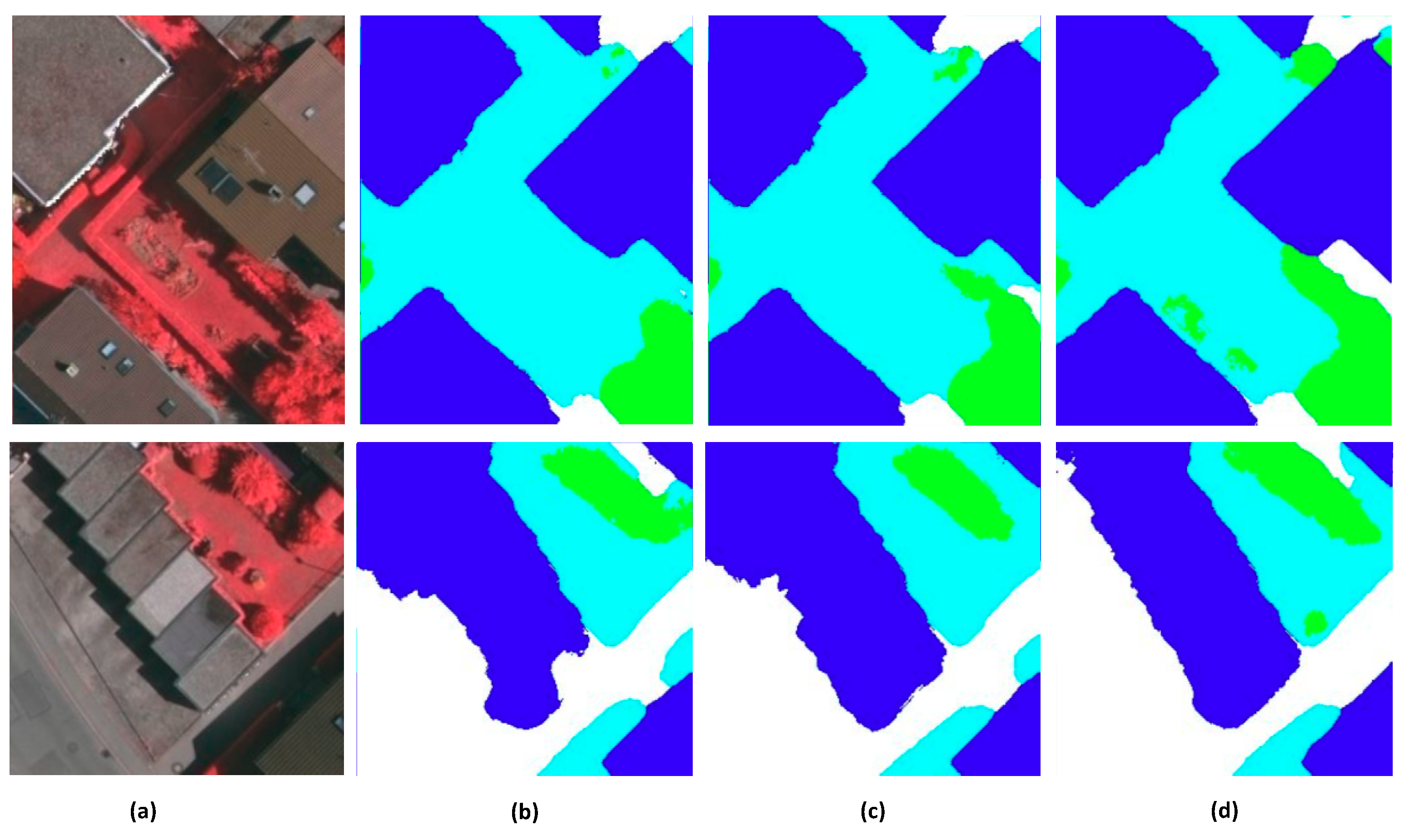
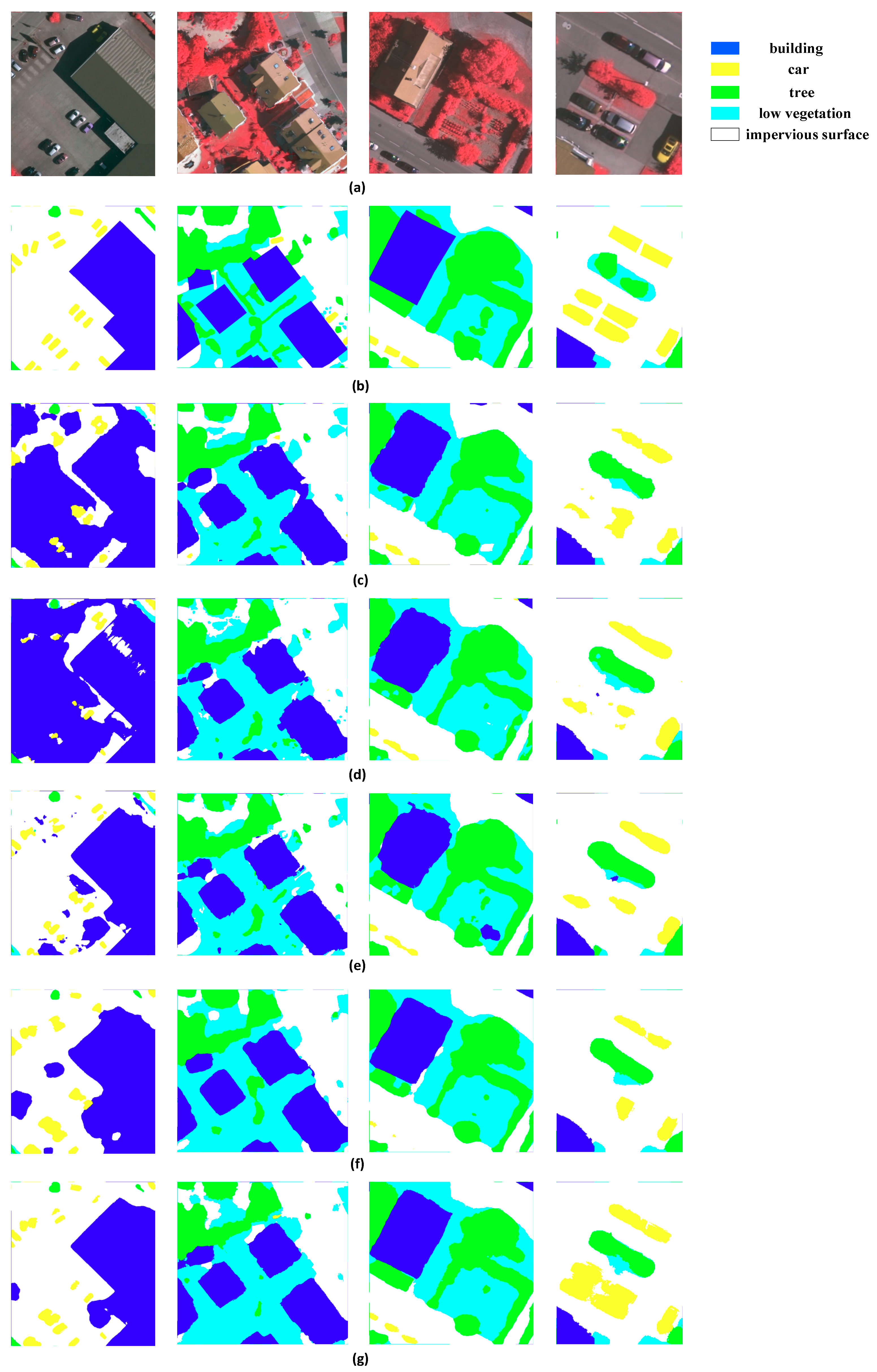
We show a visual comparison of classified images in Figure 8. The base FCN and FCN-8s tend to output blob-like objects, while other methods provide sharper results. The outputs of base FCN and FCN-8s are not fine enough, resulting in a loss of valuable detailed information. Certain impervious surface areas are also mistaken for buildings. The MLP method combines feature maps of different convolutional layers, with the results looking better than those of base FCN and FCN-8s. We observe that MLP tends to identify boundaries more accurately at a fine level. Unlike MLP, ASPP exploits multi-scale features by employing multiple parallel filters with different rates, and subsequently refining the output by fully connected CRFs. The results of ASPP for buildings are comparatively regular. Our method is based on ASPP and the training data augmentation, with Figure 8 showing that our method’s results are closer than those of other methods to the ground truth data.

4.3.2. Computational Complexity Comparison

For supervised networks such as CNNs, deeper layers can learn more complex distributions [60], yet may result in more parameters to learn and a need for greater computing resources. Thus, computational complexity becomes a vital factor to consider. The total time complexity [61] of all convolutional layers is

$$O({\displaystyle \sum }_{l=1}^d{n}_{l-1}\cdot s_l^2\cdot n_l\cdot m_l^2)$$

(17)

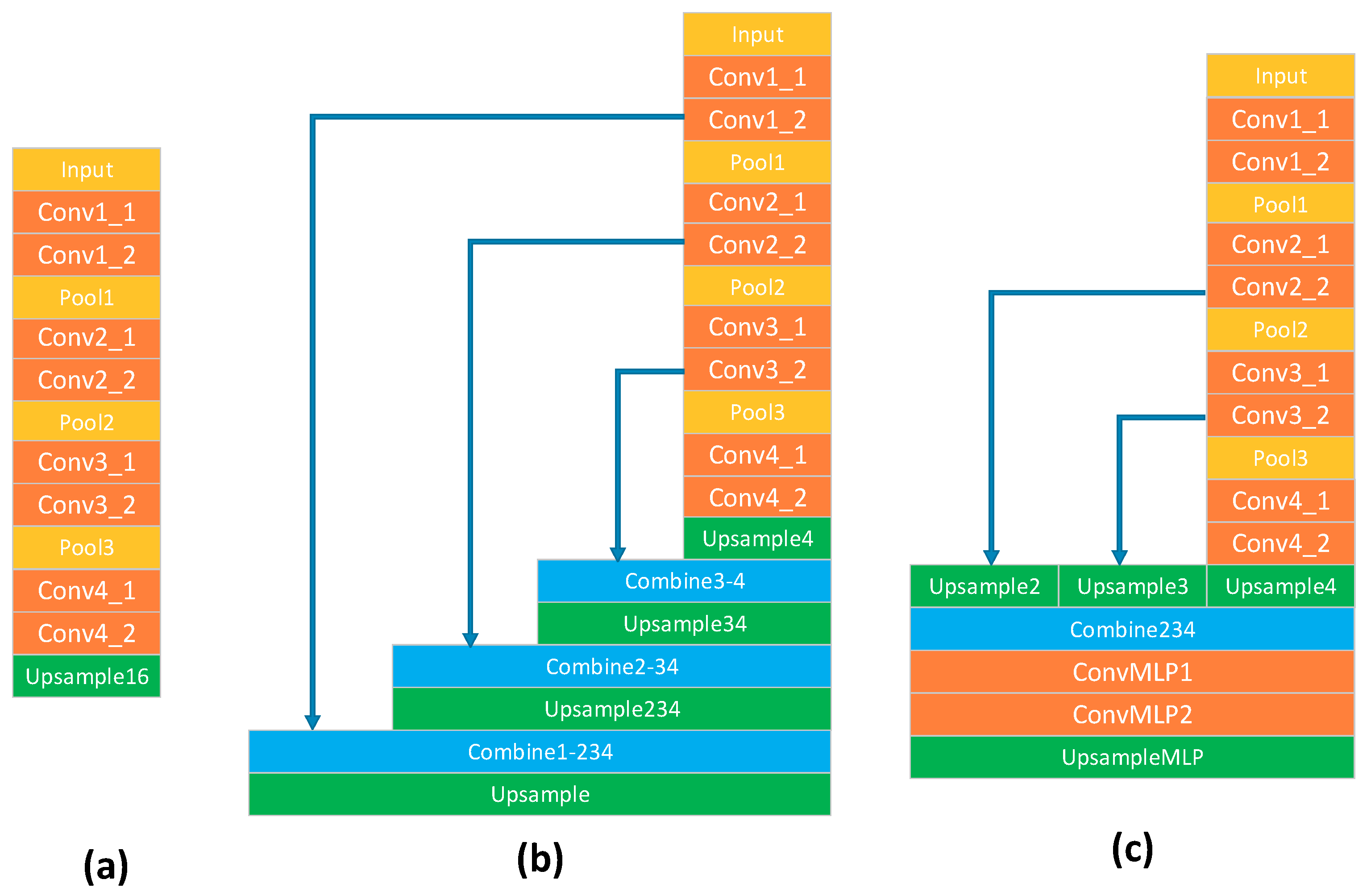
where $l$ represents the index of a convolutional layer, and $d$ represents the number of convolutional layers. $n_l$ represents the number of filters in the l-th layer. $n_{l-1}$ is also known as the number of input channels of the l-th layer. $s_l$ is the spatial size of the filter. $m_l$ is the spatial size of the output feature map. The above time complexity applies to both training and testing times. The time cost of fully connected layers and pooling layers is not included in the above formulation. Such layers often take 5–10% of computation time. We only consider the trade-offs among the convolutional layers. We show the network architectures of Base FCN, FCN-8s and MLP in Figure 9, and the parameters of convolutional layers in

Table 4. Convolutional Layer Parameters of the Base FCN and FCN-8s.

Layer ($\mathit{l}$)	Filter Size (${\mathit{s}}_{\mathit{l}}$)	Number of Filters (${\mathit{n}}_{\mathit{l}}$)	Number of Input Channels (${\mathit{n}}_{\mathit{l}-1}$)	Spatial Size of Output Feature Map (${\mathit{m}}_{\mathit{l}}^2$)	Stride	Padding
Input			3	$H_0\times W_0$
Conv-1_1	5	32	3	$H_0/2\times W_0/2$	2	2
Conv-1_2	3	32	32	$H_0/2\times W_0/2$	1	1
Pool-1	2	32	32	$H_0/4\times W_0/4$	2
Conv-2_1	3	64	32	$H_0/4\times W_0/4$	1	1
Conv-2_2	3	64	64	$H_0/4\times W_0/4$	1	1
Pool-2	2	64	64	$H_0/8\times W_0/8$	2
Conv-3_1	3	96	64	$H_0/8\times W_0/8$	1	1
Conv-3_2	3	96	96	$H_0/8\times W_0/8$	1	1
Pool-3	2	96	96	$H_0/16\times W_0/16$	2
Conv-4_1	3	128	96	$H_0/16\times W_0/16$	1	1
Conv-4_2	3	128	128	$H_0/16\times W_0/16$	1	1
Upsample16	32	5	128	$H_0\times W_0$	16	8

,

Table 5. Convolutional Layer Parameters of MLP.

Layer ($\mathit{l}$)	Filter Size (${\mathit{s}}_{\mathit{l}}$)	Number of Filters (${\mathit{n}}_{\mathit{l}}$)	Number of Input Channels (${\mathit{n}}_{\mathit{l}-1}$)	Spatial Size of Output Feature Map (${\mathit{m}}_{\mathit{l}}^2$)	Stride	Padding
Input			3	$H_0\times W_0$
Conv-1_1	5	64	3	$H_0/2\times W_0/2$	1	1
Conv-1_2	3	64	64	$H_0/2\times W_0/2$	1	1
Pool-1	2	64	64	$H_0/4\times W_0/4$	2
Conv-2_1	3	96	64	$H_0/4\times W_0/4$	1	1
Conv-2_2	3	96	96	$H_0/4\times W_0/4$	1	1
Pool-2	2	96	96	$H_0/8\times W_0/8$	2
Conv-3_1	3	128	96	$H_0/8\times W_0/8$	1	1
Conv-3_2	3	128	128	$H_0/8\times W_0/8$	1	1
Pool-3	2	128	128	$H_0/16\times W_0/16$	2
Conv-4_1	3	160	128	$H_0/16\times W_0/16$	1	1
Conv-4_2	3	160	160	$H_0/16\times W_0/16$	1	1
Upsample	8	128	160	$H_0/2\times W_0/2$	1
ConvMLP1	1	256	128	$H_0/2\times W_0/2$	1
ConvMLP2	1	5	256	$H_0/2\times W_0/2$	1
UpsampleMLP	4	5	5	$H_0\times W_0$	2

and

Table 6. Convolutional Layer Parameters of ASPP.

Layer ($\mathit{l}$)	Filter Size (${\mathit{s}}_{\mathit{l}}$)	Number of Filters (${\mathit{n}}_{\mathit{l}}$)		Number of Input Channels (${\mathit{n}}_{\mathit{l}-1}$)	Spatial Size of Output Feature Map (${\mathit{m}}_{\mathit{l}}$)	Stride	Padding
Input				3	$H_0\times W_0$
Conv-1_1	3		64	3	$H_0\times W_0$	1	1
Conv-1_2	3		64	64	$H_0\times W_0$	1	1
Pool-1	3		64	64	$H_0/2\times W_0/2$	2
Conv-2_1	3		128	64	$H_0/2\times W_0/2$	1	1
Conv-2_2	3		128	128	$H_0/2\times W_0/2$	1	1
Pool-2	3		128	128	$H_0/4\times W_0/4$	2
Conv-3_1	3		256	128	$H_0/4\times W_0/4$	1	1
Conv-3_2	3		256	256	$H_0/4\times W_0/4$	1	1
Conv-3_3	3		256	256	$H_0/4\times W_0/4$	1	1
Pool-3	3		256	256	$H_0/8\times W_0/8$	2
Conv-4_1	3		512	256	$H_0/8\times W_0/8$	1	1
Conv-4_2	3		512	512	$H_0/8\times W_0/8$	1	1
Conv-4_3	3		512	512	$H_0/8\times W_0/8$	1	1
Pool-4	3		512	512	$H_0/8\times W_0/8$	1
Conv-5_1	3		512	512	$H_0/8\times W_0/8$	1	2
Conv-5_2	3		512	512	$H_0/8\times W_0/8$	1	2
Conv-5_1	3		512	512	$H_0/8\times W_0/8$	1	2
Pool-5	3		512	512	$H_0/8\times W_0/8$	1
Conv-6_1 Conv-6_2 Conv-6_3 Conv-6_4	3		1024	512	$H_0/8\times W_0/8$	1	6 12 18 24
Conv-7_1 Conv-7_2 Conv-7_3 Conv-7_4	1		1024	1024	$H_0/8\times W_0/8$	1
Conv-8_1 Conv-8_2 Conv-8_3 Conv-8_4	1		1024	1024	$H_0/8\times W_0/8$	1
Upsample	1		5	1024	$H_0\times W_0$	1

. The base FCN and FCN-8s share the same convolutional layer parameters, shown in Table 4. According to the parameters of convolutional layers, we can estimate the computation time of both training and testing of each network architecture as follows:

$$tim{e}_{BaseFCN}\approx {10}^{24}\times H_0^8\times W_0^8$$

(18)

$$tim{e}_{FCN-8s}\approx {10}^{24}\times H_0^8\times W_0^8$$

(19)

$$tim{e}_{MLP}\approx {10}^{33}\times H_0^{10}\times W_0^{10}$$

(20)

$$tim{e}_{ASPP}\approx {10}^{70}\times H_0^{16}\times W_0^{16}$$

(21)

where $H_0$ represents the height of an input image and $W_0$ represents its width.

According to our estimates of computation times, the Base FCN and FCN-8s networks take almost the same time, because they have the same convolutional layers. The MLP network takes longer due to additional convolutional layers MLP1 and MLP2. The network architecture of ASPP is much deeper than those of the three abovementioned networks. In addition, as it uses atrous convolution, the computation time is approximately twice that of the Base FCN and FCN-8s.

5. Discussion

5.1. Discussion of Different Training Crop Sizes

In this section, we compare results obtained using different data augmentation strategies to ascertain the effect of various training crop sizes. According to the VGG16 network structure, we choose 32×, to be able to evaluate the model for all various subsampling sizes with alignment working well. If the input dimension equals n = 32 × k − 31, dimensions after 5 pooling iterations are (16 × k − 15), (8 × k − 7), (4 × k − 3), (2 × k − 1) and (k), respectively. For k = 11, these translate to (321), (161), (81), (41), (21) and (11). Due to limited GPU memory, we experimented with 8 groups of data augmentation: (1) Mirror and Flip, random flips (vertically, horizontally, or both) and mirroring; (2)–(8) SS and crop size, using selective search and different crop sizes of training data. As the overall accuracy in

Table 7. Effect of varying the training crop size on the Vaihingen dataset.

Augmentation Approach	Overall Accuracy	Batch Size	GPU Memory Used
Mirror + Flip	86.48	10	4.397G
SS + 321	87.78	10	4.397G
SS + 353	87.86	10	5.306G
SS + 385	87.89	10	6.3G
SS + 417	88.05	10	7.379G
SS + 449	88.06	9	7.989G
SS + 481	88.11	9	9.103G
SS + 513	88.13	9	10.215G

shows, larger crop sizes of training data achieve higher accuracy.

5.2. Discussion of Different Atrous Convolution Rates

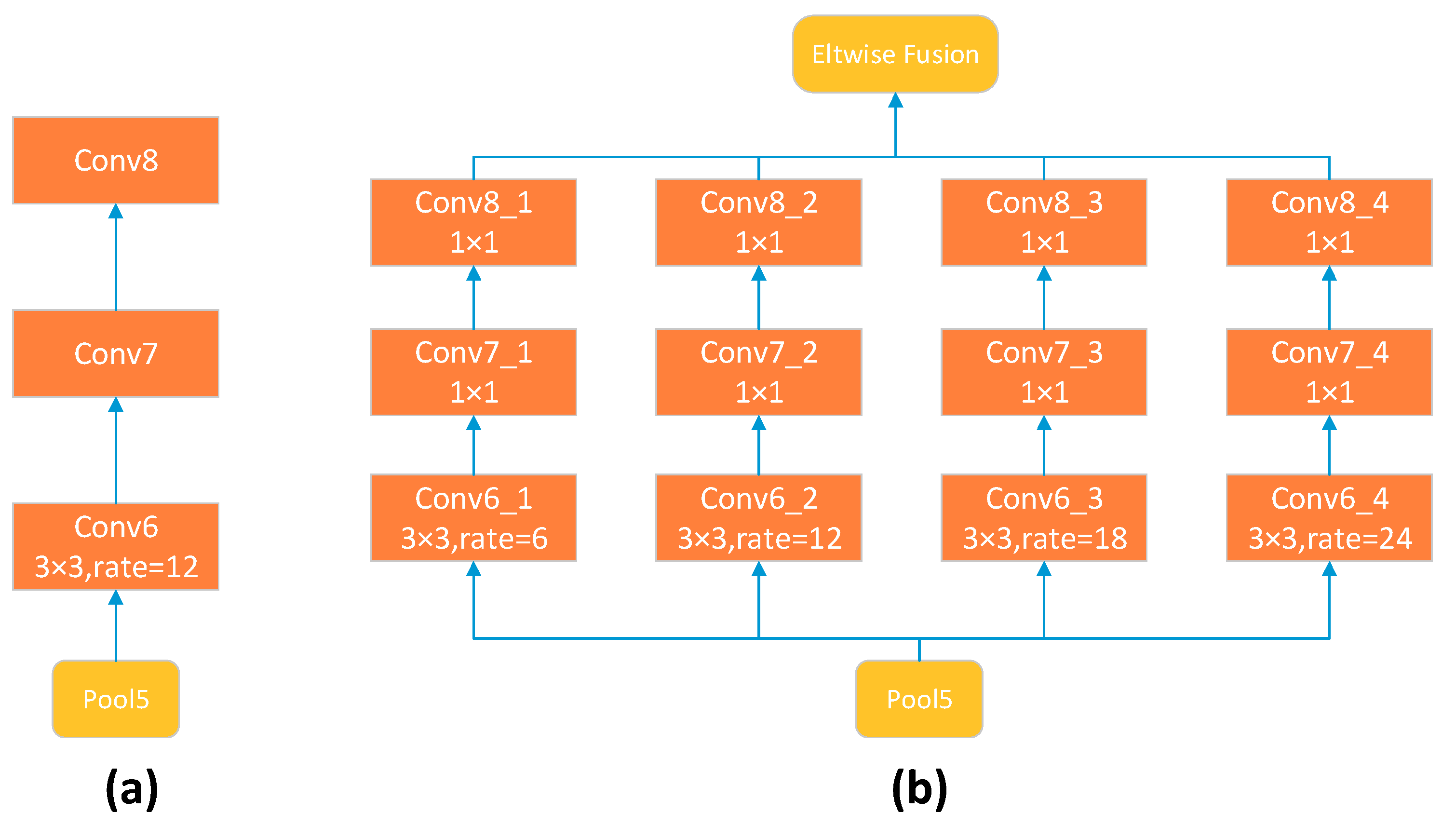
Considering that atrous convolution rates could affect the classification results, we have experimented with LargeFOV and ASPP schemes. As shown in Figure 10, ASPP for VGG-16 uses several parallel Conv6-Conv7-Conv8 branches. Each branch uses a 3 × 3 kernel; however, the atrous rates r in the “Conv6” step vary to capture objects of different sizes. In

Table 8. Effect of LargeFOV, ASPP-S and ASPP-L on the Vaihingen dataset.

Approach	Overall Accuracy
LargeFOV	84.39
ASPP-S	86.17
ASPP-L	87.78

, we report results, obtained with several settings: (1) LargeFOV, having a single branch with r = 12; (2) ASPP-S, with four branches and smaller atrous rates (r = 2, 4, 8, and 12); and (3) ASPP-L, with four branches and larger rates (r = 6, 12, 18, and 24). In Figure 11, the ASPP-L model with multiple large FOVs can capture complex objects, such as trees and buildings, better than LargeFOV and ASPP-L at multiple scales.

5.3. Accuracy Impact Factor of Different Classes

As shown in Table 2, the classification accuracy of all classes improves after training data augmentation. The best-performing class is “building”, at nearly 20% above “car” and more than 10% higher than “low vegetation”. We count both the original and augmented sample sizes of training data in

Table 9. Training sample size.

Class	Impervious Surface	Building	Low Vegetation	Tree	Car
Original Training Sample Size	645	609	1156	1160	807
Augmented Sample Size	1511	2347	583	2502	1051
Total Size	2161	2956	1739	3062	1858

to determine the impact of augmented training sample size on accuracy. In the two lowest-accuracy classes, “car” and “low vegetation”, the augmented sample size of the car class is much greater than that of low vegetation; moreover, the accuracy improvement of class “car” is better than that of “low vegetation”.

When classifying remote sensing imagery, small object classification is particularly challenging due to the class imbalance between the small object class and other classes. The car class is often mislabeled as an impervious surface, as cars in the images are of various colors, with dark-colored cars appearing similar to a shadowed road. Additionally, cars contain significantly fewer pixels than other classes. After multiple pooling and downsampling layers, the spatial resolution of the car class feature maps reduces to very low values, which might lead to this class being confused with other classes.

The distribution of the low vegetation class is scattered around other classes in an image and contains fewer large contiguous areas than other classes, e.g., impervious surface. Hence, the chances of boundary pixels of low-vegetation being confused with other classes are raised.

There are generally two kinds of classes in the Vaihingen dataset. One contains regularly shaped objects, e.g., cars, trees and buildings. Other objects, such as those with impervious surfaces and low vegetation, to some extent resemble a background, i.e., they do not have regular shapes. The selective search method that we applied is good at augmenting the former. In Table 2, we observed that the accuracy of the tree class improved by 3.17% and the accuracy of the car class improved by 2.61%.

We have also experimented with augmentation in different classes, with results shown in

Table 10. Result of augmentation in different classes.

Augmented Class	Imp. Surf.	Building	Low Veg.	Tree	Car	F1-Score	Average Recall	Overall Accuracy
Car	89.41	91.74	79.31	84.25	74.14	85.12	85.41	86.61
Low Veg.	89.40	91.71	80.09	84.21	71.53	85.29	85.72	87.06
Car + Low Veg.	89.43	91.72	80.19	84.24	74.07	85.36	85.99	87.38
All Classes	91.03	92.94	80.13	87.25	74.12	86.84	87.06	88.13

. We chose the two lowest-accuracy classes of “car” and “low vegetation” to perform the experiment. The result shows no interaction between different classes in accuracy improvement. The augmented classes are independent; all classes should be augmented to achieve a higher overall accuracy.

5.4. Applications and Limitations of Our Approach

Our proposed method makes pixel-wise classification practically feasible for very high-resolution urban remote sensing and results in a high classification accuracy. The proposed pre-segmentation and selective search method are natural and easy to implement and embed into an existing system. The ASPP network source code we used and the trained weights have been publicly released. The end-users can easily perform training data augmentation and ASPP networks in series in the training stage, while the coarse result will be refined by fully connected CRFs in the testing stage.

The network of our proposed method is based on a VGG16 architecture, which is a very large model designed for multi-class classification. It contains numerous parameters and requires time-consuming inference. As a result, it is unusable for mobile or battery-powered real-time applications that require processing images at rates higher than 10 fps [62].

Our approach is limited in two aspects. First, it needs a large number of high-quality ground truth labels for model training that relies on professional and experienced interpreters and a large amount of manual processing. Second, a significant amount of GPU memory is required due to atrous convolution.

In this paper, we apply a single neural network to pixel-wise classification. Ensemble learning methods train several individual models, and use certain rules to combine them to make predictions. The ensemble learning methods have gained popularity due to superior prediction performance in practice. Studies showed that combining multiple pixel-wise classification networks is beneficial to reducing the bias of individual models, both when using the same architecture with different initializations and when using different model architectures with identical initializations [48,63].

6. Conclusions

In this paper, we propose a three-step method for pixel-wise classification of high-resolution remote sensing imagery using a deep neural network. More specifically, our method has the following novel features: (1) adopting training augmentation before training, using both a graph-based unsupervised segmentation method and a selective search objectness proposal method; (2) using a fully convolutional network with atrous kernels for dense feature extraction to encode objects and the image context at multiple scales; and (3) using fully connected CRFs aiming at producing semantically accurate predictions and detailed segmentation maps after segmentation. Experiments on well-known high-resolution remote sensing datasets and state-of-the-art pixel-wise classification methods demonstrate the effectiveness of our proposed method. We also compare the classification results of different training crop sizes and atrous convolution kernel sizes. The larger training crop sizes and atrous rates achieve higher accuracy. Under the same conditions, our method achieves better overall accuracy and the average F1-score than the state-of-the-art methods when applied to the Vaihingen dataset.

Although CNN-based models attain the state-of-the-art results for pixel-wise image classification, their accuracy has reached a certain limit, with further improvements of classification quality probably being small. Nevertheless, there are several promising directions for future research. Ensemble learning is a method for generating multiple versions of a predictor network and using them to obtain an aggregated prediction, improving a single network performance. Another possible direction is applying a semi-supervised learning method such as Generative Adversarial Networks (GANs). The existing CNN-based models used in remote sensing are highly sensitive to satellites having different spatial resolution and sensors. In addition, a large amount of unlabeled satellite imagery of the world is available for further analysis. Hence, exploring improved approaches to using such unlabeled datasets becomes an important direction for further research.