Structured Knowledge Base as Prior Knowledge to Improve Urban Data Analysis

Abstract

Urban computing at present often relies on a large number of manually extracted features. This may require a considerable amount of feature engineering, and the procedure may miss certain hidden features and relationships among data items. In this paper, we propose a method to use structured prior knowledge in the form of knowledge graphs to improve the precision and interpretability in applications such as optimal store placement and traffic accident inference. Specifically, we integrate sub-graph feature extraction, sub-knowledge graph gated neural networks, and kernel-based knowledge graph convolutional neural networks as ways of incorporating large urban knowledge graphs into a fully end-to-end learning system. Experiments using data from several large cities showed that our method outperforms the baseline methods.

1. Introduction

Nowadays, applications of urban computing often rely on manual feature engineering tasks, which may lead to some latent features being overlooked. For example, it is usually necessary to construct and combine some complex features for machine learning tasks in urban computing. However, the complexity of applications and the different modalities of urban data make the feature construction task extremely challenging. Moreover, most learning-based approaches cannot provide explanations of the prediction results. Data generated from sensors and social media in cities contain millions of concepts that are understood by humans. Each region in a large city contains some hidden and inherent knowledge (e.g., demographics, points of interest, and so on). However, when shown only a few items of knowledge pertaining to a region, humans can make a satisfactory assessment of the area. On the contrary, modern learning-based approaches usually require thousands of labeled instances with complicated feature engineering. A combination of prior urban knowledge and available approaches are used for this.

Recently, structured knowledge representation, such as knowledge graphs [1,2], has already an played important role in search engines. Urban knowledge graphs generated from historical experience, geography, and common sense play an unexpected role in practical applications. For instance, Figure 1 illustrates how we might use prior knowledge of a region in the optimal store placement problem. If we want to open a new restaurant, we might know the target region’s function type (e.g., business area, range of rent), and that it is near a subway station (transportation), a university, a film center, and an information plaza (potential consumers), where this information may vary slightly over a relatively long period of time. As s result, we can pre-estimate that this region may be a suitable place for a new store before feeding these data into a machine learning model. We make this decision by first recalling knowledge (most prime locations have convenient transportation and a large number of consumers) and reasoning (this place has similar conditions to other prime locations). We can easily classify a region as suitable or not with only a limited amount of information.

In this paper, we exploit structured urban knowledge and reasoning to solve practical problems in urban computing. A number of studies have lately been devoted to building a knowledge graph (KG) that can be useful for machine learning, such as the Never Ending Image Learner [3], the Never Ending Language Learner [4], WordNet [5], Wikidata [6], and ConceptNet5 [7]. However, most of these KGs are noisy and contain little relevant urban knowledge. Therefore, we build our urban-specific KG from both raw data and existing knowledge bases. However, effectively extracting features from the graph persists as a problem.

To tackle a practical urban computing problem, we need to retrieve three kinds of knowledge from an urban KG: (1) the definition of the problem (e.g., what is a good location for a store?); (2) the measurement of the problem (e.g., why does this store attract more consumers?); (3) specific knowledge of the location (e.g., what feature does this location have?). A considerable amount of research is available on graph feature extraction. We classify features into three major parts: (1) Global features, which usually contain the global information of a graph. Random work-based approaches, such as the path ranking algorithm [8] and sub-graph feature extraction (SFE) [9] can easily generate features from graphs given two nodes; (2) Propagation features, which usually learn evidence between nodes conditional on the type of relations. For example, the gated graph neural network (GGNN) [10], which takes an arbitrary graph as input and learns how to propagate information given the annotation specific to the task; (3) Local features, which usually represent node-specific features. Graph convolution neural network (GCNN) [11] learn convolutional neural networks for arbitrary graphs based on kernels.

Our work improves on the above models, and adapts an end-to-end graph neural network to the urban computing problem. We propose an urban knowledge graph neural network (UKG-NN) that uses features from raw urban data and graphical features extracted from an urban KG. The SFE first is used to extract global features from the graph to obtain the definition of the problem. Following this, for each region node (node represented as a task-specific region) in an urban KG, we extract sub-graphs and use them as inputs for the GGNN to obtain knowledge of the measurement of the problem. Node-specific features are extracted based on graph kernels that represent the specific knowledge of location. Finally, we feed the three kinds of graph features and features from raw data into a neural network. We show how our UKG-NN model is effective at reasoning about concepts to improve urban computing tasks. Importantly, our model can provide some types of explanations by following the manner of the propagation of information in the graph.

The major contributions of this work are as follows:

(1)

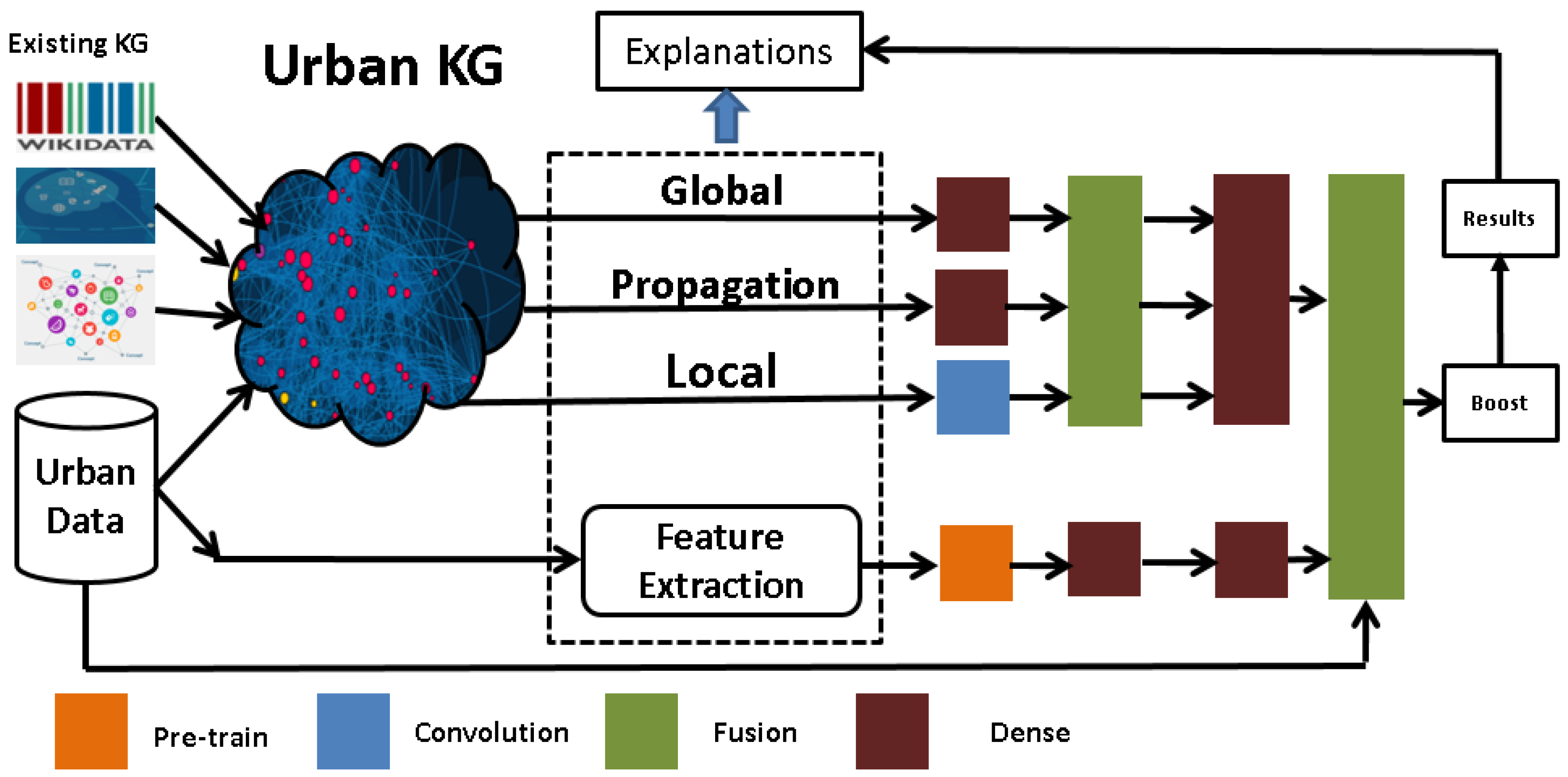
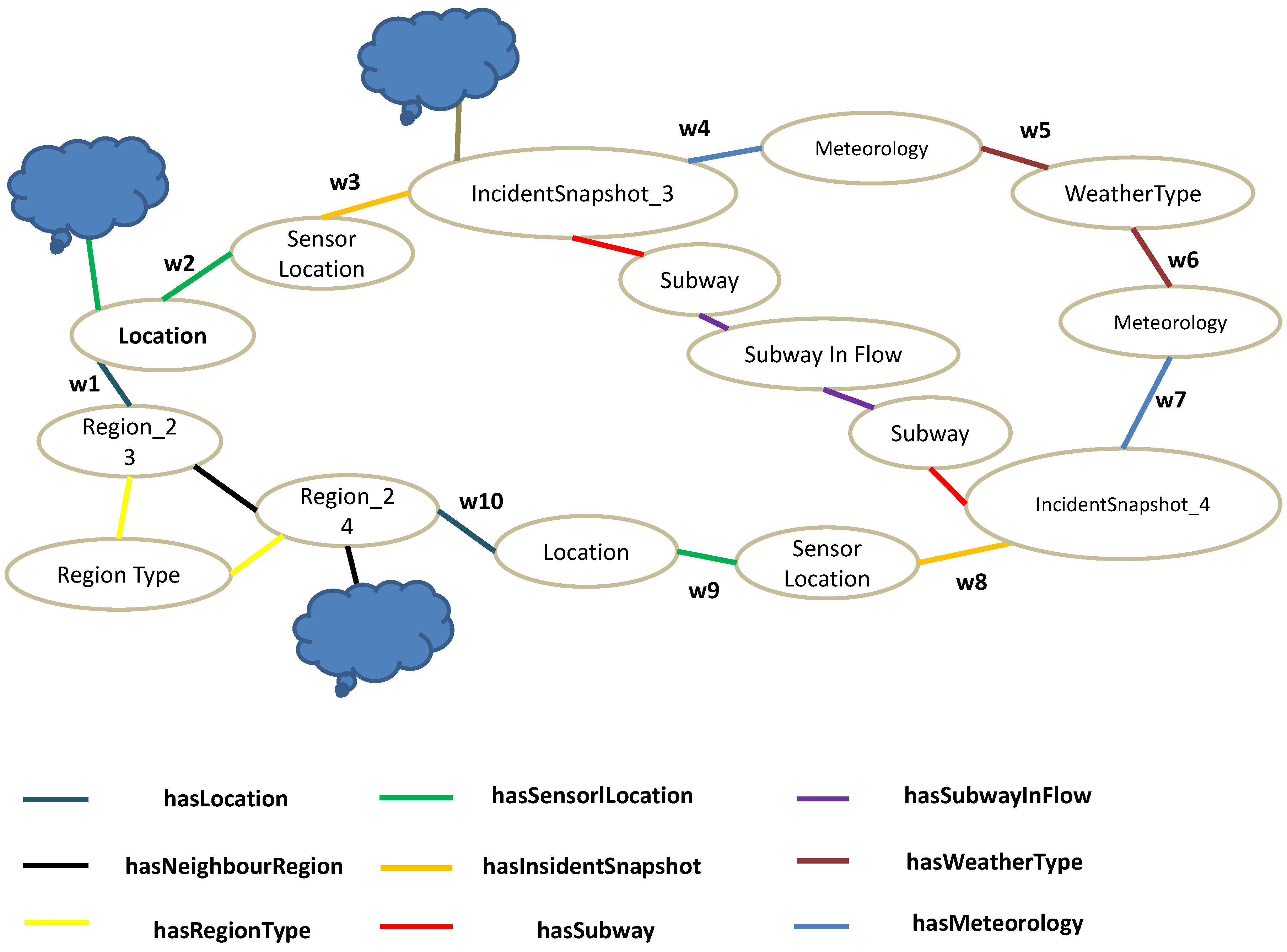
We propose a method to learn the structured knowledge representation from raw urban data and build an urban knowledge graph containing domain prior knowledge that is helpful for decision-making when there are few instances and may help improve the prediction of other applications by transfer learning. UKG-NN employs convolution-based neural network by considering global, propagation-specific, and locale-specific features automatically generated from an urban knowledge graph as well as manually extracted features from raw urban data.

(2)

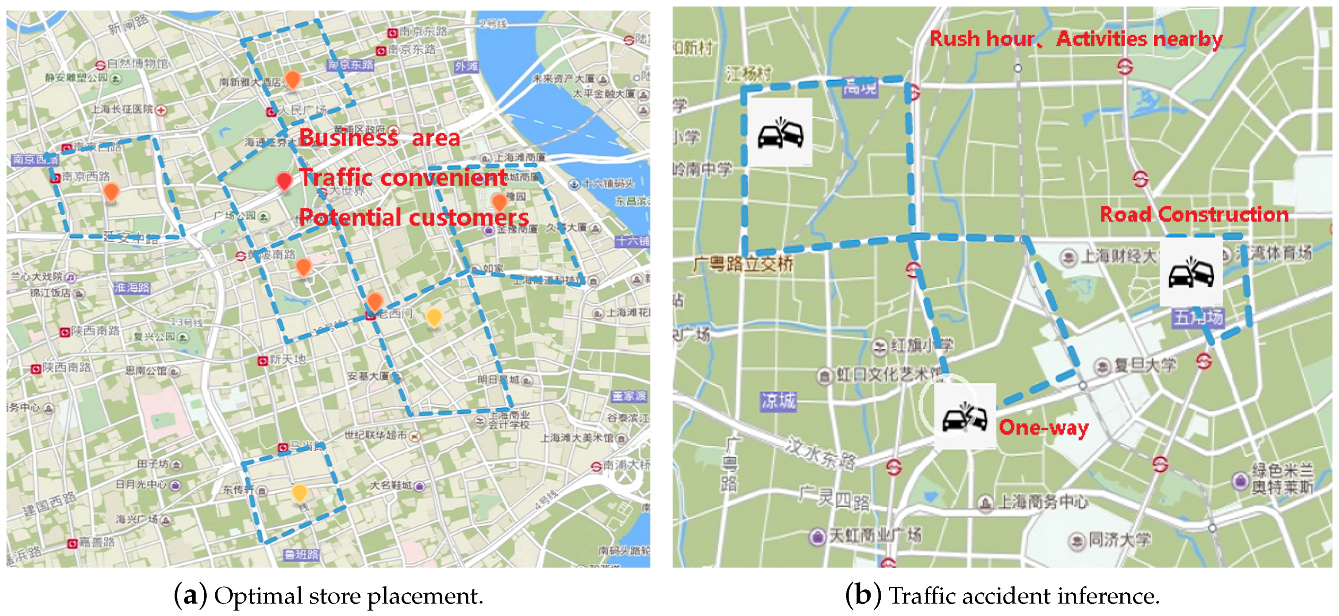
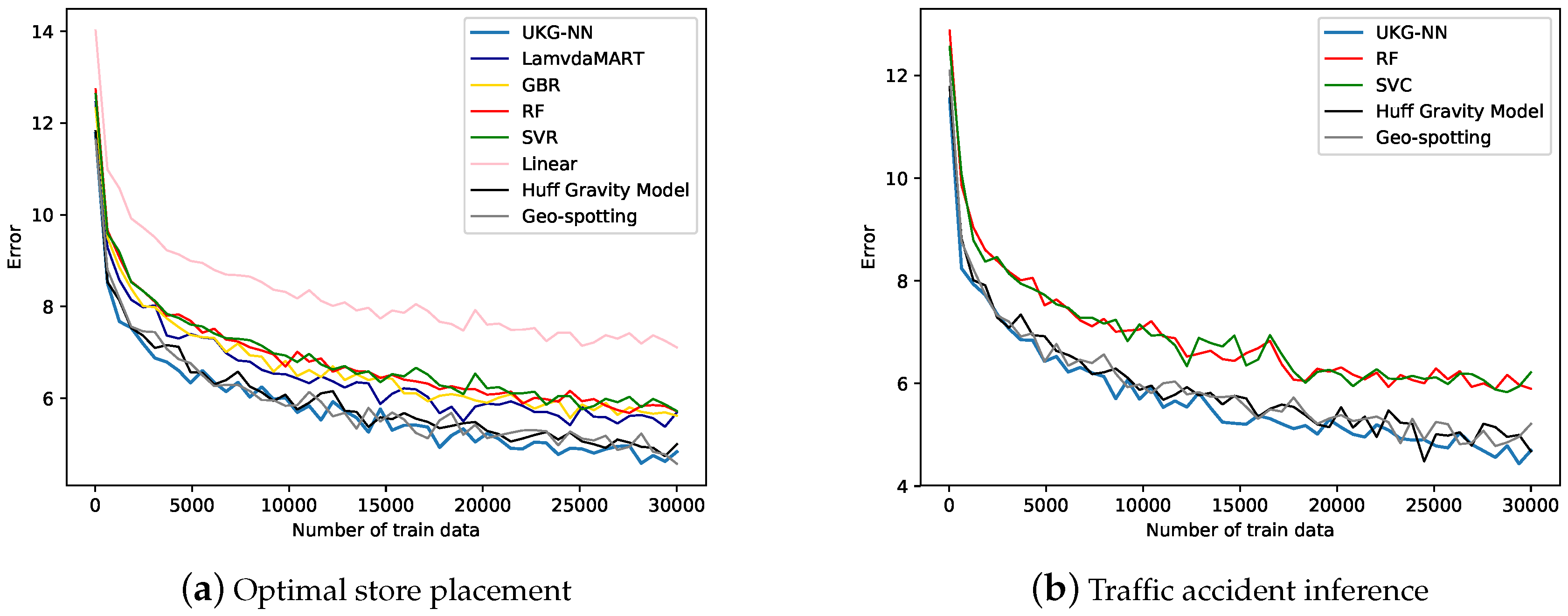
We apply the UKG-NN to optimal store placement and traffic accident inference using a noisy urban knowledge graph and manually extracted features.

(3)

The UKG-NN has the ability to explain some results of store placement and traffic accident inference as model interpretability is a requirement in many applications in which crucial decisions are made by users relying on a model’s outputs.

(4)

We evaluated our method using real user comments, taxicabs, meteorological data, and human flow data in Shanghai. The results showed that our approach outperforms the baseline methods.

2. Related Work

2.1. Urban Computing

In recent years, many applications have been proposed for different scenarios of urban data analysis, including transportation, the environment, energy, society, the economy, and public safety and security [12,13,14,15,16,17,18]. For example, a number of researchers have studied the store placement problem by focusing on various techniques, such as multiple regression discriminate analysis, spatial interaction models, and so on [19]. The spatial interaction model is based on the assumption that the strength of the interaction between positions decreases with their distance and the availability of locations increases with the strength of use and the proximity of complementary, temporally arranged positions [20,21]. However, locations cannot only attract residents near it. Multiple regression discriminant analysis [22] is location analysis that has been employed to produce a series of sales forecasts for both new and existing stores. Specifically, Ref. [23] studied the predictive power of various machine learning features on the popularity of retail stores in a city using a dataset collected from the Foursquare mall in New York. Ref. [24] proposed “Antenna Virtual Placement” (AVP), a method to geolocate mobile devices according to their connections to Base Transceiver Station (BTS), which have implications for the design of applications like recommendation of places and routes, retail store placement and so on. Ref. [25] studied an analytical approach to selecting expansion locations for retailers selling add-on products whose demand is derived from the demand of another base product. Ref. [26] employed the “Retail Gravity Model” to cultivate retail crucial variables, for example, supply chain and operation management, etc that can assist the site selection decisions of fashion retailers in Hong Kong. Ref. [27] used regional relevance analysis and human mobility construction to establish the feature values of retail store recommendation. Ref. [28] focused on locating ambulance stations by using real traffic information to minimize the average travel time to service emergency requests. On the other hand, a large number of researchers have proposed a number of methods by analyzing traffic accidents [29,30]. These focus on hotspot detection in terms of traffic accidents. Past work on finding optimal location and traffic accident inference did not consider structured urban knowledge, and cannot explain the results of the prediction.

2.2. Knowledge Graph

Learning a knowledge graph and using it for machine learning tasks has been of interest to recent researchers [31]. For example, Ref. [32] collected a knowledge base and queried it for first-order probabilistic reasoning to predict affordances. However, none of these approaches involves learning in an end-to-end manner, and the propagation model on the graph is mostly handcrafted. Ref. [9] defined a simpler algorithm for generating feature matrices from graphs called the SFE. Ref. [10] studied feature learning techniques for graph-structured inputs and modified them to use gated recurrent units and modern optimization techniques. They then extended this to output sequences called GGNN. Ref. [11] presented a general approach to extract locally connected regions from graphs. Our work improves on this model and uses end-to-end graph neural networks to construct features from an urban KG.

3. Approach

3.1. Overview

As Figure 2 shows, we first preprocess raw urban data and construct a structured data representation (urban KG) of urban data using a combination of out existing external KGs (e.g., Wikidata, ConecptNet5, and so on) based on a pre-defined urban KG OWL (Web Ontology Language). Then, global, propagation-specific, and local-specific features are automatically generated from the urban KG and fed into the neural network. We also construct several simple manual features and feed them into the neural network. After several pre-train iterations, dense net, and a confusion layer, we get the final results. The global, propagation-specific features can help explain the prediction results.

3.2. Notations and Problem Formulation

Definition 1 (Region).

In this study, we partition a city into I regions based on the road network [33].

Using these raw data and external KG, urban KG $G=(V,E)$ is constructed. Manual features $F_{i_t}$, $i\in I$ at the tth time interval are extracted for all I regions. We use consumer number $y_{i_t}^{(1)}$ in each region as the measurement of optimal store placement. We use traffic accident occurrence $y_{t_i}^{(2)}\in \{0,1\}$ as the measurement of traffic accident inference.

Problem 1.

Define $f_{i_t}^{(1)}\in F_{i_t}$ as store placement-related feature sets; $I_l$ and $I_u$ are the label region set and the unlabeled region set of optimal store placement, respectively, $I=I_l\cup I_u$, given historical observation $\{f_{i_t}^{(1)}|i=0,1,2,\dots ,n-1$, $i\in I_l\}$, and G, we need to predict $\{y_{i_t}^{(1)}$, $i\in I_u,t=n\}$.

Problem 2.

Given $f_{i_t}^{(2)}\in F_{i_t}$ as the traffic accident inference-related feature sets and historical observation $\{f_{i_t}^{(2)}|i=0,1,2,\dots ,n-1$, $i\in I\},$ and G, we need to predict $\{y_{i_t}^{(2)}$, $i\in I,t=n\}$.

As Figure 3 depicts, the predictions of our approaches including optimal store placement and traffic accident inference can be easily mapped and displayed on the city maps to help the smart cities admin for decision-making. Moreover, some supplementary information (derived from Urban KG) can explain the reasons for the predictions.

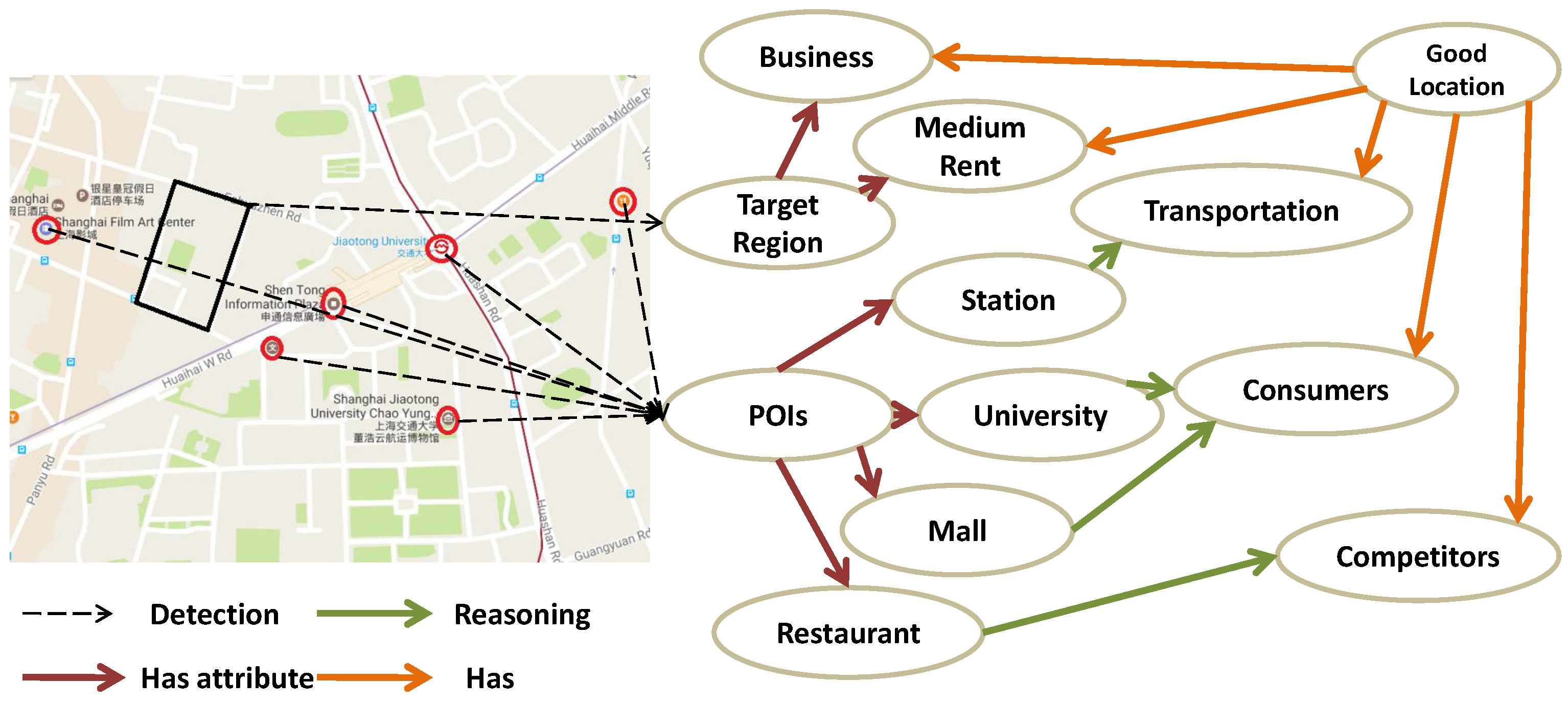
3.3. Urban Knowledge Graph

We preprocess the raw urban data to obtain raw data for each region. Based on the urban OWL, we discretize and semantically process the data. For example, given the real estate price p of region $i\in I$, we discretize the data into triples $\{Regio{n}_i$, Has_Real_Estate_Price, RealEstateHigh (if p > 60,000)}. The triples are connected and contribute to the urban KG. We build a preliminary urban KG from those raw urban data, and then collect new nodes in the external KG that are not in our output label by including ones that directly connect to our output labels and, thus, are likely to be relevant; we add these nodes to a combined graph. We then take all edges between these nodes and add them to our combined graph. Moreover, we also consider the difference of shop locations and do spatial analysis carried out in the GIS environment as an element of creating the urban knowledge base in the city. All the locations of shops are added in the KG as attribute nodes. Finally, we construct the urban KG, which is used for auto-graph feature extraction in Section 3.5.

3.4. Manual Feature Extraction

With the raw urban data, we also manually construct some simple features.

Function of the region. The most prominent Point of Interest (POI) category $f_f$ of the region itself and its surroundings is used to denote the function of the region.

Traffic convenience. The number of buses and subway stations $f_t$ are used to denote traffic convenience.

Real estate price nearby. This is the average price $f_e$ of the nearest five pieces of real estate within 2 km, and is used to estimate price.

Popularity of specific area category. The set of all POIs of category C is defined as $P_C$. Then, the popularity of a specific area category is the average number of consumers for the category $C^{{}^{\prime }}$ over all POIs in $P_C$, and its region function is $f_f$. Formally, $f_p=\frac{{\sum }_{p\in P^{{}^{\prime }}}Cum(p)}{|P^{{}^{\prime }}|}{P}^{{}^{\prime }}=\{p|f_f=C^{{}^{\prime }},p\in P\}$, where $cum(p)$ is the number of consumers of POI p.

Competition. We define the number of POIs belonging to category C in region i as $N_c(i)$, and the total number of POIs in i is $N(i)$. Then, competition is defined as the ratio of $N_c(i)$ to $N(i)$, which is $f_c=\frac{N_c(i)}{N(i)}$.

Area popularity. Consumers at places in POI j, $j\in i$ are potential consumers for a new store at i. The popularity of an area i is defined as $f_a={\sum }_{p\in j}cum(p)$.

Specifically, $f_{i_t}^{(1)}=\{f_f,f_t,f_e,f_p,f_c,f_a\}$, $f_{i_t}^{(2)}=\{f_f,f_t,f_a\}$.

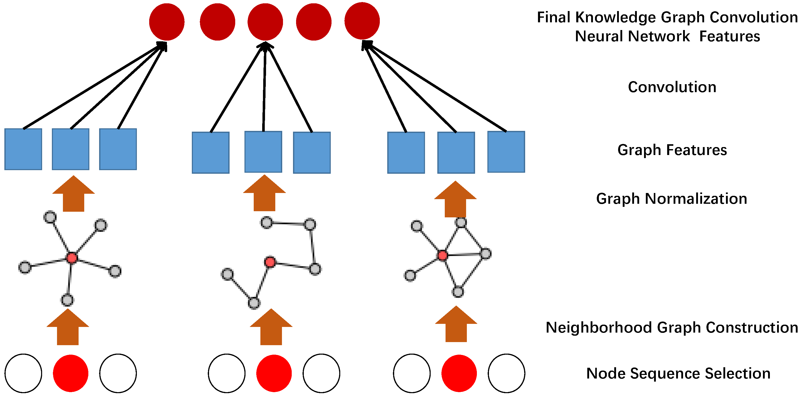
3.5. Graph Feature Extraction

Sub-Graph Feature Extraction (SFE). Given the urban KG G, we adopt SFE to obtain global knowledge. The node in G is first classified into categories $G=\{A_0,A_1,A_2,\dots ,A_n\}$ based on problems. For example, two category based the node with attribute 0 (no accident) and 1 (accident) for the task of traffic accident inference. Then, for the node $v_i$ with the region type $g_i$, we compute the feature path of all nodes in the same category $g_i$. Specifically, with node $v_i$, $H_g=concat(sfe(v_i,v_o),sfe(v_i,v_1),\dots ,sfe(v_i,v_j),\dots ,sfe(v_i,v_n))$ where $v_j$ and $v_i$ belong to the same category, $i\ne j$, n is the total number of nodes in the category containing i, where $sfe(v_i,v_j)$ computes the feature matrices from the graph through the path from $v_i$ to $v_j$. These features represent the meaning of the definition of the problem. Following this, the extracted features $H_g$ are fed into a two-layer fully connected neural network:

$$H_g^{(1)}=f(W_g^{(1)}{H}_g+b_g^{(1)}),$$

$$H_g^{(2)}=f(W_g^{(2)}{H}_g^{(1)}+b_g^{(2)}),$$

where $f(.)$ is the $relu$ function(e.g., $f(.)=max(0,x)$ ).

Sub-Knowledge Graph Gated Neural Network (s-GGNN). In contrast to the SFE, we use the sub-graph of G to extract features because the scale of the graph is very large. We generate sub-graphs $g_i$ for each region-type node i, where all nodes and edges farther than $\gamma$ are removed. For each node in graph $g_i$, we have a hidden state representation $h_v^t$ at every time step t. We start at $t=0$ with initial hidden states $x_v$ that depends on the problem. For instance, to learn graph reachability, this might be a two-bit vector that indicates whether a node is the source or the destination node. We then use the structure of our graph, encoded in matrix A, to retrieve the hidden states of adjacent nodes based on their edge types. The hidden states are then updated by a gated update module similar to an LSTM. After T time steps of the propagation network, our final hidden states are obtained. The node-level outputs can then simply be computed as $o_v=g(h_v^T,x_v)$, where g is a fully connected network, the output network, and, xv is the original annotation for the node. $H_p=o_o,o_1,\dots o_v,\dots o_m$, where m is the total number of nodes of $g_i$. Following this, the extracted features $F_G$ are fed into a two-layer fully connected neural network:

$$H_p^{(1)}=f(W_p^{(1)}{H}_p+b_p^{(1)}),$$

$$H_p^{(2)}=f(W_p^{(2)}{H}_p^{(1)}+b_p^{(2)}).$$

Kernel-Based Knowledge Graph Convolution Neural Network (GCNN).Figure 4 illustrates the Knowledge Graph Convolution Neural Network architecture. Given sub-graphs $g_i$ for each region-type node i, a receptive field needs to be constructed. The nodes of the neighborhood are candidates for the receptive field. Given as inputs a node v and the size of the receptive field k, the system performs a breadth-first search, exploring vertices with increasing distance from v, and adds these vertices to set N. If the number of collected nodes is smaller than k, the one-neighborhood of the vertices most recently added to N is collected, and so on, until at least k vertices are in N or there are no more neighbors to add. Note that, at this time, the size of N is possibly different from that of k.

The receptive field for a node is constructed by normalizing the neighborhood assembled in the previous step. The normalization imposes an order on the nodes of the neighborhood graph to map from the unordered graph space to a vector space with a linear order. The basic idea is to leverage graph labeling procedures that assign nodes of two graphs to a similar relative position in the respective adjacency matrices if and only if their structural roles within the graphs are similar. Finally, we obtain the local feature of the $H_l$ node i and feed it into a two layer convolution network:

$$H_l^{(1)}=g(W_l^{(1)}\ast H_l+b_l^{(1)}),$$

$$H_l^{(2)}=g(W_l^{(2)}\ast H_l^{(1)}+b_l^{(2)}),$$

where * denotes the convolution, $g(.):=max(0,z)$ [34].

3.6. Model

To incorporate the features of the graph into a regression task pipeline, we simply concatenate these three kinds of features with an early fusion layer to capture the global, propagation, and local patterns together. The early fusion layer can be written as

$$H^{(3)}=f(W_g^{(3)}\ast H_g^{((2))}+W_p^{(3)}\ast H_p^{((2))}+W_l^{(3)}\ast H_l^{((2))}+b^{(3)}).$$

Afterwards, we stack a fully connected layer. For the manual extraction of features, we first pretrain them on a denoise autoencoder [35]. The hidden representations are then connected with two fully connected layers with $relu$ as the activation function. Finally, all features are fed into a late fusion layer that is more adept at fusing data from different domains. In our implementation, we used external factors (i.e., function of the region ) as global features. Late fusion can be written as

$${\widehat{Y}}_r=f(W^{(5)}\ast H^{(4)}+W^{(5)}\ast Z+W_G^{(5)}\ast G_r+b^{(5)}),$$

where $G_r$ is the global feature vector of region r, Z is output of three fully connected layers from the manually extracted feature vector, and ${\widehat{Y}}_r$ is the predicted tensor. We use the mean squared error for the regression task and cross-entry error for the classification task as the loss function. To improve robustness and get better results, we adopt boosting methods using Xgboost [36].

4. Experiments

4.1. Settings

4.1.1. Datasets

We used real urban data from Shanghai, including traffic and weather, from 1 March 2015 to 1 March 2016 [37] and using the Baidu API. We partitioned the Shanghai city into 2135 regions. For the optimal store placement task, we used desensitized user location data from China Telecom near a POI as consumer data. We treated the records that were stable in the POI for more than half an hour as consumers. We used the total number of consumers in the previous two months as to measure whether a given store was considered attractive. We used two categories of stores, express inns and coffee shops, to evaluate the performance of our framework. For each category, the test data were two brands of stores to eliminate the bias of ranking and avoid over-fitting. Specifically, the training datasets were all POIs belonging to the categories “coffee shop” and “express inn” in Shanghai, except the POIs in the test data. Express inns excluded “Home-Inn” in the training set. For the traffic accident inference task, we used data from 1 March 2015 to 28 February 2016 the training set, those from 29 February 2016 as the validation set, and data from 1 March 2016 as the test set. We used the external KG data from Wikidata [38] and ConecptNet5 [39].

4.1.2. Baselines

We compared our proposed method with these eight baselines:

• Linear. We used the linear regression algorithm Lasso, where the regularization parameter were ${10}^{-2}$.
• RF. RF stands for random forests. The number of trees was 10, and the minimum number of samples required to split an internal node was set to 2. The function to measure the quality of a split was the mean squared error.
• GBR. GBR is short for gradient boosting for regression (GBR), where the loss function to be optimized was least-squares regression, and the number of boosting stages was 100.
• SVR (Support Vector Regression). The kernel function we used was also an RBF. The penalty parameter of the error term was set to 1.0, and the kernel coefficient was set to 0.1.
• SVC (Support Vector Classification). The kernel function we used was also an RBF. The penalty parameter of the error term was set to 1.5 and the kernel coefficient to 0.2.
• LambdaMART. The number of boosting stages was 100, and the learning rate was 0.1; the minimum loss required to make a further partition was 1.0.
• Huff Gravity Model. We used both manual features graph features in the Huff Gravity Model.
• Geo-spotting. We used both manual features graph features in the Geo-spotting model.

Table 1. Features of each baseline model.

Baselines	Manual Features	Graph Features
Linear	All	GCNN + SFE + s-GGNN
RF	All	GCNN + SFE + s-GGNN
GBR	All	GCNN + SFE + s-GGNN
SVR/SVC	All	GCNN + SFE + s-GGNN
LambdaMART	All	GCNN + SFE + s-GGNN
Huff Gravity Model	All	GCNN + SFE + s-GGNN
Geo-spotting	All	GCNN + SFE + s-GGNN

shows the features of each baseline model.

4.1.3. Preprocessing

In optimal store placement, we used the min-max normalization method to scale data to the range [−1,1]. In the evaluation, we re-scaled the predicted value back to the normal values compared with the ground truth. For external factors, we used one-hot coding to transform metadata into binary vectors. For all tasks, we used the function of the region as external factors.

4.1.4. Hyperparameters

The models were implemented using Python 3.6.5. Python libraries, including Thensorflow [40] and Keras [41], were used to build our models. The convolutions of CNN used 64 filters of size $3\times 3$ each, and the batch size was 32. We adopted dropout (0.5) to avoid over-fitting. The $\gamma =300$ in the procedure of getting the sub-graph. For traffic accident inference, we set the classification threshold to 0.85.

4.1.5. Evaluation Metric

For the optimal store placement task, given a POI category or a specific brand, we first evaluated the performance of our prediction method using existing POIs belonging to the same category or brand. After we had predicted scores for each POI, we obtained a ranked list $L_P$ of regions. The ranked list $L_R$ of locations based on actual popularity (number of customers) of those POIs was also obtained. To evaluate the ranking performance of our result, we utilized the nDCG@k (Normalized Discounted Cumulative Gain) metric [42] and the nSD@k (Normalized Symmetric Difference) metric proposed in [43].

The nDCG@N is given by

$$DCG\left[n\right]=\left\{\begin{array}{ccccc}\hfill re{l}_1& if,\hfill & \hfill n& =\hfill & \hfill 1,\\ \hfill DCG[n-1]+\frac{re{l}_n}{lo{g}_{2}n},& if,\hfill & \hfill n& >=\hfill & \hfill 2.\end{array}\right.$$

The normalized symmetric difference metric provides an analysis of comparing two top-k lists. Given two top-k lists, ${\tau }_1$ and ${\tau }_2$, the normalized symmetric difference metric is defined as:

$$d\Delta ({\tau }_1,{\tau }_2)=\frac{1}{2k}|({\tau }_1/{\tau }_2)({\tau }_2/{\tau }_1)|,$$

where $d\Delta$ value is denoted by nSD@k, which is always between 0 and 1.

For the traffic accident inference task, we used the F1 measure .

4.2. Results

Performance Comparison: For the optimal store placement task, as

Table 2. Results for Starbucks and Home-Inn.

Model	Starbucks		Home-Inn
	nDCG@10	nSD@10	nDCG@10	nSD@10
Linear	0.454	0.91	0.532	0.97
RF	0.743	0.70	0.710	0.87
GBR	0.754	0.88	0.745	0.87
SVR	0.643	0.91	0.675	0.95
LambdaMART	0.762	0.81	0.734	0.67
Huff Gravity Model	0.810	0.79	0.702	0.59
Geo-spotting	0.800	0.80	0.683	0.71
Ours
UKG-NN	0.812	0.60	0.781	0.50

shows, the UKG-NN yielded better results for the optimal store placement of Starbucks and Home-Inn in nDCG@10 and nSDK@10.

For the traffic accident inference task, we predicted accidents at 9:00 a.m., 10:00 a.m., 6:00 p.m., and 7:00 p.m. on 1 March 2016 As

Table 3. Results of traffic accident inference.

Model	9:00	10:00	18:00	19:00
RF	0.56	0.54	0.53	0.44
SVC	0.53	0.53	0.58	0.64
Huff Gravity Model	0.60	0.61	0.61	0.63
Geo-spotting	0.59	0.61	0.60	0.59
Ours
UKG-NN	0.61	0.65	0.65	0.60

shows, for prediction results at 9:00 a.m., 10:00 a.m., and 6:00 p.m., the UKG-NN had better results than the baselines.

Effictiveness of Urban KG: To determine the whether the UKG-NN can learn a better model based on less data, we gradually added training data. As Figure 5 shows, with increase in the number of training samples, the error dropped rapidly compared with the baselines for both the optimal store placement and traffic accident inference tasks. The UKG-NN could even obtain better results with little training data.

Explanations of Results: For region i, we obtain prediction $y_i^{(1)}=1$ at 9:00 a.m., which meant that this region might have had a traffic accident. As

Table 4. Explanations of the resultsbased on global graph features for traffic accident inference.

Relation Path	Mean Weight
(hasNeighbourRegion, hasNeighbourRegion)	0.2
(hasLocation, hasSensorlLocation, hasInsidentSnapshot, hasMeteorology, hasWeatherType, hasMeteorology, hasIncidentSnapshot, hasSensorlLocation, hasLocation)	2.13
(hasLocation, hasSensorlLocation, hasInsidentSnapshot, hasSubway, hasSubwayInFlow, hasSubway, hasIncidentSnapshot, hasSensorlLocation, hasLocation)	1.53
(hasRegionType, hasRegionType)	1.83

shows, the path for the relation between the prediction region node and the label node with had the largest weights among relations such as “hasWeatherType”, “hasSubwayInFlow” and “hasRegionType”, which indicated the possible causes of these results. Figure 6 shows part of the nodes(entities) and paths(relations) of the graph. The mean weights of each path is the average of the weights of paths (e.g., $MeanWeight={\displaystyle \sum _{i=1}^{10}}{w}_i$).

As

Table 5. Explanations of results based on propagation graph features for traffic accident inference.

Top Weights Node	Hidden Variable
RegionType	(0.3, 0.1, 0.1, 0.5, 1.3)
WeatherType	(2.3, 2.5, 2.6, 2.5, 1.9)
SubwayInFlow	(3.3, 2.4, 2.5, 2.1, 2.9)
HumanFlow	(1.3, 1.3, 1.6, 1.5, 1.9)

shows, “WeatherType” and “SubwayInFlow” were the largest weight nodes, which indicated that these data had a relatively strong effect on the final prediction results.

The explanation of the results for the optimal store placement task is similar to the above. For region i, we obtain prediction $400<y_i^{(1)}<500$ at 8:00 p.m., which meant that this region is popular. As

Table 6. Explanations of the results based on global graph features for optimal store placement.

Relation Path	Mean Weight
(hasNeighbourRegion, hasNeighbourRegion)	8.2
(hasLocation, hasSensorlLocation, hasInsidentSnapshot, hasMeteorology, hasWeatherType, hasMeteorology, hasIncidentSnapshot, hasSensorlLocation, hasLocation)	2.13
(hasLocation, hasSensorlLocation, hasInsidentSnapshot, hasSubway, hasSubwayInFlow, hasSubway, hasIncidentSnapshot, hasSensorlLocation, hasLocation)	11.53
(hasRegionType, hasRegionType)	9.83

shows, the path for the relation between the prediction region node and the label node with had the largest weights among relations such as “hasNeighbourRegion”, “hasSubwayInFlow” and “hasRegionType”, which indicated the possible causes of these results. In fact, the subway may bring a lot of passengers, which tend to be potential customers.

As

Table 7. Explanations of results based on propagation graph features for optimal store placement.

Top Weights Node	Hidden Variable
RegionType	(5.3, 3.1, 5.1, 11.5, 3.3)
WeatherType	(1.3, 1.5, 1.6, 1.5, 1.2)
SubwayInFlow	(3.3, 2.4, 5.5, 9.1, 3.9)
HumanFlow	(7.3, 6.3, 6.6, 6.5, 6.9)

shows, “RegionType”, “HumanFlow” and “SubwayInFlow” were the largest weight nodes, which indicated that these data had a relatively strong effect on the final prediction results.

Ablation Study

To analyze the effect of varying different components of our framework, we also report the ablation test of the UKG-NN in terms of using different setups of the network. The experimental results are summarized in

Table 8. Ablation study for optimal store placement.

Model	Starbucks		Home-Inn
	nDCG@10	nSD@10	nDCG@10	nSD@10
UKG-NN	0.812	0.60	0.781	0.50
FC	0.644	0.70	0.674	0.86
FC + Boost	0.691	0.67	0.699	0.73
GCNN + FC	0.686	0.67	0.707	0.81
GCNN + SFE + FC	0.743	0.66	0.731	0.74
GCNN + SFE + s-GGNN + FC	0.781	0.62	0.760	0.55

for the optimal store placement and in

Table 9. Ablation Study for traffic accident inference.

Model	9:00 a.m.	10:00 a.m.	6:00 p.m.	7:00 p.m.
UKG-NN	0.61	0.65	0.65	0.60
FC	0.46	0.44	0.46	0.49
FC + Boost	0.49	0.49	0.47	0.51
GCNN + FC	0.45	0.49	0.48	0.52
GCNN + SFE + FC	0.55	0.50	0.51	0.55
GCNN + SFE + s-GGNN + FC	0.57	0.51	0.55	0.57

for the traffic accident inference. Generally, all three proposed strategies including Boost, GCNN, SFE, s-GGNN, and FC (Fully Connected Layer) contribute to the effectiveness of UKG-NN (integrates all methods aforementioned).

5. Conclusions

In this study, we built an urban knowledge graph containing domain prior knowledge that is helpful for decision-making such as human flow or traffic monitoring and guidance when there are few instances and may help improve the prediction of other applications by transfer learning. We proposed UKG-NN that employs convolution-based neural networks by considering global, propagation-specific, and locale-specific features automatically generated from an urban knowledge graph and manually extracted features from raw urban data. We discussed two case studies based on the implementation of our framework and obtained interesting results. In addition, we tested our proposed approach, and the results showed that it is practical, and can provide explanations for predictions as model interpretability is a requirement in many applications in which crucial decisions are made by users relying on a model’s outputs.

There are some limitations to this study, which should be addressed in future work. One major one lies in the partially missing data when constructing the urban KG. For example, some data cannot be represented in the urban KG due to a lack of the representation of OWL and a procedure for discretization. We would like to mine the data for regions more deeply and try a spatial interpolation approach in the future to reduce data loss. The adaptability of this approach to real-world circumstances will also be considered in future work. Some visual analytics functions will be added to our ongoing demonstration system. By presenting similar historical circumstances or forecasting results according to different features, the system will be able to provide more information for flexible decision-making. We are also investigating a new model that utilizes data from similar historical circumstances to understand the underlying semantics. We plan to apply our approach to additional applications such as urban smog prediction and urban road planning. Moreover, we aim to study the distribution of our framework to enable it to process very large amounts of data.

References

1. Gomez-Perez, J.M.; Pan, J.Z.; Vetere, G.; Wu, H. Enterprise KnowledgeGraph: An Introduction. In Exploiting Linked Data and Knowledge Graphs in Large Organisations; Springer: Heidelberg/Berlin, Germany, 2017; pp. 1–14. [Google Scholar]
2. Pan, J.Z.; Vetere, G.; Gomez-Perez, J.M.; Wu, H. Exploiting Linked Data and Knowledge Graphs in Large Organisations; Springer: Heidelberg/Berlin, Germany, 2017. [Google Scholar]
3. Chen, X.; Shrivastava, A.; Gupta, A. Neil: Extracting visual knowledge from web data. In Proceedings of the IEEE International Conference on Computer Vision, Sydney, Australia, 1–8 December 2013; pp. 1409–1416. [Google Scholar]
4. Mitchell, T.; Fredkin, E. Never ending language learning. In Proceedings of the 2014 IEEE International Conference on Big Data, Washington, DC, USA, 27–30 October 2014. [Google Scholar]
5. Miller, G.A. WordNet: A lexical database for English. Commun. ACM 1995, 38, 39–41. [Google Scholar] [CrossRef]
6. Vrandečić, D.; Krötzsch, M. Wikidata: A free collaborative knowledgebase. Commun. ACM 2014, 57, 78–85. [Google Scholar] [CrossRef]
7. Liu, H.; Singh, P. ConceptNet—A practical commonsense reasoning tool-kit. BT Technol. J. 2004, 22, 211–226. [Google Scholar] [CrossRef]
8. Lao, N.; Minkov, E.; Cohen, W.W. Learning Relational Features with Backward Random Walks; Atlantic Container Line: Westfield, NJ, USA, 2015; pp. 666–675. [Google Scholar]
9. Gardner, M.; Mitchell, T.M. Efficient and Expressive Knowledge Base Completion Using Subgraph Feature Extraction. In Proceedings of the 2015 Conference on Empirical Methods in Natural Language Processing, Lisbon, Portugal, 17–21 September 2015; pp. 1488–1498. [Google Scholar]
10. Li, Y.; Tarlow, D.; Brockschmidt, M.; Zemel, R. Gated graph sequence neural networks. arXiv, 2015; arXiv:1511.05493. [Google Scholar]
11. Niepert, M.; Ahmed, M.; Kutzkov, K. Learning convolutional neural networks for graphs. In Proceedings of the 33rd Annual International Conference on Machine Learning, Orlando, FL, USA, 4–8 December 2017. [Google Scholar]
12. Lau, B.P.L.; Wijerathne, N.; Ng, B.K.K.; Yuen, C. Sensor fusion for public space utilization monitoring in a smart city. IEEE Int. Things J. 2018, 5, 473–481. [Google Scholar] [CrossRef]
13. Zhou, Y.; Lau, B.P.L.; Yuen, C.; Tunçer, B.; Wilhelm, E. Understand Urban Human Mobility through Crowdsensed Data. arXiv, 2018; arXiv:1805.00628. [Google Scholar]
14. Zhang, N.; Chen, H.; Chen, X.; Chen, J. ELM Meets Urban Computing: Ensemble Urban Data for Smart City Application; Springer: Heidelberg/Berlin, Germany, 2016; pp. 51–63. [Google Scholar]
15. Zhang, N.; Chen, H.; Chen, J.; Chen, X. Social media meets big urban data: A case study of urban waterlogging analysis. Comput. Intell. Neurosci. 2016, 2016. [Google Scholar] [CrossRef] [PubMed]
16. Zhang, N.; Zheng, G.; Chen, H.; Chen, X.; Chen, J. Monitoring urban waterlogging disaster using social sensors. In Proceedings of the Chinese Semantic Web and Web Science Conference, Wuhan, China, 8–12 August 2014; Springer: Heidelberg/Berlin, Germany, 2014; pp. 227–236. [Google Scholar]
17. Zhang, N.; Chen, H.; Chen, X.; Chen, J. Forecasting public transit use by crowdsensing and semantic trajectory mining: Case studies. ISPRS Int. J. Geo-Inf. 2016, 5, 180. [Google Scholar] [CrossRef]
18. Zhang, N.; Chen, H.; Chen, X.; Chen, J. Semantic framework of internet of things for smart cities: Case studies. Sensors 2016, 16, 1501. [Google Scholar] [CrossRef] [PubMed]
19. Hernandez, T.; Bennison, D. The art and science of retail location decisions. Int. J. Retail Distrib. Manag. 2000, 28, 357–367. [Google Scholar] [CrossRef]
20. Kubis, A.; Hartmann, M. Analysis of location of large-area shopping centres. A probabilistic Gravity Model for the Halle–Leipzig area. Jahrbuch Regionalwissenschaft 2007, 27, 43–57. [Google Scholar] [CrossRef]
21. Xiao, X.; Yao, B.; Li, F. Optimal location queries in road network databases. In Proceedings of the 2011 IEEE 27th International Conference on Data Engineering (ICDE), Hannover, Germany, 11–16 April 2011; pp. 804–815. [Google Scholar]
22. Rogers, D. Site for store buys. New Perspect. 1997, 5, 14–17. [Google Scholar]
23. Li, Y.; Zheng, Y.; Ji, S.; Wang, W.; Gong, Z. Location selection for ambulance stations: A data-driven approach. In Proceedings of the 23rd SIGSPATIAL International Conference on Advances in Geographic Information Systems, Seattle, WA, USA, 3–6 November 2015; p. 85. [Google Scholar]
24. Graells-Garrido, E.; Peredo, O.; García, J. Sensing urban patterns with antenna mappings: The case of Santiago, Chile. Sensors 2016, 16, 1098. [Google Scholar] [CrossRef] [PubMed]
25. Huang, T.; Bergman, D.; Gopal, R. Predictive and Prescriptive Analytics for Location Selection of Add-on Retail Products. arXiv, 2018; arXiv:1804.01182. [Google Scholar]
26. Ching, W.; Chu, A.; Hin, M.; Chan, E. A Retail Gravity Model for Selecting the Optimal Store Location. In Proceedings of the 2017 World Transport Convention, Beijing, China, 3–6 June 2017. [Google Scholar]
27. Chen, T.Y.; Chen, L.C.; Chen, Y.M. Mining Location-Based Service Data for Feature Construction in Retail Store Recommendation; Springer: Heidelberg/Berlin, Germany, 2017; pp. 68–77. [Google Scholar]
28. Karamshuk, D.; Noulas, A.; Scellato, S.; Nicosia, V.; Mascolo, C. Geo-spotting: mining online location-based services for optimal retail store placement. In Proceedings of the 19th ACM SIGKDD International Conference on Knowledge Discovery and Data Mining, Chicago, IL, USA, 11–14 August 2013; pp. 793–801. [Google Scholar]
29. Xie, Z.; Yan, J. Detecting traffic accident clusters with network kernel density estimation and local spatial statistics: An integrated approach. J. Trans. Geogr. 2013, 31, 64–71. [Google Scholar] [CrossRef]
30. Bíl, M.; Andrášik, R.; Janoška, Z. Identification of hazardous road locations of traffic accidents by means of kernel density estimation and cluster significance evaluation. Accid. Anal. Prev. 2013, 55, 265–273. [Google Scholar] [CrossRef] [PubMed]
31. Malisiewicz, T.; Efros, A. Beyond Categories: The Visual Memex Model for Reasoning about Object Relationships. In Proceedings of the Advances in Neural Information Processing Systems, Vancouver, BC, Canada, 7–10 December 2009; pp. 1222–1230. [Google Scholar]
32. Zhu, Y.; Fathi, A.; Fei-Fei, L. Reasoning about Object Affordances in a Knowledge Base Representation; Springer: Heidelberg/Berlin, Germany, 2014; pp. 408–424. [Google Scholar]
33. Road Network Segementation. Available online: https://github.com/zxlzr/Segment-Maps (accessed on 5 July 2018).
34. Krizhevsky, A.; Sutskever, I.; Hinton, G.E. Imagenet classification with deep convolutional neural networks. In Proceedings of the 25th International Conference on Neural Information Processing Systems, Lake Tahoe, Nevada, 3–6 December 2012; pp. 1097–1105. [Google Scholar]
35. Bengio, Y. Learning deep architectures for AI. Found. Trends Mach. Learn. 2009, 2, 1–127. [Google Scholar] [CrossRef]
36. Chen, T.; Guestrin, C. Xgboost: A scalable tree boosting system. In Proceedings of the 22nd ACM SIGKDD International Conference on Knowledge Discovery and Data Mining, San Francisco, CA, USA, 13–17 August 2016; pp. 785–794. [Google Scholar]
37. Soda Data of Shanghai. Available online: http://soda.datashanghai.gov.cn/ (accessed on 5 July 2018).
38. Wikidata. Available online: http://www.wikidata.org (accessed on 5 July 2018).
39. ConceptNet5. Available online: http://github.com/commonsense/conceptnet5 (accessed on 5 July 2018).
40. Abadi, M.; Barham, P.; Chen, J.; Chen, Z.; Davis, A.; Dean, J.; Devin, M.; Ghemawat, S.; Irving, G.; Isard, M.; et al. TensorFlow: A System for Large-Scale Machine Learning. arXiv, 2016; arXiv:1605.08695v2. [Google Scholar]
41. Chollet, F. Keras. Available online: https://github.com/keras-team/keras (accessed on 5 July 2018).
42. Järvelin, K.; Kekäläinen, J. Cumulated gain-based evaluation of IR techniques. ACM Trans. Inf. Syst. 2002, 20, 422–446. [Google Scholar] [CrossRef] [Green Version]
43. Li, J.; Deshpande, A. Consensus answers for queries over probabilistic databases. In Proceedings of the Twenty-Eighth ACM SIGMOD-SIGACT-SIGART Symposium on Principles of Database System, Providence, RI, USA, 29 June–1 July 2009; pp. 259–268. [Google Scholar]
Figure 1. Example of how semantic knowledge of region aids store placement.
Ijgi 07 00264 g001
Figure 2. Proposed framework.
Ijgi 07 00264 g002
Figure 3. Visualization of predictions for smart cities.
Ijgi 07 00264 g003
Figure 4. Knowledge Graph Convolution Neural Network. A node sequence is selected from a graph via a graph labeling procedure. For some nodes in the sequence, a local neighborhood graph is assembled and normalized. The normalized neighborhoods are used as receptive fields and combined with existing Convolution Neural Network (CNN) components.
Ijgi 07 00264 g004
Figure 5. Effectiveness of Urban KG:error vs. number of train data.
Ijgi 07 00264 g005
Figure 6. Part of the urban knowledge graph for traffic accident inference tasks.
Ijgi 07 00264 g006