Estimating the Available Sight Distance in the Urban Environment by GIS and Numerical Computing Codes


Politecnico di Torino, Department of Environment, Land and Infrastructure Engineering (DIATI), 24, corso Duca degli Abruzzi, 10129 Torino, Italy
*
Author to whom correspondence should be addressed.
ISPRS Int. J. Geo-Inf. 2019, 8(2), 69; https://doi.org/10.3390/ijgi8020069
Submission received: 13 December 2018
/
Revised: 9 January 2019
/
Accepted: 27 January 2019
/
Published: 30 January 2019
(This article belongs to the Special Issue GIS for Safety & Security Management)
Abstract
:The available sight distance (ASD) is that part of the roadway ahead which is visible to the driver, and should be of sufficient length to allow a vehicle traveling at the designated speed to stop before reaching a stationary object in its path. It is fundamental in assessing road safety of a project or on an existing road section. Unfortunately, an accurate estimation of the available sight distance is still an issue on existing roads, above all due to the lack of information regarding the as-built condition of the infrastructure. Today, the geomatics field already offers different solutions for collecting 3D information about environments at different scales, integrating multiple sensors, but the main issue regarding existing mobile mapping systems (MMSs) is their high cost. The first part of this research focused on the use of a low-cost MMS as an alternative for obtaining 3D information about infrastructure. The obtained model can be exploited as input data of specific algorithms, both on a GIS platform and in a numerical computing environment to estimate ASD on a typical urban road. The aim of the investigation was to compare the performances of the two approaches used to evaluate the ASD, capturing the complex morphology of the urban environment.
1. Introduction
To reduce frequency and severity of crashes, road engineers are committed to protecting all road users by providing drivers with adequate sight distances from potential obstacles along the driving path [1]. According to the standards and regulations which are currently applied to new roads, drivers must have a visible space along their trajectory, called the available sight distance (ASD), which permits them to maintain control of the vehicle and to avoid collisions with unexpected objects or other road users on the carriageway.
Figure 1 shows the conceptual relationship between the ASD and crash rates (i.e., the ratio between the number of crashes per year and the average daily traffic volume) [2]. The figure shows that crash rates increase rapidly once ASDs fall below a threshold (ASDT), while they are relatively constant (i.e., insensitive) when the ASD is above the ASDT (case A).
Still conceptually, the threshold tends to increase (ASDT → ASDT’) in road sections where additional hazards may occur (Case B in Figure 1), thus shifting the curve to the right. Different curves characterize roads belonging to different categories and with traffic moving at different speeds. Figure 1 emphasizes the negative effects that inadequate ASD values have in terms of safety, and supports current standards that use sight distance analysis in the design of new infrastructures.
Some studies have highlighted the link between accident rates and insufficient ASD values [3,4,5,6]. Other authors [7] estimated that excessive speed combined with insufficient ASD could have been the cause of approximately 4% of recorded crashes, from an investigation of more than 100 km of roads affected by 500 crash events.
Recently, Harwood & Bauer [8] confirmed this conclusion. They carried out an investigation into 452 crest vertical curves on two-lane rural highways, and found that 214 presented an ASD above, and 238 below, the American Association of State Highway and Transportation Officials (AASHTO) criteria [1]. They noted the low incidence of crashes at sites where the driver could see certain features such as horizontal curves, intersections, and/or driveways ahead. In particular, in the case of crest vertical curves with hidden features the crash frequency values for both total crashes (crash/mile/year), and injury and fatal crashes were 43% and 62% higher respectively than in cases where the same features were not hidden.
An evaluation of ASD requires either in-field surveys or the use of software to analyze 3D models [9,10]. Road design software (RDS), geographic information systems (GIS) platforms, and numerical computing environments have all benefitted from the inclusion of tools for sight analysis [11,12].
Starting with digital terrain models (DTM), RDS is used to design horizontal and vertical alignments and to spatially define the new project surfaces (i.e., pavement, medians, margins, and escarpments). The DTM and the project model are analyzed to derive the ASD from vehicle trajectories, which conventionally coincide with the centerline of each lane. However, the evaluation of the ASD with RDS may be unduly affected by inaccuracies due to the impossibility of modeling obstructions such as vegetation and objects with vertical surfaces (i.e., buildings) for inclusion in a DTM. Moreover, RDS presents difficulties with model creation in the case of existing roads, because it necessitates information that can be included only after regression (i.e., real centerline alignment).
In contrast, GIS software uses digital surface models (DSMs), which are more flexible in the modeling of sight obstructions. GIS can also incorporate all kinds of geospatial data (e.g., light detection and ranging—LiDAR—and images can be used to evaluate sight obstructions), and global navigation satellite system (GNSS) receivers may be used to include vehicle trajectories defined as a set of 3D points [13,14,15].
For visibility analysis, it is necessary to build 3D geo-referenced representations of the environment with controlled accuracy. Nowadays, geomatics offers different solutions, methodologies, and technologies for collecting 3D information (one of the main research topics in photogrammetry and computer vision is the 3D reconstruction of objects in different scales).
Indeed, 3D representation is currently carried out with techniques employing active sensors, such as laser scanners, structured light systems, and passive sensors (e.g., RGB cameras). In particular, the image-based approach has been recently improved thanks to the contribution of computer vision [16,17,18], which offers automatic procedures for image orientation [19] and for the 3D reconstruction of objects [20]. With this approach, complex objects and scenes can be detected and reconstructed using sequences of images with accurate results. The main output of both approaches is a point cloud, which is a real-world digital representation (defined by points) that can be archived and subsequently interpreted. Point clouds can be further processed to represent the environment in the form of triangulated meshes, which in turn can be then analyzed by GIS software.
This paper reports the results of a research project focused on the estimation of ASD along urban roadways. Taking into account the aspects related to the generation of urban 3D models, this work proposes a low-cost solution for the acquisition of 3D data, flexible enough to obtain 3D models of the environment with the accuracy needed to perform visibility analysis. The authors explored the problems encountered in the formation of a 3D model of an urban road section used here as a case study. Sight obstructions were surveyed and included in a DSM already available in the GIS environment. Vehicle trajectories and the positioning of drivers’ line of sight were first reconstructed, and then used to calculate the ASD from the driver’s point of view; the information was then used to generate sight profiles.
The aim of this paper is to assess how effective GIS, numerical computing software, and related tools for sight analysis are when estimating the ASD, which represents a fundamental parameter used in important applications related to road safety including, for example, the setting of speed limits along road sections. It is worth noting that an estimation of the ASD from virtual 3D models leads to a dramatic reduction in the costs and risks involved, and sometimes the time required, when compared to the direct survey of this parameter in the field (the methodology employed is analogous to the algorithms described in Section 3).
2. Background
The Highway Safety Manual [21], as well as many other national standards, regards inadequate (restricted and/or limited) sight distance as a possible crash contributing factor along roadway segments, at signalized and unsignalized intersections, and along highway–rail grade crossings. It is also regarded as a contributing factor to crashes that involve pedestrians and cyclists.
The ASD is the length of road that the driver can see in front of him/her, without considering the influence of traffic (of vehicles, bikers, and pedestrians), weather, and road lighting. In road geometric analysis and design, the distance of unobstructed vision (Figure 2) is compared with the distance necessary to perform emergency stops in front of unexpected obstacles (stopping sight distance, SSD), to overtake slower vehicles (passing sight distance, PSD), and to change lanes on the carriageway at particular points such as intersections and exit ramps (change lane distance, CLD).
Other maneuvers are considered in the comparison with ASD values. In the US, for example, the decision sight distance (DSD), which is the distance required for the detection of an unexpected or otherwise difficult to perceive information source or condition in a roadway environment, is also compared to the ASD [1]. Although current standards only impose sight analyses on new constructions, it is worth noting that such analyses could be extended to existing roads that need to be improved in terms of safety.
Figure 2 provides a graphical illustration of the significance of ASD, showing the plan and vertical profile of a typical driving situation along a horizontal curve where a driver at point P is able to see all the points along the trajectory to point Q, if the sight obstruction limits the field of vision. This is the case of sight obstructions tall enough (height equal to hO,1) to obscure the part of the trajectory beyond Q (i.e., ASD=ASD1). Conversely, small sight obstructions with a height below the line of sight (hO,3) do not obstruct visibility, thus the driver can see beyond point Q (i.e., ASD>ASD1). In both cases, the evaluation of the ASD is relatively straightforward and can be carried out by referring to the plan view.
The case of an obstruction with a height close to the line of sight (hO,2) cannot be analyzed in a planar representation (either vertical or horizontal), and needs to be investigated using a 3D analysis. This analysis is also necessary in the case of a vertical and horizontal curve combination, and when multiple sight obstructions such as traffic barriers, vegetation, parked vehicles, street furniture, fences, and buildings are located along the roadside. In night-time conditions, the ASD is reduced in vertical sag curves, because the space illuminated by the vehicle headlights is shorter than the corresponding space along grades.
In Figure 2, the ASD also depends on the height of the driver’s eye above the road surface (hP), and the object height above the pavement surface (hQ) established by the road design standard as a function of the driving maneuver considered (SSD, PSD, CLD, DSD, or others according to national regulations).
As previously stated, the ASD on existing roads can be estimated using (a) direct field measurements, or (b) indirect measurements using a 3D model of the road scenario. Case (a) involves the total or partial closure of the road section to traffic for the time necessary to perform the survey, sometimes subjecting the operators to dangerous working conditions. Furthermore, the evaluation must be extremely accurate, and a lot of time and effort is necessary to gather a sufficient quantity of ASD data. Case (b) requires the acquisition and processing of geospatial data from an existing geodatabase and/or from field surveys (with static and mobile devices). Geospatial data must include 3D elements such as the pavement surface, margins, and any potential sight obstructions (trees, buildings, street furniture, etc.). The acquired data must then be treated and processed to generate the 3D model. Finally, the vehicle trajectories are reconstructed, and the ASD is evaluated at a number of points in order to achieve the desired level of accuracy.
Visibility analyses are generally conducted by tracking line of sight (LOS) from a certain point to a defined target [22,23,24,25], or by analyzing all the visible points/areas from a certain viewpoint [26] or, finally, by evaluating the visibility of a landmark from points/areas surrounding it [27,28]. However, these approaches could be expensive in terms of time and memory consumption, and, generally, do not take into account the point of view motion. Today, various software for 3D urban model management and analysis are available (i.e., LOS, Viewshed) [29,30]. However, they simply visualize the computed results, and it is not possible to extract information such as the obstruction position.
Even in the fields of space syntax and cognitive science, attempts have been made to analyze the visibility along an environment through the approaches of isovist [31,32], namely, the polygon generated by all points visible from a certain point of view, and the visibility graphs [33] by computing the intervisibility between nodes regularly distributed on a grid over the whole environment [34]. Both theories relate the spatial properties of the environment with the spatial behavior and allow extracting several numerical indexes, which describe the properties of the corresponding space from the observer point of view. However, many of these studies are aimed at a two-dimensional environment analysis, or do not take into account the observer’s motion within the environment.
3. Methodology
Following the procedure (b) indicated in the Background section, i.e., indirect measurements, ASD evaluation needs a 3D model of the road and the surrounding environment, the position(s) of the observer (i.e., the driver’s point of view), and the position of the potential obstacle identified as the target point [15]. Accuracy is required in the identification of such elements, since small variations in the dimension and position of objects within the road environment can lead to large variations in the ASD estimate values.
Within this work, a section of an existing road impossible to survey for operational reasons (it would have necessitated a temporary road closure) was analyzed. Then, in the investigation, tested data of known accuracy (i.e., orthophoto and DTM) were used for the creation of the 3D model. However, these data were not updated, and required integration by means of low-cost instruments. Figure 3 summarizes the workflow process in the generation of the DSM.
3.1. Basic Cartographic Input Data and DSM generation
The basic cartographic information was provided by the Regione Piemonte administration (Italy), and consists of:
- technical maps scale 1:1000 (edition 2014), which include details of buildings, roads, and public and private land holdings;
- colored orthophotos of the same area at a resolution of 30 cm (edition 2012), which are aerial photographs ‘ortho-rectified’ (geometrically corrected) so that the scale is uniform;
- a digital terrain model (DTM) with a grid of 5 m;
- aerial images taken from different positions, which, using a stereoscopic technique, digitally plot an object in its correct 3D spatial position; and
- a digital surface model (DSM), with a grid of 20 cm, of a small portion of the case study area.
To build an initial prototype of the 3D model (Figure 3), a basic 2D model was generated by integrating the cartographic data #1 (the technical map), the colored orthophoto #2, and the DTM #3 into a commercial GIS platform. This basic model was then integrated with objects along or near the road path through analysis of the video frames extracted with mobile mapping system (MMS) (discussed in the next section). Horizontal markings were added to the model using aerial images and the stereoscopic model (data #4).
The 3D model was then generated, using the DTM as a reference for the terrain elevation and all the entities that constitute the urban environment. The elevation point on the technical map defined the height of each element. During the construction of the model, the dynamics and variability of the environment were taken into account.
In fact, protruding or over extending vegetation can affect driver visibility. Moreover, parts of street furniture and parked vehicles are not fixed to the ground, and can occupy different positions in the urban scenario. For example, the parking stalls can only be occupied by vehicles, and this implies that the 3D models for such a scenario cannot have a corresponding reference ground truth. In this context, a sight analysis should be carried out in the context of to the most restrictive conditions.
The model was then integrated with the obstruction formed by the vehicles parked on the roadsides. Since not all the parking stalls were occupied by vehicles for the duration of the surveys, a solid obstruction was created in the model to take the most unfavorable sight conditions along the investigated road section into account. This was achieved through the extrusion of the parking lot surface (visible on the orthophoto) with a height of 1.60 m. This operation resulted in a new solid surface that was assumed equivalent in terms of sight obstruction to the presence of vehicles parked on in-street stalls.
All operations of 3D reconstruction of the model and data analysis were conducted with the same personal computer, having the characteristics listed in Table 1.
3.2. DSM Integration Combining Different Data Acquisition Methodologies
The 3D model, obtained as previously described, still lacked some elements characterizing the street furniture and the vegetation. These objects could not be identified due to the low resolution of the stereo images; therefore, it was necessary to identify a survey method that would allow this information to be collected. In an urban context, all objects on the side of the road infrastructure must be taken into account, in order to correctly estimate the visibility of the observer. The surveying of such a large amount of data in the area of interest must be acquired in a short time, so as not to interrupt traffic operations; thus, this complex environment requires both acquisition methods that allow to describe specific objects or limited areas in detail, and high performance survey techniques with MMS for the acquisition of large amount of data. In this research, 3D spatial data from aerial surveys were integrated with spatial data collected from different acquisition systems, including both commercial and unconventional low-cost sensors, for acquisition of the geo-referenced 3D elements that constitute the urban environment [35].
Therefore, in a first attempt, specific elements belonging to the street furniture were created from point clouds generated after the elaboration of images of objects captured by smartphone, through the so called ‘Structure from Motion’ (SfM) (see Section 3.2.2) technique, which generates 3D models from sequences of 2D images. To this purpose, a medium-end smartphone, a OnePlus One (Table 2), was employed. Image data were captured from different positions around each object.
Subsequently, a mobile mapping system (MMS) was employed. In recent years, much progress has been made in the study of sensor integration in MMSs [36,37,38,39,40]. However, the high costs of these MMS solutions still represents a huge limitation for public administrations and private companies.
The MMS was mounted on a bar on the roof of an ordinary car (see Table 3). The test was carried out with the aim of verifying the possibility of integration between imaging and navigation sensors. To this purpose, a Webcam Logitech 920C and an action cam Garmin VIRB Elite were placed on the right side of the bar, in order to acquire information about the roadway, which could affect the visibility from the driver point of view. On the other hand, another Webcam Logitech 920C was placed on the left side of the bar to collect spatial data useful to complete the 3D reconstruction of the road scenario (Table 3).
Since the webcams were not equipped with internal GNSS, a dedicated application for image acquisition through the webcams Logitech 920C and their synchronization with the GNSS platform (Ublox EVK M8T) was realized in Java, using open source libraries to fit on different operating systems (i.e., Linux and Windows). Images, GNSS raw data and position, and velocity and timing (PVT) solutions were stored on a laptop. With the same laptop, using the MIP Monitor software the information related to attitude and position (GPS time synchronized) of the car measured by the Microstrain 3DM-GX3-35 Inertial platform were acquired. On the other hand, the action-cam Garmin VIRB Elite was integrated with an internal GPS for tracking and frame geo-referencing and an internal memory for data storage. Considering that all the data needed to be synchronized among them, we chose to use GPS time as the reference.
3.2.1. Systems Calibration
Since each optical device has an optical lens which produces images that are not centrally projected [41], and the distortions affecting the images influence the construction of the photogrammetric block, the radial and tangential distortion parameters were evaluated. Prior to starting the field data acquisition, a calibration test was carried out for all the optical devices used during the tests (smartphone, webcams, and action cams). For the test, a specific Matlab® toolbox [12] called ‘Geometric Camera Calibration tool’ and a checkerboard pattern was used [42]. The application requires the use of 10–20 pictures of the specific checkerboard pattern; to this purpose, a rigid checkerboard panel of 1 × 0.5 m was employed. Moreover, in order to derive data useful for geometrical analysis from an MMS, it was necessary to identify the geometric relationship between devices and guarantee their time synchronization.
The lever arm and reference system relationship were estimated in a calibration field, and a total station was used to collect positional data for several targets in each local reference system with respect to the absolute reference system (UTM projection). The geometric relationships were then established by means of a homographic transformation [42]. In this case study, each device was able to collect data in GPS time, hence, the time synchronization was not an issue.
3.2.2. Data Processing Configuration
Most strategies for 3D model reconstruction are now based on computer vision (CV) methods, dealing with the processing of large sets of images or with images from different devices or from non-photogrammetric cameras.
Today, several software packages exploit image-based reconstruction methods, generally based on the structure from motion (SfM) [43] approach and dense image matching (DIM) or multi view stereo (MVS) algorithms [18]. Given multiple images of a stationary scene, the goal of the SfM techniques is to recover both scene structure, i.e., 3D coordinates of object points, and camera motion, i.e., the exterior orientation (position and attitude) of the images. These automatic or semi-automatic data-processing resources are user-friendly, even for generic users without a photogrammetric background, and follow a defined process chain, generally carried out through incremental steps. The final products are 3D dense point clouds, which could be further processed to obtain 3D meshes for surfaces, orthophotos, or the more traditional 2D maps.
Agisoft Photoscan Professional software was used for the image data processing. 3D models were derived from images acquired by both the smartphone and the optical sensors placed on the MMS (Figure 4a). The output data of the first calculation phase was a 3D point cloud (Figure 4b), which was then densified and connected with a network of triangles to form a surface (Figure 4c). The two examples in Figure 4 highlight that particular attention was paid to ensure that the entire surface of the object was covered with pictures, with some overlaps between images, in order to ensure a complete reconstruction of the object. When present, these models obtained with pictures acquired by the smartphone were geo-referenced using the points measured on technical maps, within an accuracy of about 20 cm. Smaller objects were geo-referenced with GNSS instruments with a level of geometric precision analogous to the model accuracy. The geolocation operated through the information captured by the smartphone was not used since the accuracy levels achieved (around 1–2 m) were too low.
With the MMS, spatial data along the central axis of the main carriageways in the two driving directions was acquired. During the in-field surveys, around 4 Gb of spatial data was gathered. Firstly, each image was corrected from optical distortions, and, secondly, the images were geotagged using GPS positioning and the IMU information to take advantage offered by the direct photogrammetry approach and obtain a geo-referenced dense point cloud [19] (Figure 5), without the need of further field measurements. A 3D mesh was obtained and used to update the DSM update.
To validate the model after the generation of the dense point cloud, some natural points were measured using the real time kinematic (RTK) approach to be used as check points. According to the road design regulations [44], sight obstructions are all objects with a minimum size of 80 cm, therefore an accuracy lower than 20 cm was adopted.
3.2.3. DSM Generation
The meshes generated were then imported into the GIS platform (Figure 6), where they were integrated with other models. The 3D model then was converted into a DSM with a grid of 10 cm, which was small enough to include all details that affect visibility. The DSM and the DTM were combined to generate the final DSM (M), according to the formulation applied to each cell of the grid:
ArcGIS, specifically the Raster Calculator tool, was used to perform these operations and to correctly combine the DTM and the DSM [29].
3.3. Algorithm for the Estimation of ASD
Figure 7 shows how the proposed ASD algorithm was generated, and how ASD was estimated with the 3D model. Figure 7a shows the driving path, assumed to be in the center of the lane, which is discretized into several observation points (P point in Figure 7a) placed at 1.1 m above the road surface in accordance with Italian standards [44]. On the same driving path, the target points (Q1 … Qi) are spaced with the interval ‘s’ in front of the P point and initially located 0.10 m above the pavement surface. The Qi points are connected by line of sight to the observation point P, following a step by step procedure that generates the sequence of lines PQ1, PQ2 … PQi.
The ASD algorithm here proposed, in contrast to that used by [15], identifies the first point (Qf+1), which is obscured by a sight obstruction in the DSM, and then the ASD is calculated as the difference in station between points Qf and P. Figure 7b illustrates how the algorithm works on a few points, Qi, along the trajectory of the case study investigated.
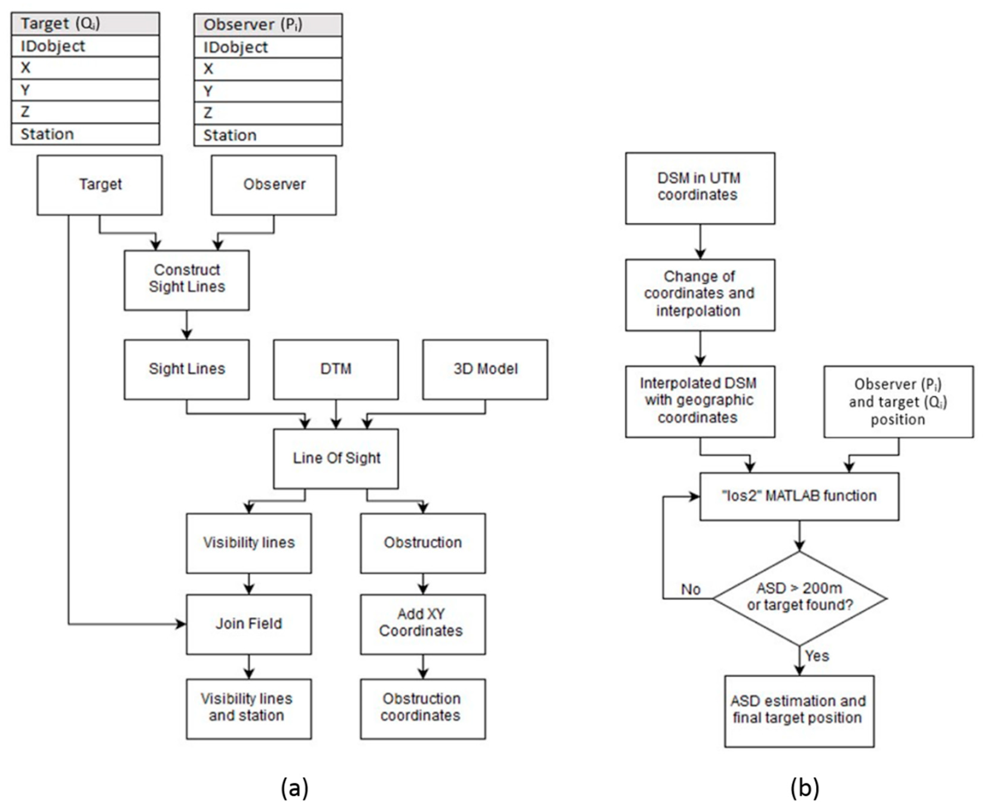
In the GIS platform, the ASD Toolbox was built ad hoc to perform the ASD analysis (Figure 8a). ArcGIS® contains the application ‘Line of Sight’ [11], which analyses and evaluates any intersections with the DTM and the multi patches along a line of sight between two points. However, it only establishes the visibility between one point and many others.
To address this issue, the ASD Toolbox was integrated as a sequence of several geoprocessing tools with the ModelBuilder®, which manages complex workflows replicable through sequences of tools. In ModelBuilder®, the output of the first operation becomes the input of the next one. Instructions are dragged to where the data input and the outputs are required.
In Figure 8a the input data includes: (a) the trajectory of the observer, (b) the position of the target, (c) the DTM, and (d) the multi-patch of all entities that characterize the infrastructure.
The first instruction used in the ASD Toolbox is the ‘Construct Sight Line,’ which connects the observer with all the following targets. The ‘Sight Lines’ are the outputs, which become the input of the ‘Line of Sight.’ The outputs of this second process are (a) the lines of visibility, represented in the screenshot in Figure 7b, which are continuous for the part visible to the observer, and dashed if hidden by an obstruction. Each line of sight is associated with the station of the obstacle it is connected to. The coordinates of the point where the line touches the obstruction constitute the second output of the ‘Line of Sight’ tool. The instruction ‘Add XY Coordinates’ returns the 3D coordinates of such points.
Once the station of the last visible point has been identified, it is subtracted from the station of the observation point and the ASD is then estimated.
The same algorithm was adopted in Matlab® using the instruction named ‘los2,’ which computes the mutual visibility between two points on a DSM [12]. This instruction was included in a proprietary code to manage the trajectories of the observer and the target in the DSM. It automatically generates the ‘line of vision’ between the points and the graph of the surface, and also calculates the coordinates of the obstruction.
Following an initial test, the algorithm was modified to automate the sight analysis in a new coordinate system. In fact, Matlab® requires the position and the DSM model to have geographic coordinates (λ, φ), while the 3D model and trajectories were defined in the WGS84 UTM (Universal Transverse of Mercator) system zone 32N. The new 3D model of the road environment was generated using a dedicated routine, which was specifically developed for this application. The aim was to transform the coordinates, make an interpolation of them, and generate a grid model in a geographic coordinate system [45].
The code in Figure 8b requires input data to start the process, which, in this case, were the DSM and the spreadsheet containing the coordinates of the points forming the trajectories of the observer and the target. The code was designed to allow the user to select data and to immediately execute the coordinate transformation of the trajectory points. An iterative procedure performs the sight analysis for each pair of observer (P) target (Qi) points.
The ASD was estimated by assuming a maximum distance PQi of 200 m, which is greater than the maximum possible values of SSD for vehicles traveling below the speed limits on urban roads. If an obstruction is detected at a distance of less than 200 m, the loop stops and the ASD is calculated as the difference between the station of the last visible target (Qf) and the observation point (P), as in Figure 7a; otherwise, the value of 200 m is assigned to the ASD. This procedure was also adopted to limit the processing time. The loop then restarts and passes to the analysis of the following observation point. At the end of the process, the system automatically generates a new spreadsheet with the ASD results.
Multiple tests on some portions of the model highlighted the potential use of this algorithm for the automatic detection of obstructions. However, conversion of the DSM into geographical coordinates requires a new interpolation as indicated in Section 3.3, which could represent a limit for the analyses, as described in Section 5.
4. Case Study
The case study used for the development of this ASD evaluation methodology consisted of a 500 m stretch of urban arterial road (specifically, Corso Castelfidardo in Turin, Italy) between two at grade signaled intersections (Figure 9). All the 3D images and pictures included in the paper relate to this specific case study. On this road section, the speed limit is 50 km/h. The segment is characterized by an accident frequency rate higher than that observed along sections of the urban road network of Turin.
5. Results and Discussion
The two codes for the ASD analysis were assessed along the section of urban arterial road described in the previous section. The results of the evaluation are presented in Figure 10.
The curvature diagram and the vertical profile of the road section are shown in Figure 10a. The graph testifies to the marked inflection of the stretch between the stations at 200 and 340 m, with a minimum radius of curvature of 50 m. The restrictions to the ASD along this section are due to an almost continuous parking lane on the right margin of the carriageway, and also to some street furniture.
Figure 10b includes a design speed profile that was evaluated from the trajectory curvature as per the Italian road design standard [44], which considers a maximum design speed of 10 km/h above greater that the posted speed limit. On the basis of the standard driver model, the speed is affected by the curvature of the horizontal alignment; speed variations are made at 0.8 m/s2 and occur along transition curves, and eventually possibly on tangents. A spot speed study in dry weather conditions was carried out at on three specific sections to assess whether road geometrics affected the free flow speeds. The 85th percentile of free flow speeds is reported in the same figure.
The comparison between the design and operating speed in Figure 10b demonstrates that, in this case study, operating speeds are not affected by the trajectory curvature and by sight limitations due to the presence of lateral obstructions. Drivers who adopted a certain speed along the straight subsections tended to maintain the same speed in the central part, characterized by a continuous variation of the trajectory curvature, while also employing both lanes in order to reduce the curvature of the trajectory—in particular in free flow conditions such as those encountered for the duration that occurred during the execution of the speed survey.
Figure 10c includes an estimate of the ASD using ArcGIS® with the target set at a height of 10 and then 30 cm, and the SSD estimated as a function of the driver speed behavior as per the Italian standard according to the formula:
where vd is the design speed in m/s, Vd is the design speed in km/h, g is the gravitational acceleration (9.81 m/s2), f is the wheel–road friction, and i is the longitudinal slope of the road (positive for upgrades, negative for downgrades).
A comparison between the SSD and the ASD confirms the limitation in driver visibility in the case of possible emergency stop maneuvers. The comparison between the two solutions obtained for different target heights illustrates the effects of the vertical profile, which presents a significant convexity at the stations 300–400 m (Figure 10a). The graph in Figure 10c confirms that at the station 203 m, the farthest target set at 10 cm above the pavement surface is visible at a distance of 108 m, while when it is set at 30 cm, the driver can see it at a distance of 193 m.
Figure 10d reports the results of the ASD estimated in ArcGIS® and Matlab® with the target height set at 10 cm, and the Matlab® solutions at 15, 20, and 30 cm. The graph shows that as the height increases, the ASD curves estimated with Matlab® tend to rise and get closer to the GIS solution. This is because if the target is placed at a greater height on the pavement, the probability of an intersection between the line of sight and the paved surface decreases, with results that may change in much the same way as was previously discussed for the ArcGIS® solution. Local differences visible around the station at 225 m depend on the different spacing that was adopted for the GIS (around 20 m) and the Matlab® (<1 m) analyses.
Figure 10d highlights the discrepancies between the ArcGIS® and Matlab® solutions, which can be attributed to several factors. The DSM used in this investigation had an accuracy of 15 cm with respect to the 3D model, which is 5 cm greater than the height of the target set at 10 cm. Local irregularities of the paved surface, detectable in Figure 10c between stations 200 and 400 m, also obscured the target point and led to highly variable values of ASD.
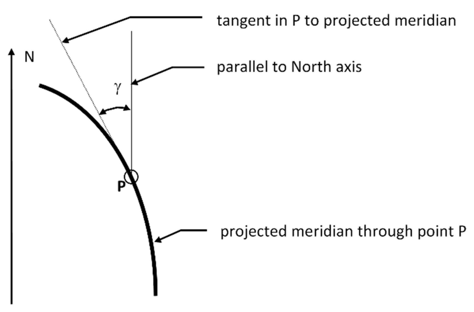
Furthermore, the DSM used in Matlab®, which originated from an interpolation of the GIS model, may present differences and deformations from the first model due to the conversion from projected coordinates of the original 3D model to geographic coordinates, which are illustrated in Figure 11.
As known from literature [46], the mapping grid is rotated with respect to the geographical grid with the angle called meridian convergence (γ), which depends on the position of the point (Figure 11). Moreover, a DSM in cartographic coordinates, with a regular grid with a spatial distribution of 5 cm in East and North, transformed into a DSM in geographic coordinates, does not have regular point distribution. In fact, in the case study, the grid resolution is 0.0025” in longitude and 0.00165” in latitude. This distribution requires a new interpolation of elevations, which leads to a slightly different DSM to that with projected coordinates.
Matlab® can only analyze data belonging to this coordinate system, and the distortion produced by these transformations could have significant effects on modeling results. Furthermore, the two ‘line of sight’ instructions are based on different algorithms that may also generate different surfaces. ArcGIS® uses the Multi-Patch geometry (proprietary format), while Matlab® uses an unknown internal function that cannot be opened or controlled by the operator.
All of the above remarks help to explain the different ASD solutions reported in Figure 10b. It is worth noting once again that small differences between two surfaces and the trajectories of the observer and target may lead to great differences between the two estimates.
According to Table 4, the analysis carried out in the GIS environment takes circa 12 h to investigate just 28 observation points, while the analysis in the numerical computing environment is more efficient, since 776 observation points were processed in less than 1 h.
6. Conclusions
The first part of this research was focused on the analysis of low-cost instruments that would allow the integration of existing models of urban infrastructure with all the elements that could represent an obstruction to visibility. In order to acquire a large number of data in a short time, and to guarantee the repeatability of the acquisitions and the updating of the models, a low-cost MMS system mounted on a vehicle was implemented. The products obtained with these techniques are dense clouds of points that can be further elaborated and used to enrich the already available DSMs. Moreover, the test carried out showed that accuracies appropriate for scale 1:500 and 1:1000 can be reached through these low-cost photogrammetry systems, and the realized products also allow identification of the objects along the roadside, which is an improvement when compared to the current analyses related to the available sight distance (ASD), which are conducted on traditional regional maps (1:10000–25000).
In the second part of the paper, the authors evaluated the performance of software that may be used to investigate the available sight distance (ASD) along stretches of existing roads. A 500 m stretch of a high capacity urban road in Turin (Italy) was used as a case study.
The results indicate that geographic information and numerical computing environments can support sight analyses for road design and road safety investigations. This approach is effective and of interest, since it does not require recourse to in-field direct surveys of the ASD, which involve higher costs, greater risks, and increased data processing time. Moreover, they must be conducted when the roads are traffic free.
Computational and operating differences between the two approaches described in the paper are due to the different accuracy levels of the two investigated models, which also depend on two different coordinate systems. Further investigation is required to understand the reasons behind such differences, in order to eliminate them or compensate for them by taking into account the differences in terms of computational effort, time, and performance.
The investigation is still ongoing, and is principally aimed at simplifying the process of building a reliable DSM, which would reduce the computational effort and limit the differences between the solutions currently available. Although the accuracy of the DSM may not be greater than the height of the obstacle, this approach is, nevertheless, effective in the identification of unsafe road sections. The use of more expensive instruments, like a terrestrial light detection and ranging device (LiDAR), already proposed in [47], could provide a more precise local DSM, which could then be explored with the tools already developed and used in this investigation. This solution is, however, more expensive than those considered here, because it involves the use of geodetic GNSS receivers and high performance IMU sensors.
In any case, one should always bear in mind that the dynamism of urban road space requires the inclusion of appropriate sight obstructions due to moving elements, in contrast to what happens in the rural environment.
Author Contributions
Conceptualization and methodology, M.B. and M.P.; software, validation, and formal analysis, N.G.; investigation, M.B., N.G., M.P. and L.C.; resources, M.B. and M.P.; data curation, N.G. and L.C.; writing, M.B., N.G., M.P. and L.C.; supervision, M.B.; funding acquisition, M.P.
Funding
The investigation described here is part of the Pro VISION Project (funded in 2014 by the Regione Piemonte, Italy).
Acknowledgments
The authors would like to thank the “ICT—Poli di Innovazione Regione Piemonte” and FINPIEMONTE who funded the Pro VISION Project. The other project partners, Beanet s.r.l. and Synarea s.r.l., are also gratefully acknowledged.
Conflicts of Interest
The authors declare no conflict of interest.
References
- AASHTO. Policy on Geometric Design of Highways and Streets, 6th ed.; American Association of State Highway and Transportation Officials: Washington, DC, USA, 2011. [Google Scholar]
- Fitzpatrick, K.; Fambro, D.B.; Stoddard, A.M. Safety Effects of Limited Stopping Sight Distance on Crest Vertical Curves. Transp. Res. Rec. J. Transp. Res. Board 2000, 1701, 17–24. [Google Scholar] [CrossRef]
- Sparks, J.W. The influence of highway characteristics on accident rates. Public Works 1968, 99, 101–103. [Google Scholar]
- Silyanov, V. Comparison of the pattern of accident rates on roads of different countries. Traffic Eng. Control 1973, 14, 432–434. [Google Scholar]
- Urbanik, I.I.; Hinshaw, W.; Fambro, D.B. Safety effects of limited sight distance on crest vertical curves. Transp. Res. Rec. 1989, 1208, 23–35. [Google Scholar]
- Steinauer, B.; Trapp, R.; Böker, E. Verkehrssicherheit in Kurven auf Autobahnen. Straßenverkehrstechnik 2002, 46, 389–393. [Google Scholar]
- Castro, M.; De Santos-Berbel, C. Spatial analysis of geometric design consistency and road sight distance. Int. J. Geogr. Inf. Sci. 2015, 29, 2061–2074. [Google Scholar] [CrossRef]
- Harwood, D.W.; Bauer, K.M. Effect of Stopping Sight Distance on Crashes at Crest Vertical Curves on Rural Two-lane Highways. Transp. Res. Rec. J. Transp. Res. Board 2015, 2486, 45–53. [Google Scholar] [CrossRef]
- Nehate, G.; Rys, M. 3D calculation of stopping-sight distance from GPS data. J. Transp. Eng. 2006, 132, 691–698. [Google Scholar] [CrossRef]
- Ismail, K.; Sayed, T. New algorithm for calculating 3D available sight distance. J. Transp. Eng. 2007, 133, 572–581. [Google Scholar] [CrossRef]
- Environmental Systems Research Institute. ArcObjects Library Reference. 2015. Available online: http://desktop.arcgis.com/en/arcmap/10.3/tools/3d-analyst-toolbox/line-of-sight.htm (accessed on 13 December 2018).
- MathWorks. MATLAB User Manual; MathWorks: Natik, MA, USA, 2011. [Google Scholar]
- Khattak, A.J.; Shamayleh, H. Highway Safety Assessment through Geographic Information System-Based Data Visualization. J. Comput. Civ. Eng. 2005, 19, 407–411. [Google Scholar] [CrossRef]
- Castro, M.; Iglesias, L.; Sánchez, J.A.; Ambrosio, L. Sight distance analysis of highways using GIS tools. Transp. Res. Part C Emerg. Technol. 2011, 19, 997–1005. [Google Scholar] [CrossRef]
- Castro, M.; Anta, J.A.; Iglesias, L.; Sánchez, J.A. GIS-Based System for Sight Distance Analysis of Highways. J. Comput. Civ. Eng. 2014, 28, 04014005. [Google Scholar] [CrossRef]
- Hartley, R.; Zisserman, A. Multiple View Geometry in Computer Vision; Cambridge University Press: Cambridge, UK, 2003. [Google Scholar]
- Remondino, F.; El-Hakim, S. Image-based 3D modelling: A review. Photogramm. Rec. 2006, 21, 269–291. [Google Scholar] [CrossRef]
- Goesele, M.; Curless, B.; Seitz, S.M. Multi-view stereo revisited. In Proceedings of the 2006 IEEE Computer Society Conference on Computer Vision and Pattern Recognition (CVPR’06), New York, NY, USA, 17–22 June 2006; pp. 2402–2409. [Google Scholar]
- Remondino, F.; Spera, M.G.; Nocerino, E.; Menna, F.; Nex, F. State of the art in high density image matching. Photogramm. Rec. 2014, 29, 144–166. [Google Scholar] [CrossRef]
- Haala, N.; Rothermel, M. Image-based 3D data capture in urban scenarios. In Photogrammetric Week ‘15; Wichmann/VDE Verlag: Berlin/Offenbach, Germany, 2015; pp. 119–130. [Google Scholar]
- AASHTO. Highway Safety Manual, 1st ed.; American Association of State Highway and Transportation Officials: Washington, DC, USA, 2010. [Google Scholar]
- Liu, L.; Zhang, L.; Ma, J.; Zhang, L.; Zhang, X.; Xiao, Z.; Yang, L. An improved line-of-sight method for visibility analysis in 3D complex landscapes. Sci. China Inf. Sci. 2010, 53, 2185–2194. [Google Scholar] [CrossRef]
- Alsadik, B.; Gerke, M.; Vosselman, G. Visibility analysis of point cloud in close range photogrammetry. ISPRS Ann. Photogramm. Remote Sens. Spat. Inf. Sci. 2014, 2. [Google Scholar] [CrossRef]
- Peters, R.; Ledoux, H.; Biljecki, F. Visibility analysis in a point cloud based on the medial axis transform. In Proceedings of the Eurographics Workshop on Urban Data Modelling and Visualisation, Delft, The Netherlands, 23 November 2015; pp. 7–12. [Google Scholar]
- González-Jorge, H.; Díaz-Vilariño, L.; Lorenzo, H.; Arias, P. Evaluation of driver visibility from mobile lidar data and weather conditions. Int. Arch. Photogramm. Remote Sens. Spat. Inf. Sci. 2016, 41. [Google Scholar] [CrossRef]
- U.S. Department of Transportation, Federal Highway Administration. Visual Impact Assessment for Highway Projects; U.S. Department of Transportation, Federal Highway Administration: Washington, DC, USA, 1990.
- Bartie, P.; Reitsma, F.; Kingham, S.; Mills, S. Advancing visibility modelling algorithms for urban environments. Comput. Environ. Urban Syst. 2010, 34, 518–531. [Google Scholar] [CrossRef]
- Delikostidis, I.; Engel, J.; Retsios, B.; van Elzakker, C.P.J.M.; Kraak, M.J.; Döllner, J. Increasing the usability of pedestrian navigation interfaces by means of Landmark visibility analysis. J. Navig. 2013, 66, 523–537. [Google Scholar] [CrossRef]
- Available online: http://desktop.arcgis.com/en/documentation/ (accessed on 2 January 2019).
- Available online: http://www.skylineglobe.com/SkylineGlobe/corporate/default.aspx (accessed on 2 January 2019).
- Tandy, C.R.V. The isovist method of landscape survey. In Methods of Landscape Analysis; Landscape Research Group: London, UK, 1967; pp. 9–10. [Google Scholar]
- Benedikt, M.L. To take hold of space: Isovists and isovist fields. Environ. Plan. B Plan. Des. 1979, 6, 47–65. [Google Scholar] [CrossRef]
- Turner, A.; Doxa, M.; O’sullivan, D.; Penn, A. From isovists to visibility graphs: A methodology for the analysis of architectural space. Environ. Plan. B Plan. Des. 2001, 28, 103–121. [Google Scholar] [CrossRef]
- Van Bilsen, A. Mathematical Explorations in Urban and Regional Design. Ph.D. Thesis, Delft University of Technology, Delft, The Netherlands, 2008. [Google Scholar]
- Piras, M.; Cina, A.; Lingua, A. Low cost mobile mapping systems: An Italian experience. In Proceedings of the 2008 IEEE/ION Position, Location and Navigation Symposium, Monterey, CA, USA, 5–8 May 2008; pp. 1033–1045. [Google Scholar]
- Schwarz, K.P.; El-Sheimy, N. Mobile mapping systems–state of the art and future trends. Int. Arch. Photogramm. Remote Sens. Spat. Inf. Sci. 2004, 35 Pt B, 10. [Google Scholar]
- Haala, N.; Peter, M.; Cefalu, A.; Kremer, J. Mobile lidar mapping for urban data capture. In Proceedings of the 14th International Conference on Virtual Systems and Multimedia, Limassol, Cyprus, 20–25 October 2008; Volume 2025, p. 95100. [Google Scholar]
- Anguelov, D.; Dulong, C.; Filip, D.; Frueh, C.; Lafon, S.; Lyon, R.; Weaver, J. Google street view: Capturing the world at street level. Computer 2010, 43, 32–38. [Google Scholar] [CrossRef]
- Kukko, A.; Kaartinen, H.; Hyyppä, J.; Chen, Y. Multiplatform mobile laser scanning: Usability and performance. Sensors 2012, 12, 11712–11733. [Google Scholar] [CrossRef]
- Papadopoulos, G.; Kurniawati, H.; Shariff, A.S.B.M.; Wong, L.J.; Patrikalakis, N.M. 3D-surface reconstruction for partially submerged marine structures using an Autonomous Surface Vehicle. In Proceedings of the 2011 IEEE/RSJ International Conference on Intelligent Robots and Systems, San Francisco, CA, USA, 25–30 September 2011; pp. 3551–3557. [Google Scholar]
- McGlone, J.C.; Mikhail, E.; Bethel, J. Manual of Photogrammetry, 5th ed.; American Society for Photogrammetry and Remote Sensing: Bethesda, MD, USA, 2004. [Google Scholar]
- Aicardi, I.; Lingua, A.; Piras, M. Evaluation of Mass Market Devices for the Documentation of the Cultural Heritage. Int. Arch. Photogramm. Remote Sens. Spat. Inf. Sci. 2014, XL, 17–22. [Google Scholar] [CrossRef]
- Snavely, N.; Seitz, S.M.; Szeliski, R. Photo tourism: exploring photo collections in 3D. ACM Trans. Graph. 2006, 25, 835–846. [Google Scholar] [CrossRef]
- Ministero delle Infrastrutture e dei Trasporti. Norme Funzionali e Geometriche per la Costruzione delle Strade; Decreto Ministeriale No. 6792; Italian Ministry of Transportation Decreto Ministeriale: Roma, Italy, 2001. (In Italian)
- Soler, T.; Hothem, L.D. Coordinate Systems Used in Geodesy: Basic Definitions and Concepts. J. Surv. Eng. 1988, 114, 84–97. [Google Scholar] [CrossRef] [Green Version]
- Bugayevskiy, L.M.; Snyder, J. Map Projections: A Reference Manual; CRC Press: Boca Raton, FL, USA, 1995. [Google Scholar]
- Tsai, Y.; Yang, Q.; Wu, Y. Use of Light Detection and Ranging Data to Identify and Quantify Intersection Obstruction and Its Severity. Transp. Res. Rec. J. Transp. Res. Board 2011, 2241, 99–108. [Google Scholar] [CrossRef]
Figure 1.
Conceptual relationship between available sight distance (ASD) and crash rate (adapted from [2]).
Figure 1.
Conceptual relationship between available sight distance (ASD) and crash rate (adapted from [2]).

Figure 2.
Estimation of the ASD along a road section with sight obstructions of different heights.

Figure 3.
Workflow for the digital surface model (DSM) generation: (a) orthophoto of Turin and 2D geographic information system (GIS) of the road infrastructure; (b) 3D model of the urban environment, floating on the DTM; (c) elevation model built from the 3D model, the original digital terrain model (DTM) resampled and cut in relation to the 3D model, and the DSM.

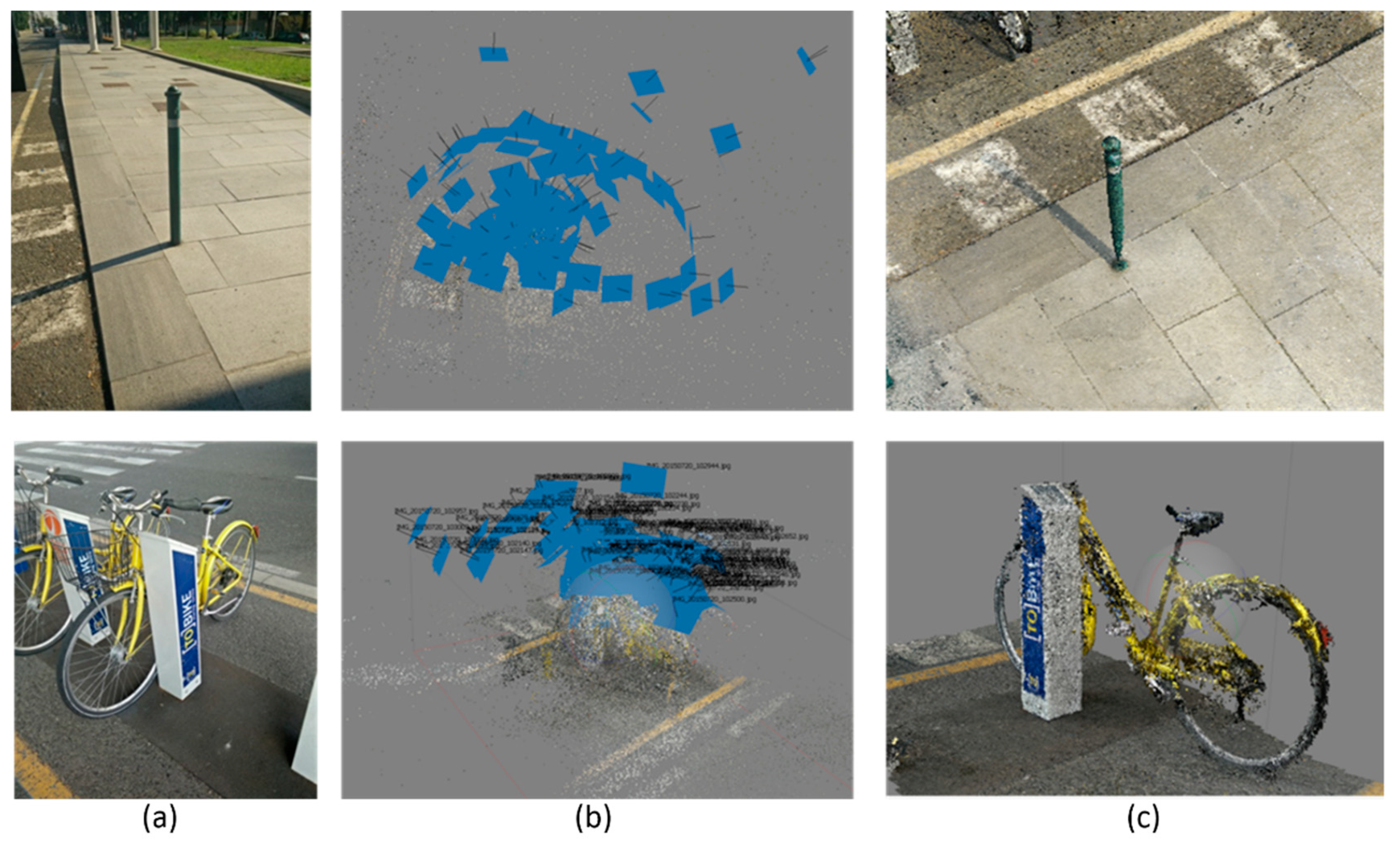
Figure 4.
3D object reconstruction by structure from motion (SfM), applied along the road section of the case study. (a) Street furniture was first photographed from different angles with a smartphone; (b) the software relocates the images to the correct spatial location and extracts a 3D point cloud; (c) the cloud is densified and points are used to build the 3D surface of objects.

Figure 5.
The resulting geo-referenced dense point cloud of the road infrastructure (on the right) and the detail of the parked cars.
Figure 5.
The resulting geo-referenced dense point cloud of the road infrastructure (on the right) and the detail of the parked cars.

Figure 6.
The image captured from the MMS vehicle (on the left) and the updated 3D model reconstructed on the ArcGIS platform (on the right), comprising all the elements existing in the urban infrastructure.
Figure 6.
The image captured from the MMS vehicle (on the left) and the updated 3D model reconstructed on the ArcGIS platform (on the right), comprising all the elements existing in the urban infrastructure.

Figure 7.
(a) Horizontal and vertical 2D and (b) 3D representation of the algorithm used for estimating the ASD (the continuous line represents the visible part of the line of sight, while the dashed one is the portion blinded by the sight obstruction).
Figure 7.
(a) Horizontal and vertical 2D and (b) 3D representation of the algorithm used for estimating the ASD (the continuous line represents the visible part of the line of sight, while the dashed one is the portion blinded by the sight obstruction).

Figure 8.
(a) Workflow of the ASD Toolbox built with ModelBuilder®; (b) workflow of the ASD tool in the numerical computing environment.
Figure 8.
(a) Workflow of the ASD Toolbox built with ModelBuilder®; (b) workflow of the ASD tool in the numerical computing environment.

Figure 9.
Maps with geographic and cartographic coordinates of the two extremes of the road section investigated as a case study.
Figure 9.
Maps with geographic and cartographic coordinates of the two extremes of the road section investigated as a case study.

Figure 10.
(a) Vertical profile and trajectory curvature; (b) design speed profile and operating speed values; (c) comparison between stopping sight distance (SSD) and ASD, estimated at 10 cm and 30 cm in accordance with the ArcGIS® code; (d) comparison between ASD estimated with ArcGIS® and Matlab® at 10 cm, and the variation in Matlab® solutions at 15, 20, and 30 cm.

Figure 11.
Convergence of a meridian (angle—γ—formed by the representation of the meridian with the north of the projection—i.e., vertical axis of the Cartesian reference system).
Figure 11.
Convergence of a meridian (angle—γ—formed by the representation of the meridian with the north of the projection—i.e., vertical axis of the Cartesian reference system).


Table 1.
Characteristics of the personal computer employed for data processing.
| Characteristics | Personal Computer |
|---|---|
| Operating system | Windows 7 Professional x64 |
| Processor | Intel® Core™ i7-5600U with Intel HD Graphics 5500 |
| Memory capacity | 16 GB DDR3L-1600 SDRAM |
| Flash cache | 32 GB M.2 |
Table 2.
Smartphone specifications.
| Characteristics | OnePlus One |
|---|---|
| Operating System | Android 5.1.1 |
| Cost (€) | 215 |
| Camera type | CMOS |
| Camera model | 13MP Sony Exmor RS IMX 214 F2.0 |
| Max image resolution (pixel) | 4128 × 3096 |
| Dimension (mm) | 154.2 × 74.1 × 7.25 |
Table 3.
Sensors and devices installed on the mobile mapping system (MMS).
| Position of devices installed on the bar |  | ||
| Sensor | Image | Cost | Data acquired and storage |
| A: Ublox EVK 6T: GPS receiver single Frequency (L1) |  | ≈400 € | GPS raw data and PVT (position velocity and timing) solution in real time. Acquisition by laptop |
| B: Garmin VIRB Elite |  | ≈250 € | Images (16Mpx@CMOS sensors) and Video (Full HD). GPS integrated for tracking and frame geo-referencing. Internal memory |
| C: Webcam Logitech 920C |  | ≈100 € | Images (15MPx@CMOS sensors) and videos (full HD). Carl Zeiss optical lens for high quality frames. No internal GPS. Acquisition by laptop |
| D: Microstrain 3DM-GX3-35 Inertial platform (IMU) |  | ≈3500 € | Acceleration and angular velocity. Attitude and position. GPS time synchronized. Acquisition by laptop |
Table 4.
Comparison of ArcGIS® and Matlab® solutions.
| Software | ArcGIS®—ASD Toolbox | Matlab® |
|---|---|---|
| Reference system | UTM | Latitude and longitude |
| Number of observation points | 28 | 776 |
| Length of the road section | 500 m | 500 m |
| Computational time (with the personal computer described in Table 1) | 12 h in total, during which time the presence of the operator was required to relaunch the calculation at each observation point | <1 h (fully automated process) |
© 2019 by the authors. Licensee MDPI, Basel, Switzerland. This article is an open access article distributed under the terms and conditions of the Creative Commons Attribution (CC BY) license (http://creativecommons.org/licenses/by/4.0/).
Share and Cite
MDPI and ACS Style
Bassani, M.; Grasso, N.; Piras, M.; Catani, L. Estimating the Available Sight Distance in the Urban Environment by GIS and Numerical Computing Codes. ISPRS Int. J. Geo-Inf. 2019, 8, 69. https://doi.org/10.3390/ijgi8020069
AMA Style
Bassani M, Grasso N, Piras M, Catani L. Estimating the Available Sight Distance in the Urban Environment by GIS and Numerical Computing Codes. ISPRS International Journal of Geo-Information. 2019; 8(2):69. https://doi.org/10.3390/ijgi8020069
Chicago/Turabian StyleBassani, Marco, Nives Grasso, Marco Piras, and Lorenzo Catani. 2019. "Estimating the Available Sight Distance in the Urban Environment by GIS and Numerical Computing Codes" ISPRS International Journal of Geo-Information 8, no. 2: 69. https://doi.org/10.3390/ijgi8020069
Note that from the first issue of 2016, this journal uses article numbers instead of page numbers. See further details here.