Abstract
Identifying group movement patterns of crowds and understanding group behaviors are valuable for urban planners, especially when the groups are special such as tourist groups. In this paper, we present a framework to discover tourist groups and investigate the tourist behaviors using mobile phone call detail records (CDRs). Unlike GPS data, CDRs are relatively poor in spatial resolution with low sampling rates, which makes it a big challenge to identify group members from thousands of tourists. Moreover, since touristic trips are not on a regular basis, no historical data of the specific group can be used to reduce the uncertainty of trajectories. To address such challenges, we propose a method called group movement pattern mining based on similarity (GMPMS) to discover tourist groups. To avoid large amounts of trajectory similarity measurements, snapshots of the trajectories are firstly generated to extract candidate groups containing co-occurring tourists. Then, considering that different groups may follow the same itineraries, additional traveling behavioral features are defined to identify the group members. Finally, with Hainan province as an example, we provide a number of interesting insights of travel behaviors of group tours as well as individual tours, which will be helpful for tourism planning and management.
1. Introduction
With the progress of location-acquisition techniques, a large amount of spatio-temporal data can be acquired from GPS, Wi-Fi, cellular networks and Location-Based Social Networks(LBSN) in the form of trajectories. The increasing trajectory data enables us to discover knowledge that is meaningful in aiding the research of human mobility. A branch of research aimed at discovering group movement patterns in order to analyze behaviors of group members has attracted attentions in recent years [1,2,3,4,5,6,7,8,9,10]. Some group movement patterns have been proposed in previous studies like flock [3], convoy [4], swarm [5], traveling companion [6,7,8] and gathering [9], which are summarized in [10]. Identifying object groups that move together for a certain period of time can benefit various applications. For example, commuters can discover people with the same route for car sharing. Scientists could get deep understanding of the migration patterns of animals. These patterns consider the number of the snapshots corresponding to the time when the objects stay together as the measurement to judge whether they constitute a group. Usually, these patterns perform well on high-quality GPS data. But for some trajectory data with low spatial resolution and sampling rate, these patterns may not be discovered correctly.
In this paper, we put efforts into discovering groups of tourists who travel together for a certain time period using anonymized Call Detail Records (CDRs) data. The travel behaviors of group members are then explored, which are of great value to the research of tourism. For example, travel itineraries can be designed more specifically according to the different travel behaviors of group tourists and individual tourists. CDR data contains time and location information of mobile phone users corresponding to when and where the records were generated. Compared to GPS data, CDR data can be obtained at a lower cost and on a scale of millions of users easily. So CDRs are useful in trajectory data mining and human mobility analysis at a city level.
However, we are still facing some challenges in the process of mining tourist group movement patterns from the huge amount of CDR data. Firstly, it can be very time-consuming if we try to discover groups from the trajectory data which consists of thousands or even millions of users. The second challenge comes from the sparsity in both spatial and temporal resolutions of CDR data. Despite the huge scale of the trajectory data acquired from CDRs, the data of every single user is of low accuracy and frequency. So the traditional similarity metrics for GPS trajectories are not applicable to CDR data. The third challenge is the complexity of tourists behaviors. Generally, tourists are willing to visit well-known scenic areas. When different groups visit the same scenic areas, their trajectories may overlap, which makes it hard to distinguish between two groups with similar travel routes. Besides, group members may not travel together all the time, some members who are more active may have a larger range of activities. In such a situation, if we discover groups only by the number of the timestamps when the objects stay together, the result will be imprecise. Therefore, other features need to be considered to help identify different tourist groups.
Considering the challenges we are facing, we propose a Group Movement Pattern Mining based on Similarity (GMPMS) to identify co-movement patterns from low accuracy trajectory data. Unlike the moving together patterns summarized in [10], GMPMS disregards the restrictions on the shape or density of a group. Instead, trajectory similarity and some other features such as accommodation similarity are used to capture the group movement patterns from sparse trajectories.
We first remove massive trajectories of objects who are impossible within a group and get candidate groups by employing the frequent item set mining method. In this step, only tourists that stay together within a predefined distance during a certain period are retained as candidate groups. Next, we design a method to measure the similarity of tourists in each candidate group considering multiple features extracted from the trajectory data, such as trajectory similarity, accommodation similarity and other traveling features that can reflect the relationship between the group members. Finally, a semi-supervised learning algorithm is used to identify real tourist groups from the candidate groups.
The main contributions presented in this paper are:
- We proposed a new group movement pattern mining method based on similarity that can identify groups from a huge amount of mobile trajectory data;
- We designed an algorithm to calculate trajectory similarity of objects with low accuracy data;
- We explored different travel behaviors of group and individual tourists.
The rest of the paper is organized as follows: Section 2 discusses related work. Section 3 describes the problem in this work and the overall algorithms for mining tourist group movement patterns. Section 4 shows our experimental study, and Section 5 discusses the results. The paper closes with the conclusions in Section 6.
2. Related Works
2.1. Group Movement Mining
Discovering groups of the objects that move together for a certain period is an important research objective in mobility studies. Some inferences have been proposed to explain different group patterns. These group patterns can be distinguished from three aspects: the shape of the groups, whether the groups are continuous, and whether the members are variable during the lifespan of the pattern [1].
The flock [3] pattern is a group of objects that travel together within a circle of some user-specified size for at least K consecutive timestamps. And recently, Sanches, D.E. et al. [11] introduced the concept of k-co-movement patterns and proposed a top-down algorithm with free distance parameter to improve the flock pattern. However, the group in flock is restricted in a circular region that will lead to a lossy-flock problem. To solve the problem, the convoy [4,12] pattern is proposed to describe arbitrary shape of groups by using density-based clustering. Li et al. proposed swarm [5], which allows the K timestamps not to be consecutive. Because of the fact that the members of a group are not always gathered, this pattern allows the members to disappear for some time as long as they stay together for at least K timestamps. Tang et al. [8] proposed a traveling companion pattern, which uses a data structure called traveling buddy to continuously find patterns. This pattern can be regarded as an online detection fashion of convoy.
Besides, Zheng et al. [9] proposed a gathering pattern to discover various group incidents such as celebrations, parades and so on. Wang et al. [13] proposed two kinds of loose group movement patterns namely Weakly Consistent Group Movement Pattern (WCGMP) and Weakly Consistent and Continuous Group Movement Pattern (WCCGMP), and corresponding discovery algorithms. The WCGMP and the WCCGMP are collectively referred to as the loose group movement patterns, in which the gatherings of a group could be partial and variable during the group’s lifespan. Zhang et al. [14] proposed the GMOVE pattern and adopted HMMs to build a model. And recently, Phan, N. et al. [15] redefined the movement patterns and proposed a unifying approach, GeT_Move, which used a frequent closed itemset-based pattern mining algorithm to optimize the processing efficiency. And Lee, J.G. et al. [16] considered mining the trajectory patterns of various temporal tightness to cover all the trajectory patterns.
Patterns mentioned above can be used to find co-travelers. But due to the low accuracy of CDRs and the complexity of travel behaviors, these patterns may be not suitable in our study. The reason is discussed in the Section 3.
2.2. Trajectory Similarity
Devices that can be used to track moving objects have increased dramatically, leading to a great growth in movement data. Most movement data is captured and stored in the form of trajectories. One important class of trajectory analysis is the measurement of similarity between trajectories. Several similarity metrics have been proposed to calculate the distance between two trajectories, such as Longest Common Subsequence (LCSS) [17,18], Dynamic Time Warping (DTW) [19], Edit Distance (ED) [20,21,22] and so on [23,24].
DTW searches all point combinations between two trajectories for the one with minimal cost even if they are not aligned in the time axis. So the similarity between trajectories of different lengths and with local time shifting can be computed. LCSS can be used as a similarity measure in which some points are able to remain unmatched in an attempt to provide an accurate similarity result. However, for trajectories with widely varying sampling rates, it may lead to many points being unmatched. ED is to count the minimum number of edits required to make two trajectories equivalent. Several variations of edit distance exist, including Edit Distance with Real Penalty (ERP) [20] and Edit Distance on Real Sequence (EDR) [21]. ERP and EDR both take into account local time shifting and allow similarities to be found between trajectories of different lengths.
Besides, a shape-based similarity measure for trajectory data is proposed by [25], which is based on vectors instead of individual data points. Liu, H. et al. [26] also focused on measuring similarity between moving objects, and defined the trajectory similarity from the geographic and semantic aspect. In addition, Wang, F. et al. [27] designed a novel semantic trajectory similarity measure to estimate similarity among users. Ra, M. et al. [28] proposed an effective trajectory similarity measure that incorporated the geographic and semantic similarities simultaneously.
However, in our work, the trajectory data extracted from CDRs is of low accuracy. Similarity measures mentioned above are not suitable because we need to deal with the influence caused by different sampling rates and data sparsity. The algorithms that go through all points to compare each pair of points to detect similarity may be not precise. In this case, a novel algorithm to measure trajectory similarity in low accuracy is needed.
2.3. Travel Behaviors
To get an insight of travel behaviors, many researchers make efforts to mine tourist behavior patterns using GPS data from mobile devices, check-ins collected from social network, geo-tagged photos uploaded by tourists, GIS information and so on. Xue, M. et al. [29] identified the tourists among public commuters using the public transportation data provided by Singapore’s Land Transport Authority and then revealed the traveling patterns of tourists. Vu H.Q. et al. [30] looked insights into tourist behaviors by exploiting the socially generated and user-contributed geotagged photos that have been made publicly available on the Internet. And similarly, Yang, L. et al. [31] and Onder, I. et al. [32] utilized geo-tagged photos from Flickr to extract trajectories of tourists to detect tourist mobility patterns. In addition, the Twitter and Foursquare data were also widely used in the travel behaviors analysis. For example, Maeda, T. et al. [33,34] extracted the different preferences of tourists from different countries by characterizing each location. And Sun, Y. et al. [35] empirically investigated the travel and activity patterns of active local Foursquare users in New York City. Besides the social media data mentioned above, Phithakkitnukoon, S. et al. [36] also analyzed tourist behaviors in Japan using massive mobile phone GPS location records. Barkhordari, R. et al. [37] examined the motivations of different tourists with the true visiting records of National Park in Malaysia.
Despite much effort putting into travel behaviors mining, to have a full understanding of tourist behaviors in an area is still not an easy task. One of the most important reason is that different kinds of tourists may have different behaviors, which leads to the diversity of travel behaviors. In our work, we try to analyze travel behaviors and find out the difference between group tourists and individual tourists.
2.4. Application of Group-Level Analysis
The group identification and analysis are valuable in many fields, such as the human mobility modeling, group feature mining and relationship recognition. And recently, many researchers have put their efforts into the group-level analysis to address the sparsity and complexity of individual modeling.
Specifically, Zhang, C. et al. [14] proposed GMOVE, a group-level mobility modeling method to obtain quality mobility models from the highly sparse and complex GeoSM data. Their insight was that the users within the same group may share significant movement regularity. And Caughey, D. et al. [38] developed a Bayesian group-level IRT approach that models latent traits at the level of demographic and/or geographic groups rather than individuals, and thus the political opinions could be obtained by sufficient polls in each group. And similarly, Bos, E.H. et al. [39] utilized the identified groups to mine the overall features of different categories and made classifications for the whole population. In addition, group-based analysis was also widely utilized in medical applications [40,41] to get categories and achieved accurate modeling of the patients. And during the recent years, the analysis of intra-group interactions also received much attention. For example, Moore-Russo, D. et al. [42] investigated a Facebook group on the interactions among students, alumni and faculty, which can support and recognize social connections among group users.
3. Materials and Methods
In this section, we first introduce the data set we used in this research. The problem and framework of group pattern mining is presented then. We also described the proposed group movement pattern mining based on similarity method in detail.
3.1. Problems and Framework
To identify tourist groups based on the trajectories of individuals is to discover traveling companions for the entire trips. The method we proposed to find out groups from all tourists takes into account similarity between tourists and is designed for low accuracy CDR data. The framework of our project will also be shown in this section.
3.1.1. Problem Definition
In the field of group pattern mining, some common concepts are shared in many different studies. In this section, we employ some notations of trajectory mining, and then illustrate the problem we aim to solve. The notations used throughout this paper are listed in Table 1.

Table 1.
Description of the Notations.
In this paper, two types of cellular data are used. One is CDR which is generated when there are incoming or outgoing calls or short messages. The other is location-based data generated in the case of some passive network events, such as when hand over happens between two adjacent cells, or after half an hour of inactivity of the mobile phone. For the sake of simplicity, we refer these two types of data as CDRs. The coverage radius of the base stations varies from 500 to 2000 m. CDRs provide a compromise between spatio-temporal resolution and ubiquity. As shown in Table 2, each record in the raw CDR data set contains an anonymous user id, the timestamp of the record, the location id which represented by the base station id to which the user connected, the latitude and longitude of the base station, and the user’s home location which discloses from which province the user comes. To discover the patterns of group movement, we need to identity the stay points which usually stand for a meaningful location and convert the raw dataset to a sequence of trajectories which separated by the stay points. Group members may have the same stay points where they gather together for a certain period.
Table 2.
Data format of Call Detail Records (CDRs).
Problem Statement: Given a trajectory set of moving object set and similarity threshold , our task is to discover all the groups in which the movement similarity of the members is greater than .
Compared to GPS trajectories, trajectories generated from CDR data set have much lower spatial and temporal resolution. In Figure 1, we plot the cumulative distribution function and normalized histogram of the distance and time interval between two adjacent records. There are more than 95% records for which the distance between the trajectory points determined by the adjacent records is greater than 200. The peak at 500 m shows that the coverage radius of most base stations is 500 m. About 60% records have the time interval between the adjacent records greater than 1000 s. There is a sudden increase in the position of around 1800 s, which indicates the location updates within half an hour. In addition to the poor resolution in space and time, inconsistent and non-uniform sampling rates of the trajectories which is inherently the problem for CDR data have to be tackled in particular. Even if two tourists traveled together for the whole journey, the number of their trajectory points may vary greatly and their trajectory points are not aligned with each other. In an extreme case, the trajectory points of the two tourists traveling together may be recorded at alternating times. So it is necessary to design an algorithm to deal with these issues of the CDR trajectory data.
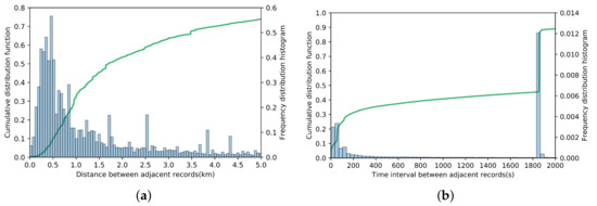
Figure 1.
Distribution of the distance and time interval between adjacent records. (a) Distribution of the distance between adjacent records; (b) Distribution of the time interval between adjacent records.
As shown in Figure 2, the trajectories of four objects are divided into seven snapshots. Each snapshot contains the trajectory points of users within a predefined period time. Considering the missing data, we use points with “x” label to indicate the locations that are missed in the dataset. In each snapshots, the objects within a distance limit are gathered into clusters. The parameter M denotes the minimum number of members in a group and K denotes the minimum number of snapshots for the occurrence of groups. As shown in Figure 2, where M is 2 and K is 3, the flock and the convoy pattern require at least K consecutive snapshots. So the group and can be discovered by both flock and convoy. The swarm pattern is not restricted to the consecutiveness, so it can get more groups as .
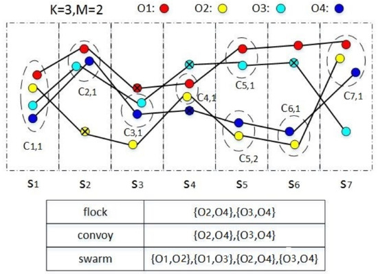
Figure 2.
Group movement patterns. The results of different patterns are exhibited in the table.
However, it can be seen that is also a group, but this group can’t be identified because is missed in and are missed in .
Besides the sparsity of CDRs, there is another abnormal situation when identifying these moving together patterns. In Figure 2, when K is set to be 3, is identified as a swarm pattern. However, it is obvious from the figure that and stay together only in , and . The trajectory of the two objects is not similar in other four snapshots. Moreover, we can’t filter out this kind of groups by increasing the value of K. Because when K is set to be 4, the real group can’t be identified from snapshots. In such a case, it is hard to choose the value of K when identifying groups. Hence a new method need to be proposed to solve this problem.
So in this paper, we proposed a method called Group Movement Pattern Mining based on Similarity (GMPMS) to solve this problem by calculating the similarity between objects from multiple dimensions and is able to identify tourist groups from sparse CDR data.
3.1.2. Framework
In this part, we will introduce the framework of discovering the group movement patterns based on similarity. We are interested in not only discovering co-movement patterns but also analyzing travel behaviors of different groups of tourists. Figure 3 exhibits our framework diagram. The left column shows data sources, including call record details, points of interest of scenic areas and map data. The column in the middle shows the key components of our algorithm. After data preprocessing and candidate groups filtering, similarity between any two trajectories in each candidate group is computed to obtain the possible co-movement pairs. Then groups are identified based on a semi-supervised learning algorithm or a threshold-based method. Finally, travel behaviors of group and individual tourists are analyzed to get some insights of the tourists. The right column shows the output of our framework.
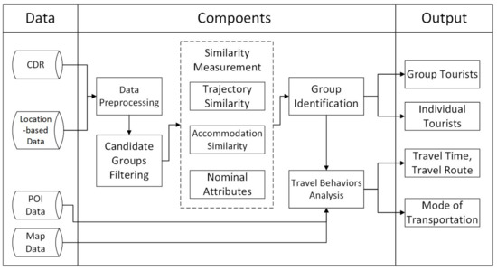
Figure 3.
Modeling framework diagram.
3.2. Data Preprocessing
In this paper, we focus on the travel behaviors analysis of group tourists and individual tourists in Hainan province. At the foremost, we need to extract the trajectories of the tourists. Tourists identification is non-trivial though, we simplified the problem by an assumption that the tourists are those whose mobile phone’s home location are provinces other than Hainan. In CDR data, there is one field that indicates which province the user belongs to. So we remove the users with this field indicating Hainan at first. The remaining users are regarded as tourists. Besides, we also discard the trajectory data of the users whose total number of records is less than 100 per month, which may not contribute to the analysis.
When a mobile phone is in the overlapped areas between adjacent cells, it may switch between two cells when actually the user’s location hasn’t changed. This phenomenon is called the Ping-pong effect which leads to abnormal trajectory in the data. To eliminate such noise, we refer to [43] for detecting and removing oscillation records. After that, we identify stay points from raw trajectories.
Definition 1.
(Stay Point): A stay point represents a location characterized by a sequence of consecutive points in the raw trajectory data which is limited by both temporal and spatial constraints.
For a given trajectory , a stay point is defined as the centroid of a sub-trajectory , , which satisfies the condition that distance between two points in is less than a threshold , the time interval between and is greater than a threshold .
A stay point is generated from and can be denoted as , where u is the id of the user, x and y are the longitude and latitude of the centroid of , t is the timestamp of the first point of i.e., , and is the time interval between and in , which indicates how long a user stays in this region.
After identifying stay points from raw data, the trajectory of a user converts into a sequence of pass-by points separated by some stay points. The points which do not satisfy the conditions in Definition 1 are called pass-by points.
3.3. Candidate Groups Filtering
After data preprocessing, we are able to calculate the similarity between tourists to identify tourist groups with high similarity between its members. A group of tourists traveling together must have some features in common, such as trajectory, accommodation and so on. Our algorithm aims to discover tourist groups whose members have similar behaviors in relation to each other. However, too many tourists means that the process of similarity calculation between all pairs of tourists will be overwhelmingly time-consuming as well as memory consuming. To solve the problem, we filter out massive trajectories of tourists who are impossible within a tourist group at first by deploying a frequent itemset mining method before the process of similarity measurement. In this step, we can get candidate groups whose members appeared together for at least K snapshots of the trajectories. So only the similarity among tourists in a candidate group rather than all tourists need to be computed, which greatly reduces the computational complexity.
Considering that the stay points of the members in one tourist group should be close to each other in space for most of the time, we can remove the trajectories of tourists who don’t satisfy these conditions and may be individual tourists by applying a frequent itemsets mining method.
At first, we divide a trajectory into a sequence of snapshots by time. Let be the interval of snapshots, be the time span of the considered group movement patterns. Snapshot set S is a sequence of snapshots , . Each element can be expressed as a set of stay points in trajectory, i.e., , where is the start time of the i-th snapshot, is the j-th stay point whose timestamp is within the interval of the snapshot i and n is the total number of stay points in the snapshot.
For the sake of the sparsity data of CDRs and its inconsistent sampling rate of trajectories, the interval of snapshots need to be selected long enough to ensure that the trajectory points can be included in the same snapshots as long as the difference of their timestamps is no more than .
Definition 2.
(Collection): A collection c is a group of stay points in a snapshot within a distance threshold . The snapshot can be expressed in collections as , where is the j-th collection in and m is the total number of collections in .
For example, as shown in Figure 2, to denote seven continuous snapshots, each of which contains stay points whose timestamp is within the interval of the snapshot. And the objects in a snapshot within a distance threshold belong to a collection. A snapshot may contain numbers of collections. As in , there are two collections and . In this work, we perform a density-based clustering method (DBSCAN) on the snapshots to get collections of the objects. The objects which are close enough to each other are clustered into a collection.
By observing some group’s trajectories manually, we find that even if a group of tourists are traveling companions, they won’t stay together all the time. In some situations, some members in the group may leave and will not come back in the next several snapshots. The strict restrictions on continuity will lead to the loss of the real groups. So the problem is how to discover members of a group which appear in the same collection for at least K possibly non-consecutive snapshots. We formulate the problem into “Market Basket Analysis”.
Market Basket Analysis is a modelling technique that mines the association between different items. For example, people who buy bread may also buy butter, thus bread and butter often occur together in the bills. So these kinds of problems are formulated to mine frequent itemsets from transaction records. In our study, tourists and collections can be viewed as items and transactions respectively. We aim to find the tourist groups (itemsets) which frequently occurred in the collections and satisfies the threshold of support. Therefore, we adopted FP-growth, an efficient method proposed by Han et al. [44], to mine the complete set of the frequent itemsets.
With the minimum number of snapshots K and the minimum size M, the FP-growth algorithm aims to find out groups containing at least M members that traveled together for at least K possibly non-consecutive snapshots. A candidate group is denoted as , where is the number of times that occurred in collections. However, the itemsets obtained from FP-growth are not closed frequent itemsets, resulting an increase in computation. To solve this problem, we define a filtering rule as: For candidate group and , if and ’s support is less than ’s support, then is removed from the result set. After this step, candidate groups in the result set are guaranteed to be closed.
3.4. Similarity Measurement
After filtering out the trajectories of tourists who are impossible within a tourist group, we get a number of closed candidate groups. To discover real tourist groups, we propose a similarity measurement taking into account four features. Considering that in most cases, the members in the same tourist group may have the same travel routes, stay in the same hotel, come from the same province, and have the same travel time in Hainan. So we apply these four features to measure the similarity of tourists, i.e., the trajectory, the accommodation, the attribution and the number of days stayed in Hainan. The similarity of tourist a and b is defined as a vector:
where is the trajectory similarity of a and b, is the accommodation similarity and is the similarity of the other two features.
3.4.1. Trajectory Similarity
In this part, we perform trajectory similarity measurement for each pair of tourists in the same candidate group.
Because tourists in one group may not stay together all the time and the points making up CDR trajectories are scarce, their travel routes and places visited may be different in a local area. Figure 4 illustrates the trajectories of the two tourists belonging to the same group. Although they traveled together in Haikou city, but their trajectories are not similar to each other in some areas. We can see that there are 9 points they stayed together in their trajectories. The trajectory of tourist a in green line has more sampling points than tourist b from to , which causes the difference between trajectories in these areas. Another problem we can see from Figure 4 is the different travel routes of tourists between and . In such a case, some existing trajectory similarity algorithms such as LCSS, DTW, ED are not suitable. So we design a trajectory similarity measurement method to deal with CDR trajectories, which is shown in Algorithm 1.
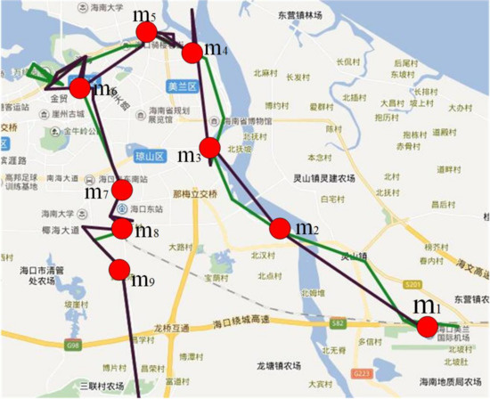
Figure 4.
Two trajectories moving together with different sampling rate.
| Algorithm 1: Trajectory Similarity |
| Input: Output: 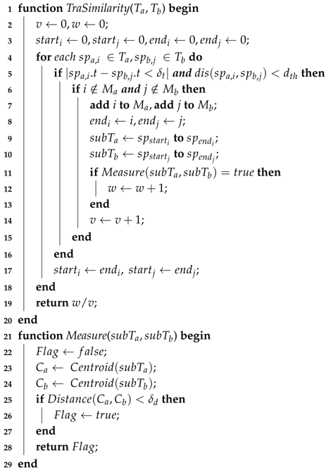 |
The core concept of the algorithm is to divide an entire trajectory into sub-trajectories by the matching points on two trajectories, then measure the similarity of two trajectories based on the distance between centroids of each pair of sub-trajectories. For the two trajectories in Figure 4, the trajectory similarity calculated by the proposed algorithm is 0.693, compared with 0.455 for LCSS, 0.102 for ED, 0.183 for normalized DTW. So those algorithms are obviously not suitable in this situation.
Definition 3.
(Matching Point): Given trajectory and , and are the stay points of and respectively. is a time threshold. and are called matching points if:
- (1)
- (2)
where is the distance of the two points.
The algorithm consists of two functions. The function TraSimilarity (Line 1–20) is to find the matching points and then divide trajectories into sub-trajectories by the matching points. and are the set of the matching points in and . The function Measure (Line 21–29) is to judge if the two sub-trajectories are similar by calculating the distance between two centroids of sub-trajectories. First, we try to find the matching points of the two trajectories (Line 5). To avoid the situation that one point can be matched with two different points in another trajectory, we choose the first matching point in another trajectory as the start of the sub-trajectory (Line 6–7). To measure similarity of sub-trajectories with different sampling rate, we merge stay points on the sub-trajectory into a centroid and then use the distance between the two centroids to estimate the similarity of sub-trajectories (Line 25–27). In this way, the issue caused by different sampling rate can be addressed somehow. When the distance between the centroids of sub-trajectories is within , the two tourists are considered as a traveling companion in the sub-trajectory. Finally, the trajectory similarity of tourist a and b is denoted as:
where v is the number of sub-trajectories in the entire trajectories and w is the number of sub-trajectories on which tourist a and b are considered to be a traveling companion.
3.4.2. Accommodation Similarity
In the process of measuring similarity of the tourists, we consider not only the trajectories of the tourists, but also the places they stayed at night. Group movement patterns for tourists have distinct characteristics compared with other kinds of group movement patterns. For example, in the peak season, thousands of tourists crowd to famous scenic areas in Hainan at the same period, which leads to overlapped trajectories of different tourist groups in the daytime. So it’s hard to distinguish different tourists groups only by trajectory data. We try to find places tourists stayed at night to measure their similarities in accommodations. Generally speaking, a group of tourists will stay in the same place (maybe a hotel or a residence) at night which can be an important feature to measure the similarity of the tourists in a group.
The first step is to identity lodgings tourists stayed at each night. We define 21:00 to 9:00 as . It is obvious that tourists will spend most time in lodgings at Hometime. In the algorithm, we try to find the stay points with the longest duration at Hometime, and identified them as tourists’ lodgings. Supposing the length of stay for tourist a and b in Hainan is z nights which is calculated based on the timestamp difference of the first and the last records of each tourist, his/her lodgings in Hainan are denoted as a sequence of lodgings with date attached, i.e. . So we define the accommodation similarity of tourist a and b as
where denotes the number of same lodgings during z nights. Since we can not identify which specific hotel the tourist stays in when there are multiple hotels in the coverage area of the same base station, accommodation similarity is just one part of the similarity measurement.
3.4.3. The Similarity of other Features
Besides similarity measurements mentioned above, there are also other features related to travel behaviors that can be used to measure similarity. In this part, we extract the other two features which can help us identify the relationship between tourists in the groups, then combine the two features.
The first feature is the mobile phones’ home locations of the tourists, which can help to discover groups from a certain province. In CDRs, each record has a field to indicate the mobile phones’ home locations, for example, “301” represents Guangdong Province, “302” represents Shandong Province and so on. Utilizing this field we can easily discover tourists from the same province. Two tourists traveling together within the same tourist group are more likely to be from the same province.
The second feature is the number of days the tourists spent in Hainan which is also an important feature to distinguish different tourist groups. Generally, the members’ arrival and departure time in a group is usually consistent and the days they spent in Hainan will also be the same. We use the timestamp difference of the first and the last records of each tourist to calculate the maximum continuous days in Hainan as his/her second feature.
For tourist a and b, when the feature of tourist a and b has the same value, this feature is considered to be matched. We measure the similarity of the two features of tourists a and b by this equation:
where is the total number of features. Here the value of is 2. The is the number of matches of a and b.
3.5. Identify Group Tourists
After obtaining the similarity of tourist a and b which is denoted as , we need to judge whether a and b are a pair of traveling companions or not by the similarity vector.
We use two different methods to determine which pairs of the tourists are the traveling companions. The first method is a threshold-based method which sets a threshold to filter out the tourists who have low similarity with others in the candidate groups. We define , where are the weights of three features. and . If , the two tourists are identified as a traveling companion, otherwise not. Because of the complexity of travel behaviors, it is not so easy to choose the proper value of . We set four sets of weights with different threshold in our work to analyze.
In the second method, we apply safe semi-supervised support vector machines(S4VMs), a semi-supervised learning algorithm proposed by [45], after labeling some pairs of tourists manually, to identify the traveling companions. The algorithm uses unlabeled data to improve the performance of classification results when labeled data are limited.
The traveling companions that are in the same candidate group are identified as a real group. For example, in a candidate group , we find two pairs of traveling companions, namely and , then we consider the real group as .
4. Experiment and Results
4.1. Data Set and Experiment
In this paper, we use anonymized Call Detail Records (CDRs) and location-based data provided by one of the largest telecom operators in China. The data set contains more than 10 million anonymized mobile phone records from nearly half a million users in Hainan province in December 2015. Moreover, we crawled 17758 point of interests (POIs) in Hainan Province by using Baidu Map API, which indicate the location and category of venues like hotels, shopping malls, or scenic spots. Combined with POI data, the stay points can be annotated with their semantic information. For CDR data, accurate activity identification is a non-trivial problem [46,47]. However, in this paper, only places where the tourists visit or stay at night need to be annotated for tourists identification and their accommodation similarity measures. So we simplified the activity annotation by using the POI category with the maximum number of POIs in the coverage area of the base station with which the user connected. After extracting the users coming from provinces other than Hainan, we further select the users whose stay points include at least one scenic spots and consider them as tourists. Its total number is 115,098. To deal with the large-scale data, we use Apache Spark, a cluster computing framework for big data processing.
In the data preprocessing, the time threshold and distance threshold for stay points identification is set to be 10 min and 200 m respectively, slightly smaller than the commonly used threshold [48,49] in order to keep more stay points for trajectory similarity measurement. In the process of frequent groups mining, the interval of snapshots is set to be 30 min, which is long enough to ensure that the trajectory points of the tourists in the same group can be included in the same snapshots. The minimum size of candidate group M is 2 and the minimum snapshots for occurrence K is 4 which can avoid many accidental meeting events in scenic spots. In the process of trajectory similarity measurement, the time threshold of matching points is set to be 5 min which ensures the matching points of two sub-trajectories to be close enough to each other. The distance threshold between centroids of sub-trajectories should be large enough for the situation when members in one group are serving by the adjacent base stations. So we set to be 1 km.
In the process of identifying group tourists, for the threshold-based method, we choose four sets of weights, , with four similarity threshold , to examine the effects of different features and thresholds when calculating the similarity of the tourist pairs and identifying traveling companions.
4.2. Tourists Group Identification Results and Validation
By performing frequent itemsets mining on the collections generated from CDRs, excluding those who do not have stay points being annotated as scenic spots, we got 50,471 frequent itemsets and 43,894 of them are closed itemsets, totally 19,120 unique users. We treat the users who are not in the frequent itemsets as individual tourists, and its total number is 95,978. For each candidate group, we calculate the similarity of each pair of the tourists in the group.
We use the threshold-based method and S4VMs algorithm to get the real groups from the candidate groups. For S4VMs, 200 pairs of tourists were sampled and labelled manually as traveling companions or not, by plotting the trajectories on the map. Half of them are extracted from the frequent closed itemsets and the other half are picked from the whole data sets randomly. The results of the identified groups for the threshold-based method and S4VMs method are shown in Table 3. We selected four sets of weights, i.e., {0.5, 0.25, 0.25}, {0.25, 0.5, 0.25}, {0.25, 0.25, 0.5}, {0.33, 0.33, 0.33}, and four similarity thresholds , i.e., 0.6, 0.55, 0.5 and 0.45 for the threshold-based method. It can be seen that the group size in the results is not large, ranging from 2 to 8. Considering that the CDR data set comes from one telecom operator which market share is less than 20%, the actual group size may vary from about 10 to 40. Since the market share of the operator in different provinces are different, the group size may be affected by which province the group members came from. Although it is not easy to determine the exact size of the group, what we concerned about is the group behaviors rather than the group size.
Table 3.
Percentage of group tourists.
In Table 3, the total number of groups is the sum of all groups with a group size from 2 to 8. It shows that S4VMs can identify more tourist groups than the threshold-based method. For each method and the associated parameters, we illustrate the percentage of group tourists which defined as the ratio between the number of group tourists for each group size to the total number of the group tourists. The similarity threshold has a great impact on the number of identified groups. Higher similarity threshold means higher confidence of the discovered groups but will lead to lower number of groups. The threshold based method with weight2 {0.25, 0.5, 0.25} gets the least number of groups. This may be explained by that the requirements for accommodation similarity are more stringent. While the method with weight3 {0.25, 0.25, 0.5} obtains the most group number for the reason that the requirements for the last two features in the similarity measurements are easier to satisfy. It can also be noted that, with the aims of getting better understanding of the group movement behaviors, the proposed group identification method is relatively tight. In addition, only when more than one member in a group whose phone number belongs to this telecom operator, a group can be identified. So the number of discovered groups are smaller than expected, especially for large group size.
Since it is difficult to obtain the ground truth of the identified groups, we validated the results of the proposed methods in an indirect way. We first picked out the groups which travelled from Haikou city to Sanya city from the identified groups, in case they have the stay points located in both Haikou City and Sanya City. Then we designed an algorithm to detect the transportation mode of each group member. If the members in the same group have the identical transportation modes during their journey from Haikou to Sanya, they are very likely to be a traveling companion.
There are four major transportation routes between the two cities, namely the eastern expressway, the middle expressway, the western expressway and the railway. Firstly, the similarity between the tourists’ trip routes and the four major transportation routes is calculated. Then the travel time, average speed of the entire trip and the maximum distance deviated from the railway were also extracted as features. Finally, K-Means clustering is used to obtain the transportation mode of each tourist.
In Table 4, the match ratio of the transportation mode is shown. For each group size, we defined the matching ratio as the ratio of the number of the groups in which members share the same transportation mode to the total number of groups. It can be seen that, for the group size larger than 2, the groups identified by S4VMs can achieve 100% matching ratio, which means all the group members have the same transportation mode. So to some extent, this indirectly validates that the proposed methods can detect the tourist groups. S4VMs outperforms the threshold-based methods except for the case with weight2 when the similarity threshold is set to . The threshold based method with weight2 gets the highest matching ratio compared with the other three weights as expected. Higher similarity threshold can get better matching ratio. In the following analysis of the group tourists behaviors, we use the groups identified by S4VMs because it can achieve the best performance.
Table 4.
Matching ratio of the transportation mode
4.3. Travel Behaviors Analysis
With the results of the tourist groups identified by S4VMs method, We got 3509 groups, totally 7722 group tourists. As we mentioned above, the total number of the individual tourists are 95,978. In this sub-section, we analyze the travel behaviors of group tourists and individual tourists, including travel routes, travel time and so on. It should be noted that we identified the group and individual tourists from only one telecom operator’s CDR data set. Strictly speaking, it can only show the travel behaviors of users of this operators. However, in one tourist group, there will be users of other operators usually. So it would be more confident to infer travel behaviors of the whole population for group tourists than for individual tourists in this case.
4.3.1. Time to Visit the Scenic Spot
The time that tourists arrived at scenic areas is shown in Figure 5. We record the time when the tourists arrived at each scenic spot, and calculate the average percentage of the tourists at each time interval. The differences between group tourists and individual tourists can be seen clearly. More group tourists visited scenic areas before 9 o’clock than individual tourists. And in the afternoon, more individual tourists visited scenic areas than group tourists. This is reasonable because travel agencies often start their tours in the early morning, but individual tourists have a more flexible schedule so they are more likely to visit scenic areas in the afternoon.
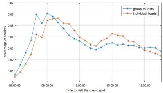
Figure 5.
Time to visit the scenic spot for group and individual tourists.
Figure 6 exhibits the average time spent in different scenic areas by group tourists and individual tourists. The scenic areas and the corresponding IDs are exhibited in Table 5. It can be seen that group tourists spend less time than individual tourists in most scenic areas, because the tourist groups often have a tight schedule so that they have much shorter visiting time at each location. But in Capital Outlets, a famous shopping mall, the average time spent by group tourists are longer than individual tourists.
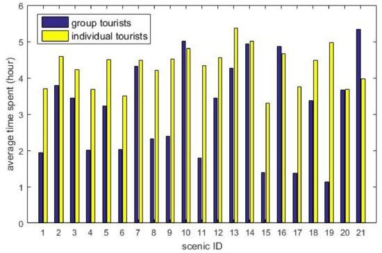
Figure 6.
Average time spent in different scenic areas.
Table 5.
Scenic area identifications and corresponding names.
4.3.2. Trip Distance
The trip distance is another important aspect of tourist behaviors. The trip distance of tourists is defined as the cumulative distance of their travel routes in Hainan province. We calculate trip distance of group and individual tourists from extracted trajectory data, and then count what is the percentage of the trips falling into each interval of trip distance. The results are shown in Figure 7. The group tourists represented in blue have a larger average trip distance than the individual tourists shown in red curve. This can be explained that the group tourists are likely to visit more places. The individual tourists prefer to stay at one area to relax.
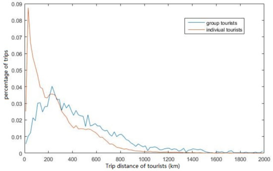
Figure 7.
Trip distance of tourists for group and individual tourists.
4.3.3. Origin and Destination
Besides the mobility of tourists, we are also interested in spatial distribution of tourists. We calculate the total number of tourist groups from different provinces and the result is shown in Figure 8. We found that Beijing, Sichuan and Heilongjiang are the top 3 provinces with the largest group of tourists.
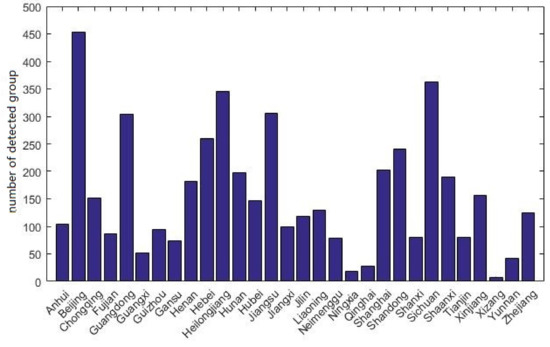
Figure 8.
Geographical distribution of group tourists, X-axis is provinces, Y-axis is the number of detected group from each province.
In addition to that, we are interested in the Origin-Destination matrix, which describes the tourists flow and the different distributions in each scenic areas. In Figure 9, the origin indicates the top 10 provinces which have the greatest number of tourist groups, and the destination is the scenic areas they visited. We can observe the top origins and destinations, as well as the trip distributions. Tourists from Sichuan and Beijing prefer to visit YaLong Bay and Dadonghai than other scenic areas. But few tourists visit Tropical Garden of Fauna and Dongshan Ridge.
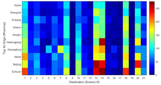
Figure 9.
OD matrix of group tourists. X-axis is the scenic ID of scenic areas and Y-axis is top 10 provinces with the most group tourists. (Top 1 is Sichuan, Top 10 is Hubei).
4.3.4. Popular Tourist Routes
To analyze the different travel preferences of group tourists and individual tourists, we try to mine the most popular scenic areas and popluar tourist routes in Sanya. In Figure 10, it can be seen that Dadonghai and YaLong Bay are the most popular scenic areas in Sanya.
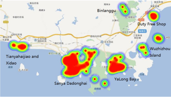
Figure 10.
Distribution of tourists in Sanya.
The popular route patterns of tourists are shown in Figure 11. The most popular route of group tourists is Yalong Bay⟶Dadonghai⟶Duty Free Shop. The top 2 route is Tianyahaijiao⟶Sanya Xidao⟶Dadonghai. The top 3 route is Tianyahaijiao⟶Sanya Xidao⟶Nanshan Cultural Zone. Different from group tourists, the most popular route of individual tourists is Tianyahaijiao⟶Sanya Xidao⟶Dadonghai. The top 2 route is Tianyehaijiao⟶Nanshan Cultural Zone⟶YaLong Bay. The results indicate that group tourists are more likely to go shopping than individual tourists. And individual tourists are likely to choose to visit natural scenic areas.
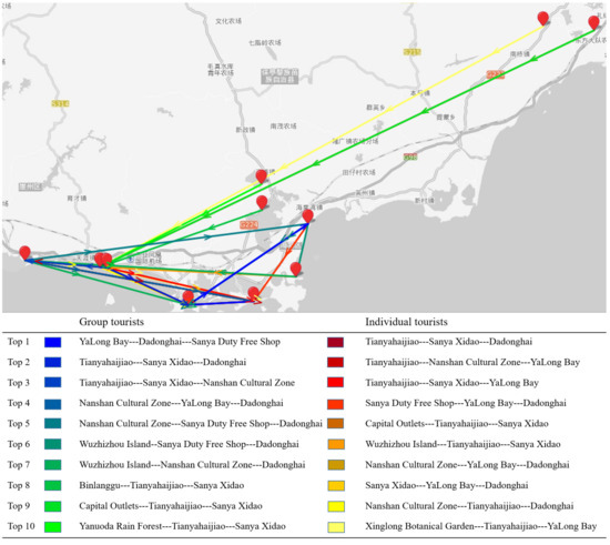
Figure 11.
Top 10 popular routes with three scenic areas.
5. Discussion
In this research, we proposed a threshold-based method and safe semi-supervised support vector machines (S4VMs) to find out group tourists after calculating the similarity vectors of tourists. Different weights and thresholds are applied in the threshold-based method to generate comparison results. The S4VMs method not only can discover more groups than the threshold-based methods, but also can get better performance when validating with transportation mode detection.
With the identified tourist groups, we presented the travel behavior patterns of group and individual tourists, including time to visit the scenic spot, trip distance, origin and destination matrix, and popular tourist routes. Group and individual tourists show relatively different travel behaviors. Compared to group tourists, more individuals prefer traveling in a more relaxed way, such as arriving at the scenic spots later, traveling less distance, etc.
Regarding to the travel behaviors, Phithakkitnukoon, S. et al. [36] also analyzed tourist behaviors in Japan, but they only take into account individual tourists and tourist flows at the aggregate level, not the real group. GMove in [14] presented a group-level mobility modeling using geo-tagged social media data. But it just groups the users that share the similar moving behaviors so as to discover a certain type of users, such as students or tourists. It is hard to differentiate the behavior of individual and group tourists.
6. Conclusions
In this work, we present a framework to identify tourist groups and analyze the travel behaviors of group and individual tourists by using call record details (CDRs) data. Compared to GPS data, CDR data is poor in spatial resolution with low sampling rate which makes it hard to obtain accurate trajectories of users. We propose a method called group movement pattern mining based on similarity (GMPMS) to identify tourist groups with sparse CDR data. A threshold-based method and a semi-supervised learning algorithm S4VMs are used to determine the traveling companions based on the similarity measurement. The proposed method is evaluated in the experiment by using CDR data set from Hainan province. We validate the identified groups in an indirect way by comparing the transportation modes of the group members.
The travel behaviors of group and individual tourists are analyzed based on the identified tourist groups. The empirical results derived from Hainan province indicate that these two kinds of tourists have different travel behaviors and preferences. Better understanding of tourist travel behaviors is importance for tourism planning and management. For example, as we discovered that group tourists spend far less time in some scenic spots than individual tourists, more activities suitable for group tourists can be designed by the scenic managers. Based on the proposed framework, POI or itinerary recommendation system for group and individual travel can be designed more specifically based on their different behavior profiles. For some security scenarios, discovery of traveling companions can be utilized to quickly find out a criminal suspect’s companion, which may also be helpful to public security system.
Author Contributions
X.Z., T.S. and H.Y. designed the framework and T.S. contributed to the group identification method. H.Y. and T.S. contributed to data processing. The group tourist exploration and the analysis of travel behaviors were conducted by H.Y. and T.S. The paper was reviewed by X.Z. Finally, the project administration and resources were provided by Z.H. and J.M.
Funding
This research received no external funding.
Acknowledgments
This work was supported by the Major Science and Technology Plan Project of Hainan Province, ZDKJ201808.
Conflicts of Interest
The authors declare no conflict of interest.
References
- Tsai, H.P.; Yang, D.N.; Chen, M.S. Mining group movement patterns for tracking moving objects efficiently. IEEE Trans. Knowl. Data Eng. 2011, 23, 266–281. [Google Scholar] [CrossRef]
- Zhou, Y.; Zhang, Y.; Ge, Y.; Xue, Z.; Fu, Y.; Guo, D.; Shao, J.; Zhu, T.; Wang, X.; Li, J. An efficient data processing framework for mining the massive trajectory of moving objects. Comput. Environ. Urban Syst. 2017, 61, 129–140. [Google Scholar] [CrossRef]
- Gudmundsson, J.; Van Kreveld, M. Computing longest duration flocks in trajectory data. In Proceedings of the 14th Annual ACM International Symposium on Advances in Geographic Information Systems, ACM-GIS’06, Arlington, VA, USA, 6–11 November 2006; Association for Computing Machinery: Arlington, VA, USA; pp. 35–42. [Google Scholar]
- Jeung, H.; Yiu, M.L.; Zhou, X.; Jensen, C.S.; Shen, H.T. Discovery of convoys in trajectory databases. Proc. VLDB Endow. 2008, 1, 1068–1080. [Google Scholar] [CrossRef]
- Li, Z.; Ding, B.; Han, J.; Kays, R. Swarm: Mining relaxed temporal moving object clusters. Proc. VLDB Endow. 2010, 3, 723–734. [Google Scholar] [CrossRef]
- Naserian, E.; Wang, X.; Xu, X.; Dong, Y. A framework of loose travelling companion discovery from human trajectories. IEEE Trans. Mobile Comput. 2018, 17, 2497–2511. [Google Scholar] [CrossRef]
- Liu, S.; Wang, S. Trajectory community discovery and recommendation by multi-source diffusion modeling. IEEE Trans. Knowl. Data Eng. 2017, 29, 898–911. [Google Scholar] [CrossRef]
- Tang, L.-A.; Zheng, Y.; Yuan, J.; Han, J.; Leung, A.; Hung, C.-C.; Peng, W.-C. On discovery of traveling companions from streaming trajectories. In Proceedings of the IEEE 28th International Conference on Data Engineering, ICDE 2012, Arlington, VA, USA, 1–5 April 2012; IEEE Computer Society: Arlington, VA, USA; pp. 186–197. [Google Scholar]
- Zheng, K.; Zheng, Y.; Yuan, N.J.; Shang, S.; Zhou, X. Online discovery of gathering patterns over trajectories. IEEE T. Knowl. Data Eng. 2014, 26, 1974–1988. [Google Scholar] [CrossRef]
- Zheng, Y. Trajectory data mining: An overview. ACM Trans Intell. Syst. Technol. 2015, 6, 29. [Google Scholar] [CrossRef]
- Sanches, D.E.; Alvares, L.O.; Bogorny, V.; Vieira, M.R.; Kaster, D.S. A top-down algorithm with free distance parameter for mining top-k flock patterns. In Proceedings of the Annual International Conference on Geographic Information Science, San Jose, CA, USA, 3–5 November 2018; pp. 233–249. [Google Scholar]
- Tang, L.-A.; Zheng, Y.; Yuan, J.; Han, J.; Leung, A.; Peng, W.-C.; Porta, T.L. A framework of traveling companion discovery on trajectory data streams. ACM Trans. Intell. Syst. Technol. 2013, 5, 3. [Google Scholar] [CrossRef]
- Wang, Y.; Luo, Z.; Xiong, Y.; Prosser, D.J.; Newman, S.H.; Takekawa, J.Y.; Yan, B. Discovering loose group movement patterns from animal trajectories. In Proceedings of the 11th IEEE International Conference on eScience, eScience 2015, Munich, Germany, 31 August–4 September 2015; Institute of Electrical and Electronics Engineers Inc.: Munich, Germany; pp. 196–206. [Google Scholar]
- Zhang, C.; Zhang, K.; Yuan, Q.; Zhang, L.; Hanratty, T.; Han, J. Gmove: Group-level mobility modeling using geo-tagged social media. In Proceedings of the Acm Sigkdd International Conference on Knowledge Discovery & Data Mining, San Francisco, CA, USA, 13–17 August 2016; pp. 1305–1314. [Google Scholar]
- Phan, N.; Poncelet, P.; Teisseire, M. All in one: Mining multiple movement patterns. Int. J. Inf. Techol. Decis. Mak. 2016, 15, 1115–1156. [Google Scholar] [CrossRef]
- Lee, J.-G.; Han, J.; Li, X. A unifying framework of mining trajectory patterns of various temporal tightness. IEEE Trans. Knowl. Data Eng. 2015, 27, 1478–1490. [Google Scholar] [CrossRef]
- Vlachos, M.; Hadjieleftheriou, M.; Gunopulos, D.; Keogh, E. Indexing multi-dimensional time-series with support for multiple distance measures. In Proceedings of the Acm Sigkdd International Conference on Knowledge Discovery & Data Mining, London, UK, 19–23 August 2003; pp. 216–225. [Google Scholar]
- Vlachos, M.; Gunopoulos, D.; Kollios, G. Discovering similar multidimensional trajectories. In Proceedings of the Proceedings of the 18th International Conference on Data Engineering (ICDE’02), San Jose, CA, USA, 26 February–1 March 2002; pp. 673–684. [Google Scholar]
- Keogh, E.; Ratanamahatana, C.A. Exact indexing of dynamic time warping. Know. Informat. Syst. 2005, 7, 358–386. [Google Scholar] [CrossRef]
- Lei, C.; Ng, R. On the marriage of lp-norms and edit distance. In Proceedings of the 30th International Conference on Very Large Data Bases, Toronto, ON, Canada, 31 August–3 September 2004; Volume 30, pp. 792–803. [Google Scholar]
- Lei, C.; Özsu, M.T.; Oria, V. Robust and fast similarity search for moving object trajectories. In Proceedings of the Acm Sigmod International Conference on Management of Data, Baltimore, MD, USA, 13–17 June 2005; pp. 491–502. [Google Scholar]
- Pierre-François, M. Time warp edit distance with stiffness adjustment for time series matching. IEEE Trans. Pattern Anal. Mach. Intell. 2008, 31, 306–318. [Google Scholar]
- Toohey, K.; Duckham, M. Trajectory similarity measures. Sigspatial Spec. 2015, 7, 43–50. [Google Scholar] [CrossRef]
- Magdy, N.; Sakr, M.A.; Mostafa, T.; El-Bahnasy, K. Review on trajectory similarity measures. In Proceedings of the 7th IEEE International Conference on Intelligent Computing and Information Systems, ICICIS 2015, Cairo, Egypt, 12–14 December 2015; Institute of Electrical and Electronics Engineers Inc.: Cairo, Egypt, 2015; pp. 613–619. [Google Scholar]
- Nakamura, T.; Taki, K.; Nomiya, H.; Seki, K.; Uehara, K. A shape-based similarity measure for time series data with ensemble learning. Pattern Ana. Appl. 2013, 16, 535–548. [Google Scholar] [CrossRef]
- Liu, H.; Schneider, M. Similarity measurement of moving object trajectories. In Proceedings of the 3rd ACM SIGSPATIAL International Workshop on GeoStreaming, IWGS 2012, Redondo Beach, CA, USA, 6 November 2012; Association for Computing Machinery: Redondo Beach, CA, USA, 2012; pp. 19–22. [Google Scholar]
- Wang, F.; Zhu, X.; Miao, J. Semantic trajectories-based social relationships discovery using wifi monitors. Pers. Ubiquitous Comput. 2017, 21, 85–96. [Google Scholar] [CrossRef]
- Ra, M.; Lim, C.; Yong, H.S.; Jung, J.; Kim, W.Y. Effective trajectory similarity measure for moving objects in real-world scene. In Information Science and Applications; Springer: Berlin/Heidelberg, Germany, 2015; pp. 641–648. [Google Scholar]
- Xue, M.; Wu, H.; Chen, W.; Ng, W.S.; Goh, G.H. Identifying tourists from public transport commuters. In Proceedings of the 20th ACM SIGKDD International Conference on Knowledge Discovery and Data Mining, KDD 2014, New York, NY, USA, 24–27 August 2014; Association for Computing Machinery: New York, NY, USA, 2014; pp. 1779–1788. [Google Scholar]
- Vu, H.Q.; Li, G.; Law, R.; Ye, B.H. Exploring the travel behaviors of inbound tourists to hong kong using geotagged photos. Tourism Manag. 2015, 46, 222–232. [Google Scholar] [CrossRef]
- Yang, L.; Wu, L.; Liu, Y.; Kang, C. Quantifying tourist behavior patterns by travel motifs and geo-tagged photos from flickr. Pervasive Mobile Comput. 2015, 18, 18–39. [Google Scholar] [CrossRef]
- Önder, I.; Koerbitz, W.; Hubmannhaidvogel, A. Tracing tourists by their digital footprints: The case of Austria. J. Travel Res. 2016, 55, 566–573. [Google Scholar] [CrossRef]
- Maeda, T.N.; Yoshida, M.; Toriumi, F.; Ohashi, H. Decision tree analysis of tourists’ preferences regarding tourist attractions using geotag data from social media. In Proceedings of the International Conference on IoT in Urban Space, Urb-IoT 2016, Tokyo, Japan, 24–25 May 2016; pp. 61–64. [Google Scholar]
- Maeda, T.N.; Yoshida, M.; Toriumi, F.; Ohashi, H. Extraction of tourist destinations and comparative analysis of preferences between foreign tourists and domestic tourists on the basis of geotagged social media data. ISPRS Int. J. Geo-Inf. 2018, 7, 99. [Google Scholar] [CrossRef]
- Sun, Y.; Li, M. Investigation of travel and activity patterns using location-based social network data: A case study of active mobile social media users. ISPRS Int. J. Geo-Inf. 2015, 4, 1512. [Google Scholar] [CrossRef]
- Phithakkitnukoon, S.; Horanont, T.; Witayangkurn, A.; Siri, R.; Sekimoto, Y.; Shibasaki, R. Understanding tourist behavior using large-scale mobile sensing approach: A case study of mobile phone users in Japan. Pervasive Mobile Comput. 2015, 18, 18–39. [Google Scholar] [CrossRef]
- Barkhordari, R.; Yusof, A.; Sohkim, G. Understanding tourists’ motives for visiting malaysia’s national park. J. Phys. Educ. Sport 2014, 14, 599. [Google Scholar]
- Caughey, D.; Warshaw, C. Dynamic estimation of latent opinion using a hierarchical group-level irt model. Political Anal. 2015, 23, 197–211. [Google Scholar] [CrossRef]
- Bos, E.H.; Wanders, R.B. Group-level symptom networks in depression. JAMA Psychiatr. 2016, 73, 411. [Google Scholar] [CrossRef] [PubMed]
- Nagin, D.S.; Odgers, C.L. Group-based trajectory modeling in clinical research. Annu. Rev. Clin. Psychol. 2010, 6, 109–138. [Google Scholar] [CrossRef] [PubMed]
- Man, A.; Davidyock, T.; Ferguson, L.T.; Ieong, M.; Zhang, Y.; Simms, R.W. Changes in forced vital capacity over time in systemic sclerosis: Application of group-based trajectory modelling. Rheumatology 2015, 54, 1464. [Google Scholar] [CrossRef] [PubMed]
- Moore-Russo, D.; Radosta, M.; Martin, K.; Hamilton, S. Content in context: Analyzing interactions in a graduate-level academic facebook group. Int. J. Educ. Tech. Higher Educ. 2017, 14, 19. [Google Scholar] [CrossRef]
- Wu, W.; Wang, Y.; Gomes, J.B.; Anh, D.T.; Antonatos, S.; Xue, M.; Yang, P.; Yap, G.E.; Li, X.; Krishnaswamy, S.; et al. Oscillation resolution for mobile phone cellular tower data to enable mobility modelling. In Proceedings of the 15th IEEE International Conference on Mobile Data Management, IEEE MDM 2014, Brisbane, QLD, Australia, 15–18 July 2014; Institute of Electrical and Electronics Engineers Inc.: Brisbane, QLD, Australia; pp. 317–324. [Google Scholar]
- Han, J.; Pei, J.; Yin, Y. Mining frequent patterns without candidate generation. In Proceedings of the 2000 ACM SIGMOD—International Conference on Management of Data, Dallas, TX, USA, 16–18 May 2000; pp. 1–12. [Google Scholar]
- Li, Y.-F.; Zhou, Z.-H. Towards making unlabeled data never hurt. IEEE Trans. Pattern Anal. Mach. Intell. 2015, 37, 175–188. [Google Scholar]
- Yin, M.; Sheehan, M.; Feygin, S.; Paiement, J.F.; Pozdnoukhov, A. A generative model of urban activities from cellular data. IEEE Trans. Intell. Transport. Syst. 2018, 19, 1–15. [Google Scholar] [CrossRef]
- Tu, W.; Cao, J.; Yue, Y.; Shaw, S.-L.; Zhou, M.; Wang, Z.; Chang, X.; Xu, Y.; Li, Q. Coupling mobile phone and social media data: A new approach to understanding urban functions and diurnal patterns. Int. J. Geogr. Inf. Sci. 2017, 31, 2331–2358. [Google Scholar] [CrossRef]
- Widhalm, P.; Yang, Y.; Ulm, M.; Athavale, S.; González, M.C. Discovering urban activity patterns in cell phone data. Transportation 2015, 42, 597–623. [Google Scholar] [CrossRef]
- Jiang, S.; Fiore, G.A.; Yang, Y.; Ferreira, J., Jr.; Frazzoli, E.; Gonzalez, M.C. A review of urban computing for mobile phone traces. In Proceedings of the Acm Sigkdd International Workshop on Urban Computing, Chicago, IL, USA, 11–14 August 2013; p. 2. [Google Scholar]
© 2019 by the authors. Licensee MDPI, Basel, Switzerland. This article is an open access article distributed under the terms and conditions of the Creative Commons Attribution (CC BY) license (http://creativecommons.org/licenses/by/4.0/).