Article

Impact of the Scale on Several Metrics Used in Geographical Object-Based Image Analysis: Does GEOBIA Mitigate the Modifiable Areal Unit Problem (MAUP)?

UMR ESPACE 7300, CNRS, Department of Geography, 74 rue Louis Pasteur, 84029 Avignon CEDEX, France
*
Author to whom correspondence should be addressed.
ISPRS Int. J. Geo-Inf. 2019, 8(3), 156; https://doi.org/10.3390/ijgi8030156
Submission received: 30 September 2018 / Revised: 1 January 2019 / Accepted: 24 February 2019 / Published: 22 March 2019
(This article belongs to the Special Issue GEOBIA in a Changing World)

Abstract

:
Using two GEOBIA (Geographical Object Based Image Analysis) algorithms on a set of segmented images compared to grid partitioning at different scales, we show that statistical metrics related to both objects and sets of pixels are (more or less) subject to the Modifiable Areal Unit Problem. Subsequently, even in a same spatial partition, there may be a bias in statistics describing the objects due to some size effect of the pixel samples. For instance, pixels homogeneity based on Grey Level Cooccurrence Matrices (GLCM), Landscape Shape Index, entropy, object compacity, perimeter/area ratio are studied according to scale. The approach consists in studying the behavior of a given statistical metrics through scales and to compare the results on several image segmentations, according to different partitioning processes, from GEOBIA (Baatz & Schäpe algorithm and Self Organizing Maps) or using reference grids. We finally discuss about the relationship between GEOBIA metrics and scale. By analysing object shape and pixels composition from different metrics points of views, we show that GEOBIA does not always mitigate the Modifiable Areal Unit Problem.

1. Introduction

1.1. The Modifiable Areal Unit Problem

The Modifiable Areal Unit (MAUP) has two related aspects depending on the way we consider surface units [1]: scale or spatial partitioning, which are tightly related to multilevel modeling [2,3,4]. The first aspect is in a vertical dimension (scaling), while the second one is in a horizontal dimension (zoning). Both lead to the same problem: the way spatial entities are aggregated or delineated [5] provides a spatial partition whose polygons organization and shapes have a non negligible impact on any (geo)statistics measuring the parts and the whole, according to different boundary definitions (cf. [6]). This issue is shared by many disciplines and domains (see Figure 1) with different highlights, although it mainly results in a statistical bias. It is intimately related to the ecological inference problem or fallacy formulated by Robinson in 1950 [7] to denounce the use of aggregated statistics to infer knowledge on individual behavior [8].
In economy and medicine, a close problem was identified in 1951 as the Simpson’s paradox [9] using contingency tables. It shows that the way we (re)sample the data can lead to opposite conclusions. The issue becomes spatial once we deal with located data. We then focus on geographical partitioning and face to the Change Of Support Problem (COSP) [10,11]. It draws a set of problems related to the change of support of the data (for instance, points to polygons, polygons two points). Beside a reference partition with a certain scale and accuracy, it is possible to infer new partitions, by upscaling (spatial data aggregation) or downscaling (generally under strong assumptions of disaggregation) [12]. Since this problem was discovered by Gehlke and Biehl in 1934 [13] and inspired from the primal work of Yule [14], several works attempted to tackle it and proposed solutions, but none of them are consensual [15,16].
Openshaw recommended different ways to deal with the MAUP: ignoring the problem due to its insolubility, assuming it or even using it as a powerful analytical device to enrich geographical knowledge, by considering many scales and developing strategies of data (dis)aggregation. A solution would be to consider only the finest partition at the individual granularity. Unfortunately, the appropriate data are not often available. Another approach consists in adapting the metrics, for instance by weighting the correlation by the spatial units size [17] or any information related to variance or spatial auto-correlation [18]. Given a certain objective related to variance, it is also possible to build the best fitted partition at an individual level [19,20,21]. Complementary approaches were developed to get the optimal scale or spatial resolution [11,22,23,24,25]. This point out the strong relation that exists between scale, spatial partitioning and map generation. Sensitivity analysis of the spatial statistics depending on the MAUP can also be processed using random (re)sampling [11,24,26] or Bayesian statistics [27].
In conclusion, MAUP sounds as a difficult (geo)statistical problem, especially in spatial analysis where its effect is, on the one hand, visible and quite easy to detect, but on the other hand, impossible to definitely solve and therefore very frustrating for spatial analysts. That is why reducing the MAUP effects states as an essential stake and often becomes an argument to defend or justify the use of a particular partitioning or segmentation method, for instance in image analysis.

1.2. Relation between Modifiable Areal Unit Problem and Geographic Object Based Image Analysis

Geographic Object Based Image Analysis (GEOBIA) has to deal with several issues which can be considered as “burning research questions, research need and outlook” as expressed in the book edited by T. Blaschke, S. Lang and G. J. Hay in 2008 [29]. Related to quality in a general meaning, one of these issues is the reliability and the relevance of the statistics used to draw the correct objects boundaries. Indeed, since the number of pixels can strongly change at a given scale, and due to the major advantage of GEOBIA to find objects with different size and shape, any statistical metrics describing those objects must be handled and interpreted with a particular caution regarding scale.
In several reference articles [30,31,32], GEOBIA is enhanced as a good alternative to pixel oriented image analysis. Delineation, classification, segmentation, object identification, partitioning or scale management are some of the capabilities of GEOBIA to “derive meaningful objects”. But what is a meaningful spatial object? On a semantic point of view, it is something that refers to symbolic representation and language, something anchored, apprehensive ans shared by people (e.g., a forest or a house on an image or on a map). On a more technical point of view in the field of image analysis, it is a composition, a texture and an organization of pixels with different radiometric signatures, that draws a contour (the object boundary) and a polygon over which the texture shows significant differences, this discontinuity enabling to pass to another object. To provide a meaningful spatial partitioning, the resulting object shape and composition should be identical or at least quite similar in a given class of objects and at a given scale. Although the role of human perception and interpretation remains crucial to fix the final segmentation, spatial analysts have to base their decision on their knowledge and also on objective metrics [33], especially if one wants to automatize mapping. So, notably in GEOBIA, (good) map generation is tightly linked to (good) object identification.
Since an object from a segmentation process is mainly made of two complementary features—itself and the set of pixels it comprises—and regardless of scale issues and object semantic uncertainty, this leads to deal with two types of metrics, whether we consider the object or its pixels. Those metrics are well-known and available in different software of GEOBIA (e-Cognition, GEODMA, etc.). A first set of metrics describes the objects geometry in the spatial partition: size, shape, orientation, compacity, etc. A second set of metrics provides information about the internal texture and composition of the object: pixels values (in different colors) average, homogeneity, amplitude, etc. Those two complementary dimensions are very fruitful for the spatial analyst to polish up his/her classification. For instance, it becomes quite easy to extract all the swimming-pools from a image: the pixel color is most of the time blue and the object shape is regular (in a quite narrow range of a rectangle surface) with a high value of compacity. However, many of the observed spatial objects are not so simple and accurate [33]. They mix together, especially if we look at them at different scales: a tree belongs to a cops, that belongs to a moor, that belongs to a larger natural or agricultural space. So should we study how meaningful can be objects through scales, using those different types of metrics we previously mentioned.

1.3. Objectives

In the chapter 1.4 of the previously cited book [29], page 81, it is written that “object-based approaches represent viable solutions to mitigate the Modifiable Areal Unit Problem, since they focus the analysis on meaningful geographical objects rather than arbitrary defined spatial units i.e., individual pixels”. On the page 83, we can read: “image-objects are less sensitive to MAUP than units that do not keep a correspondence with the structure of the phenomenon under study” [34]. This statement leads us to question about the real capacity of GEOBIA to deal with the MAUP. Beyond, it is of great interest to study in details the relationship between GEOBIA metrics and scale.
At a first glance, GEOBIA seems indeed to be a promising way to manage, even reduce, the MAUP, because it allows to homogenize the pixel values in the polygons and subsequently to reduce the pixel values variance within objects, while increasing the variance between the objects of a spatial partition. Our assumption, which we think it may be shared by many image and spatial analysts, is that using GEOBIA, we expect to design more accurate maps, that better identify objects and thus spatial discontinuities between them. Implicitly, in image analysis, this means that an object is something quite homogeneous in its signature and different from other objects in the neighbor (it is a question of variance). Playing with scale allows to provide rather various aspects of what is “homogeneity”. Homogeneity can be (on an extreme point of view) an equality of pixel values in an object, but also a regularity in the pixel value distribution (similar objects share the distribution). In our case, we propose to focus on the first approach using a series of metrics that objectively describe the objects through scales, especially their homogeneity. In addition, we propose to study the objects shape. This provides a set of two different metrics which describe:
  • the texture of the objects according to their pixels composition, that deals with homogeneity purpose;
  • the shape of objects, that has no concern with homogeneity, but that may help in the readability of the map with non-coarse and compact objects).
This article finally tackles two questions:
  • What is the relationship between some of the GEOBIA metrics and scale?
  • Is it true that GEOBIA mitigates the MAUP, and, if so, in what way and what extent?
Using a series of experiments with several metrics, partitions and scales, we discuss these issues in this article.

2. Methodology

We study different partitioning processes in a well-known mountainous area (Mont Ventoux, France) using a single simple aerial photography and several metrics. As mentioned in the introduction, these metrics characterize objects themselves or pixels included in those. Our purpose is not to analyze all the possible spatial partitions. It is rather to study the behavior of a given statistical metrics following regular scaling ranks and to compare the results on several image segmentations, according to very different partitioning processes, i.e., a grid and partitions generated by several algorithms used in GEOBIA.

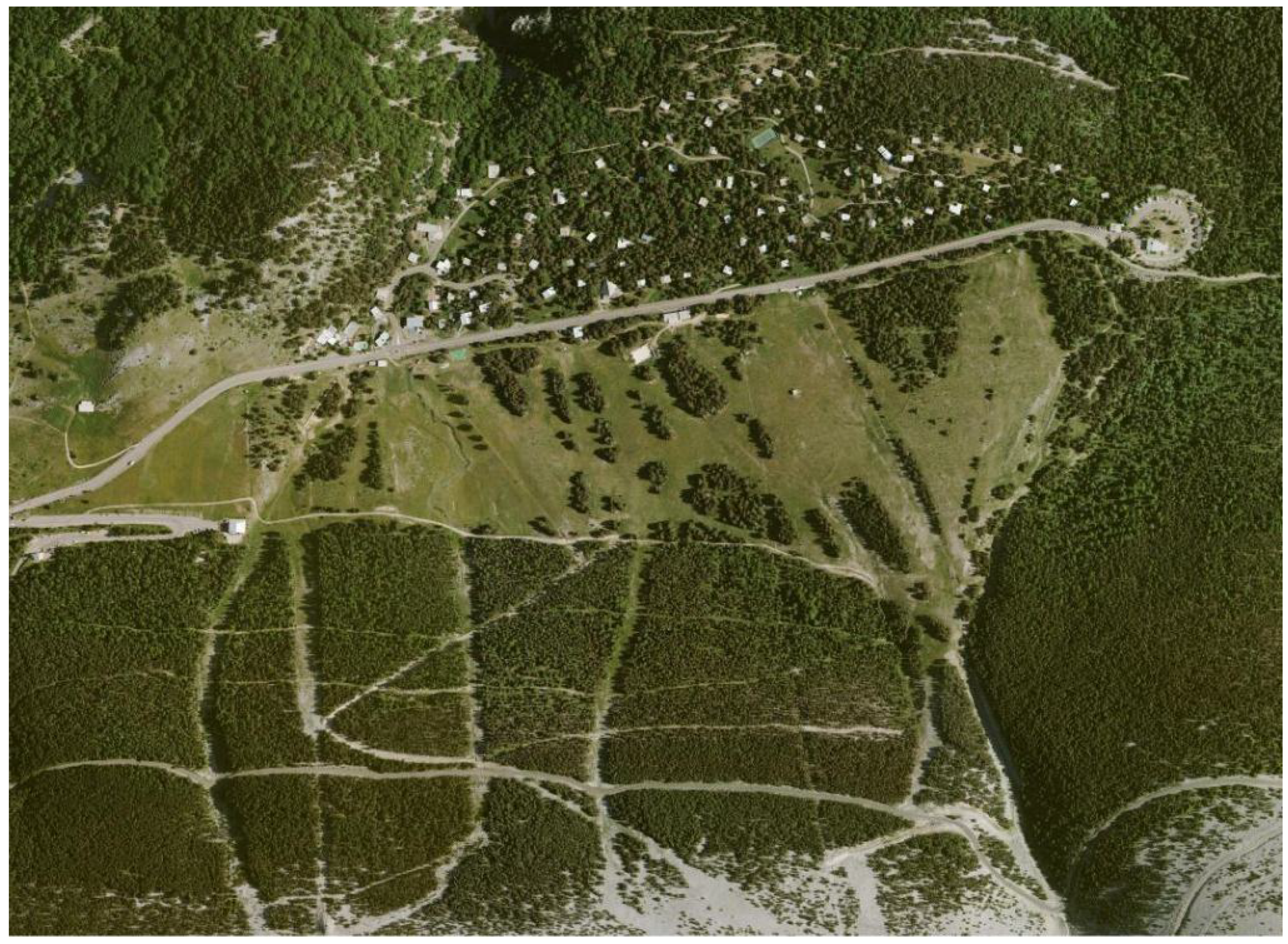
2.1. Material and Data

The reference is a 960 × 700 pixels aerial image (cf. Figure 2) with a pixel resolution of 2 m from the Institut Géographique National (IGN, French mapping and survey agency) web portal. It is an interesting location, because there are distinct land uses: forest, meadows, copses, alpine ski runs, pathways, road, fallen rocks and chalets [35]. Also, there are little vs large, long linear vs more compact objects. Both pixel values and object characteristics can be studied.
We used the free-ware GEODMA [36]. This software is useful for little images processing and sufficient for our methodological survey. It provides interesting metrics according to several algorithms. We focus on two distinct and complementary approaches:
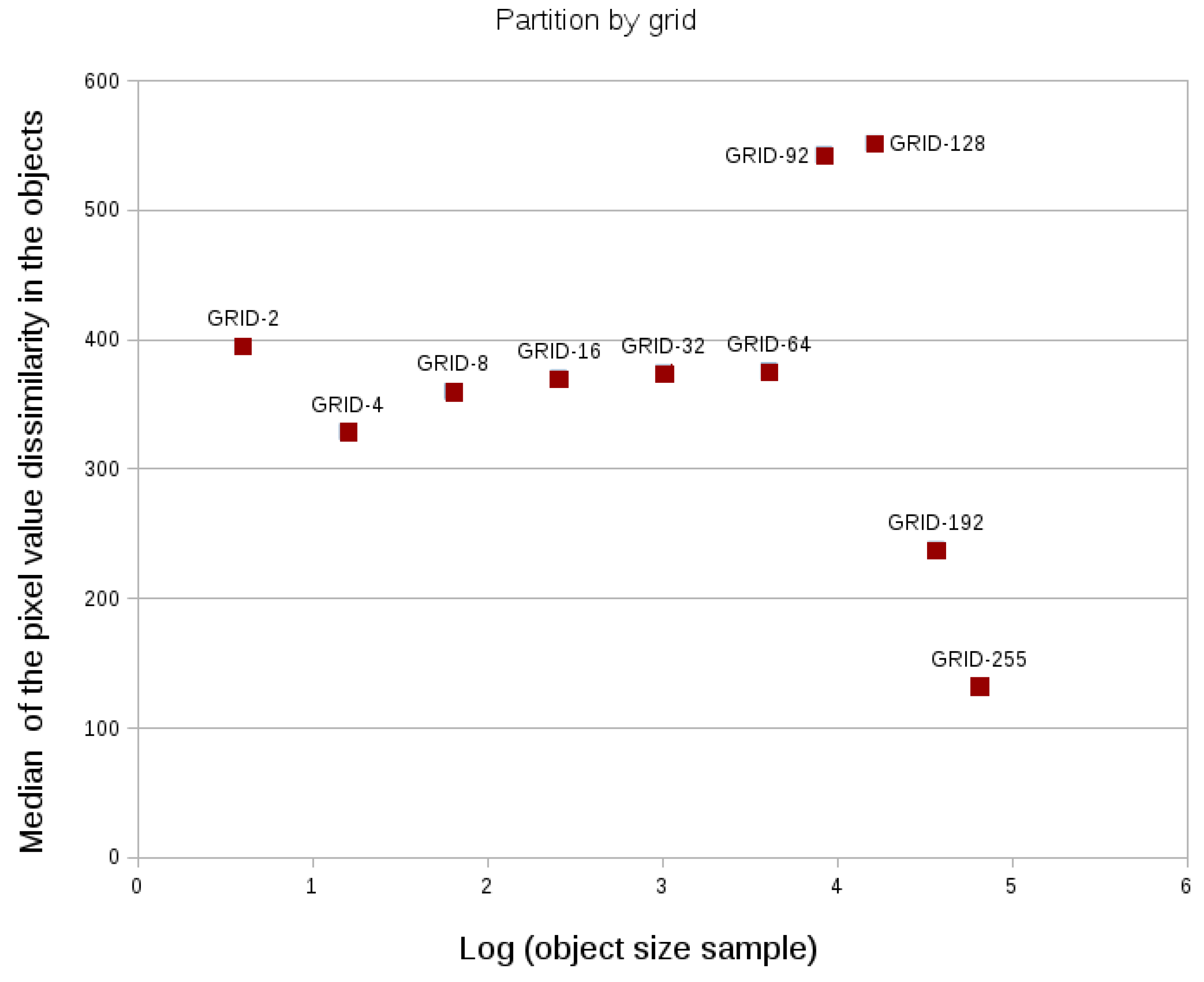
  • A series of reference non optimized partitions in grids: GRID-N, where N is the number of columns or rows of the grid, with a various quantity of polygon rectangles (2 × 2, 4 × 4, 8 × 8, 16 × 16, 32 × 32, 48 × 48, 64 × 64, 92 × 92, 128 × 128, 192 × 192 and 255 × 255) exemplified by the Figure 3 (GRID-16 with 16 × 16 cells);
  • A series of segmentations generated by two GEOBIA algorithms:
    -
    the Baatz and Schape algorithm [37]: BS-S, where S is the varying scale parameter in GEODMA, see Figure 4 and Figure 5; for most of the BS-S partitions, the color and the shape parameters are fixed;
    -
    Self Organizing Maps adapted to GEOBIA [38,39]: SOM-R-A-K, where R is the radius of the neighborhood Gaussian function of the neuron, A is alpha, the learning rate used to update the neural network and K is the radius of the geographical best matching unit to be searched (Figure 6).
Concerning the Baatz and Schäpe algorithm and for the resulting segmentations to be comparable, for most of the partitions, the color parameter is fixed to 40 and the shape parameter to 30, while the scale parameter S can change over a large range: 5, 6, 7, 10, 15, 20, 40, 50, 70, 100, 150, 200, 250. This means that the impact of the color and the shape input parameters is somehow equivalent, while the effect of scale is emphasized due to a very large range (from 5 to 250). There are however three particular cases, labelled BS-50-1, BS-50-3 and BS-50-3 where the scale is fixed to 50 (a “middle” scale) and the [color & shape] parameters are respectively set to [40 & 100] (predominance of the shape in delineating), [100 & 100] (predominance of the color) and [100 & 30] (joint importance of color and shape compared to scale). These three specific cases introduce an important change in color or shape that may have an influence on the resulting metrics values. The Baatz and Schäpe algorithm is based on a region growing and on a multi-resolution procedure. According to the region growing part, the scale value should more or less correspond to the half of the maximum width of the objects in pixels. What is important to keep in mind is that larger the scale, bigger the objects (it is not a cartographic scale). In GEOBIA practice, the scale and also color and shape parameters must be tuned in such a way they provide the “best” partition in the eyes of the spatial analyst. On the contrary, our approach is rather automatic and systematic: we shall interpret the metrics values behavior through scales. Moreover, we added 3 segmented images at scale 50 with varying color and shape weights to check how strong may be the color or shape parameters effect in the compared results.
We will not provide much more information about the Baatz and Schäpe algorithm or the Self Organizing Map parameters. Many other algorithms with parameter variations could have been used and compared, but it is not the purpose of this article. As we shall see, what is of interest here is mainly the measurement differences between partitioning based on grid versus GEOBIA.
The Figure 3 depicts the way the image is partitioned using a grid. All the pixels inside a grid cell will be considered for computation. The partitioning is completely arbitrary, although it is topological (regular rectilinear delineation). A grid of law spatial resolution will provide a larger set of grid cells and in parallel a lower number of pixels in each. In this particular case, the number of pixels is the same in all the grid cell.
Figure 4 and Figure 5 show very different spatial partitions. When scale decreases (from 70 to 20), the number of objects increases and subsequently, the averaged number of pixels in those objects is lower. These segmentation processes provide different distributions of homogeneous objects.

2.2. Metrics through Scales

In our study, we consider statistics about objects composing the image and about pixels included in those objects, given a certain spatial partition.

2.2.1. Metrics

Among many statistical metrics calculated using GEODMA (see [36] for details about these metrics), we selected a few of them, whether they concern the pixels composition in the objects or the objects themselves (cf Table 1):
  • For the pixel statistics on spectral values in the objects:
    -
    Homogeneity of the pixel values in objects (pixel homogeneity in the Grey Level Co-occurrence Matrix, GLCM, [40])
    -
    Dissimilarity of the pixel values in objects (contrast in the GLCM)
    -
    Entropy of the pixel values in objects (Shannon entropy)
    -
    Amplitude, i.e., difference between the lowest and the highest values of the pixels in objects
  • For the object shape description:
    -
    Compacity of the polygon, ratio of the area of the shape to the area of a circle (the most compact shape) having the same perimeter
    -
    Ratio perimeter/area of the polygon
    -
    Landscape Shape Index of the object, measure of the normalized patch geometric complexity by a normalized ratio of patch perimeter to area in which the complexity of patch shape is compared to a standard shape (square) of the same size [41]

2.2.2. Image Processing

For all the metrics and given a partition from a grid or from a GEOBIA algorithm, we proceed the same way in a first stage:
  • Generate a partition with a given method (GRID or GEOBIA algorithm);
  • Process the chosen metrics per object (compacity, ratio perimeter/area and shape index) and according to pixels distribution in each object (homogeneity, dissimilarity, entropy and amplitude);
  • Get a table with all the statistics of the objects in the partition;
  • Map the results in a Geographical Information System (QGIS).

2.2.3. Statistical Analysis

Then, in a second stage, we compare the statistical results for all the partitions by plotting:
  • the median of the object metrics (which summarizes the value of the given metrics in a given scale with a given segmentation method);
  • the object sample size according to the series of scales: the sample size increases when the number of the counted objects decreases.

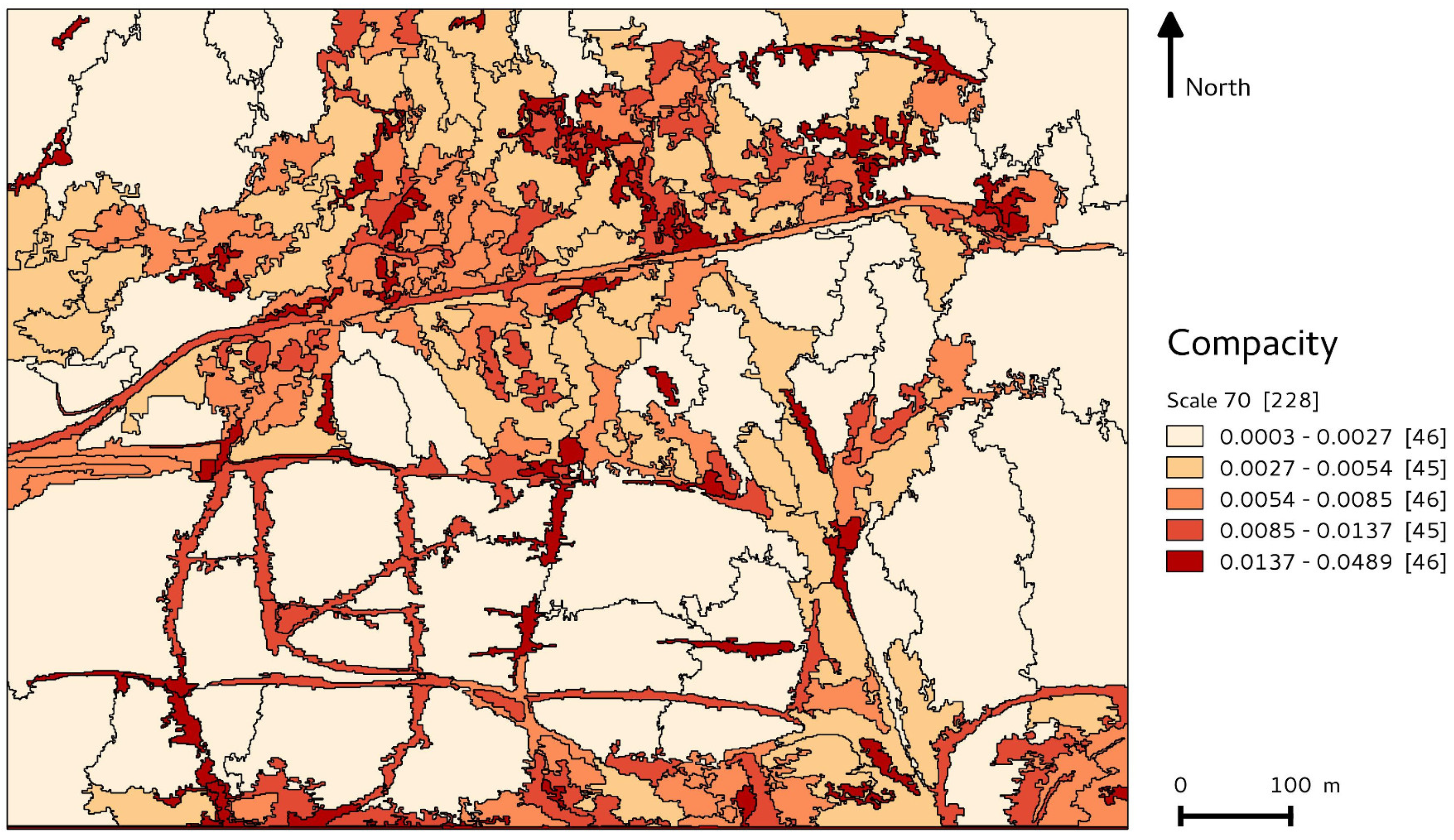
3. Illustration by Maps

In this section, we provide several maps from the numerous partitions we obtained, to illustrate how some object metrics look like on maps. You will notice that the object shape and size and the metrics classified values are very different according to the scale, to the algorithm used and the metrics itself, from an imposed grid to a partition obtained using GEOBIA.
The first map in Figure 7 depicts the median amplitude of the pixel values in each rectangle of the grid 16 × 16, discretized in quantiles. We can find out the structure with its global variance: along the road and in the rocky areas, the amplitude is high at this scale. Indeed, the pixel values are very different in the corresponding grid cells. At the opposite, the pixel value amplitude is low when considering the large forest and pasture areas.
The three following maps show respectively the median of:
  • the object compacity on a segmentation using Baatz and Schape algorithm, at scale 70 (Figure 8), with a quantile discretization of the resulting classes,
  • the object shape index on a segmentation using Baatz and Schape algorithm, at scale 20 (Figure 9), with a discretization of the resulting classes using equal ranges,
  • the pixel value homogeneity on a segmentation generated by a Self Organizing Map (Figure 10), with a quantile discretization of the resulting classes.
The Figure 8 illustrates the object compacity, which is low for large forest and pasture areas and high for more narrow roads, copses and edges.
As we noticed, it is not obvious to observe a clear and general relation between the area or the shape of the objects and the color of the class (values of the metrics for the objects on the map), whatever the scale, the metrics and the partitioning method. Since the number of pixels accounted in the object is directly depending on the size of the object and also on the number of objects in the segmented map, we propose to plot the different metrics statistics according to the number of objects delineated. By this way, we can study the relationship between the metrics value and the scale.

4. Statistical Results and Discussion

We need a global statistical overview to answer to the question: is there a relation between scale and metrics statistics?

4.1. Statistical Calculation

To do so, and once all the metrics are computed, we apply the following process, repeated for all the partitions or segmentations:
  • From the statistical table and for all the objects, calculate the global metrics statistics of the objects in the partition; for a given scale and a given partition, the median of each metrics is provided;
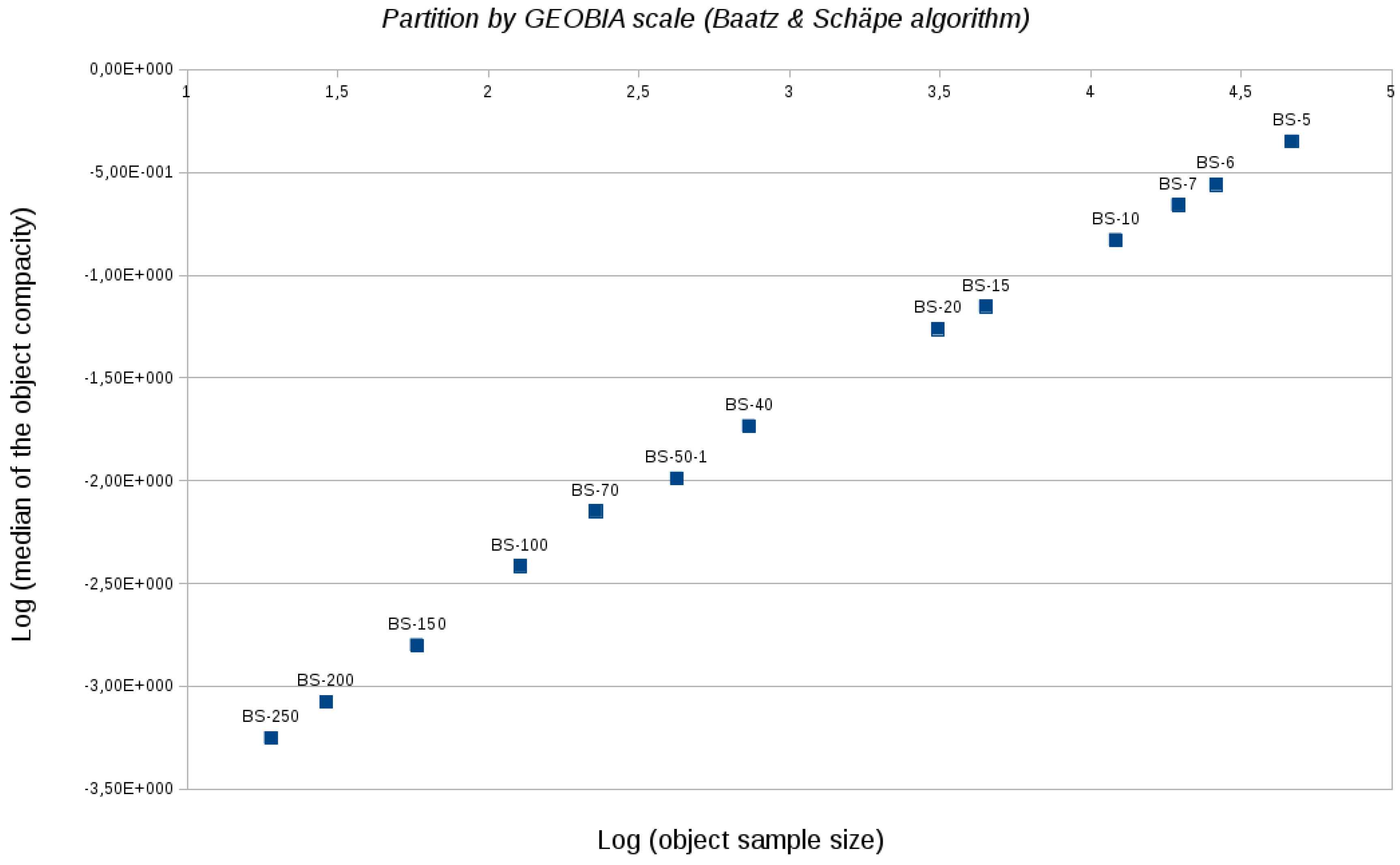
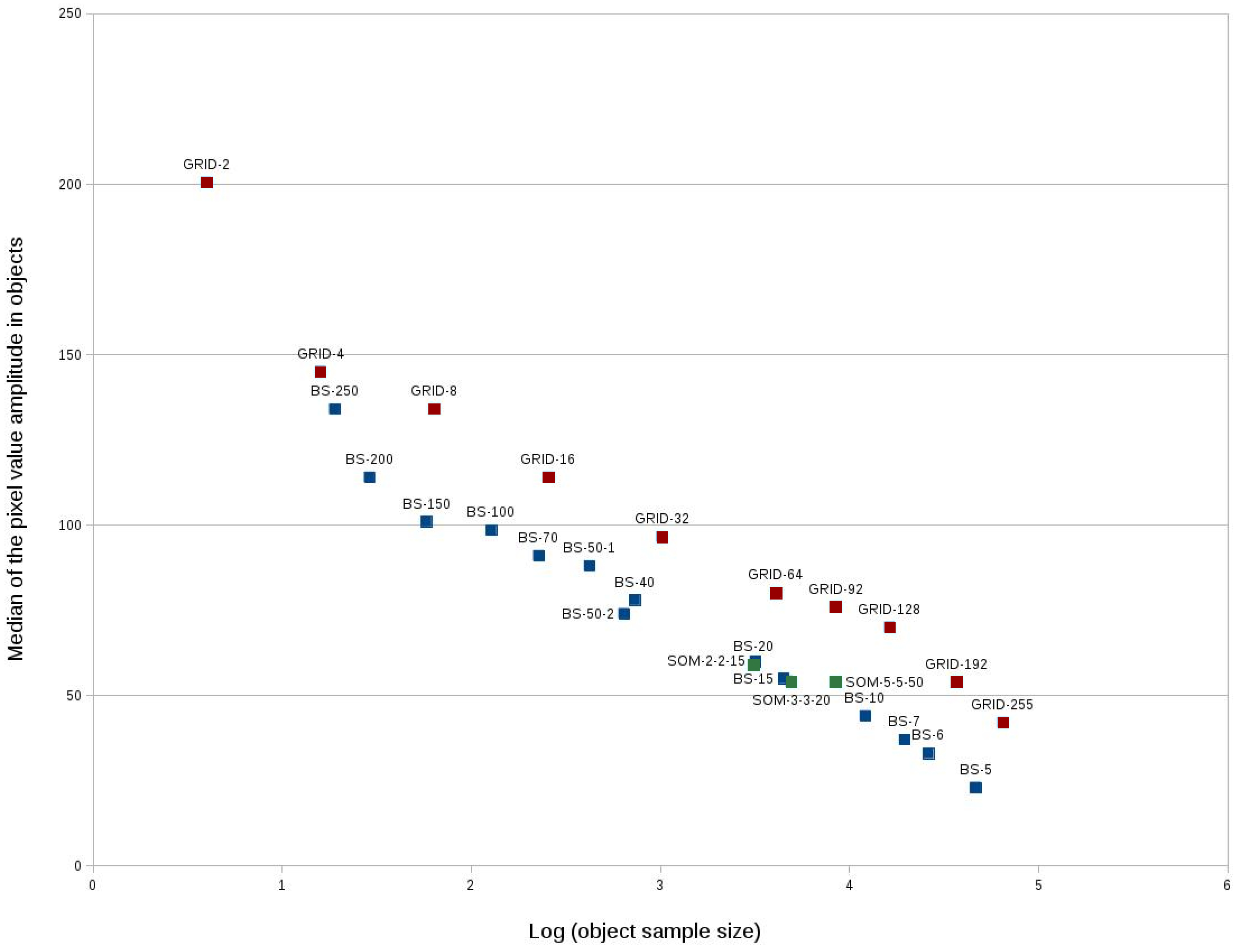
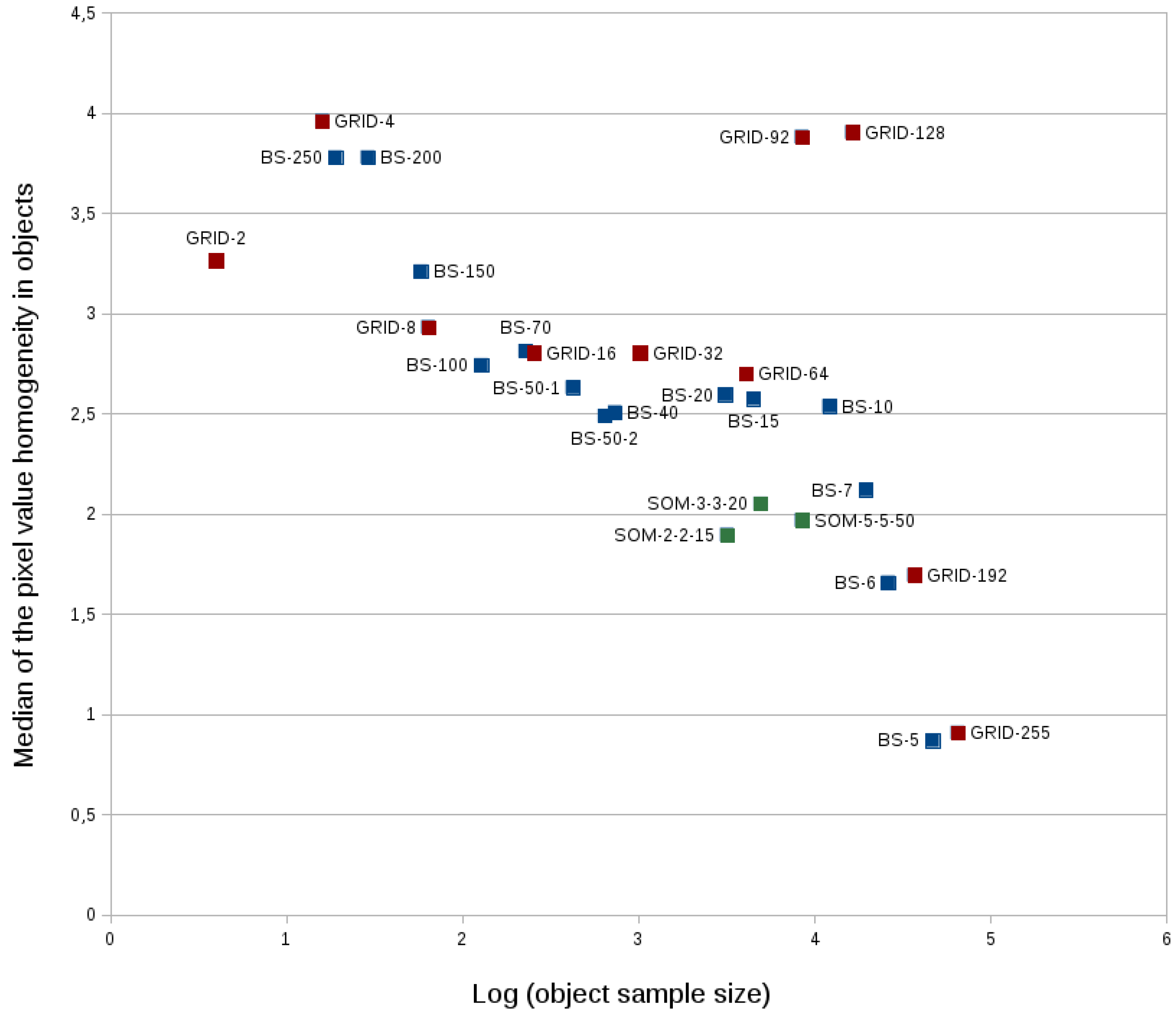
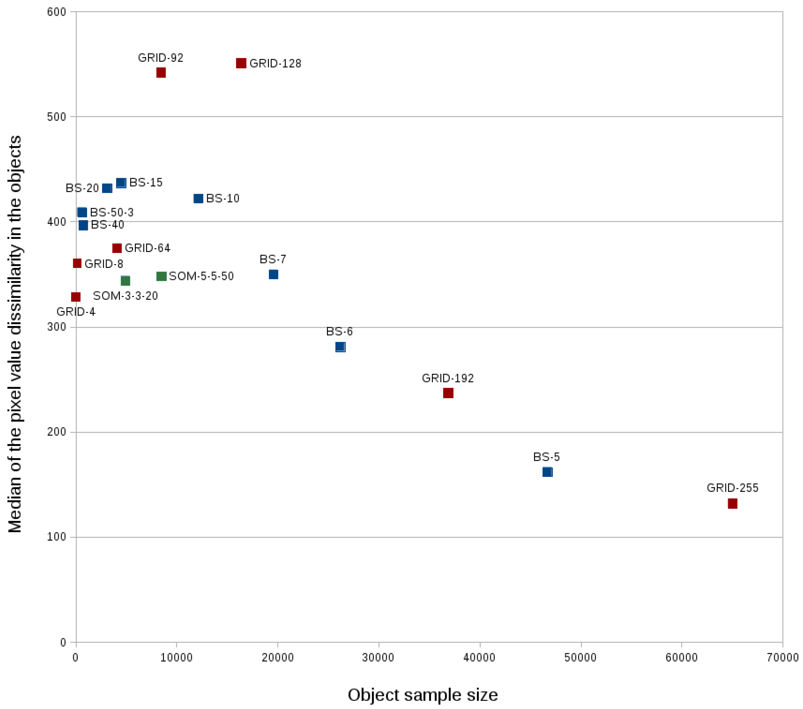
  • Plot systematically the metrics statistics on the Y axis and the object sample size on the X axis, i.e., the number of polygons in the partition, to emphasize the relationship;
  • If it is difficult to graphically separate the different cases from each other, transform the data using a log, that keeps the data sequence monotony and clarifies the points cloud;
  • By interpretation, check if there is a gain using GEOBIA and a scale effect or not, by comparing geometrical partitions (grids) to optimized segmentations (GEOBIA).
Let us analyze step-by-step the results we obtained with the different configurations of partitioning. We assigned three different colors to represent the metrics values provided by the different partitioning processes on the plots:
  • blue for BS algorithm results,
  • green for the SOM results,
  • red for the grid results.

4.2. Global Relationship between Metrics Values and Object Sample Size: Most of the Metrics Are Subject to the MAUP

Not surprisingly, we observe for most of the studied metrics and partitions that there is a strong relationship between the metrics value and the scale (object sample size). This is notably visible in the plots of the Figure 11, Figure 12, Figure 13, Figure 14, Figure 15 and Figure 16 with ratio perimeter/area, object compacity, pixel value amplitude, homogeneity or dissimilarity. It is due to the well-know ecological effect noticed in the literature and introduced in the first section. When the number of objects decreases, the averaged number of pixels in the objects increases and the variance of their metrics values decreases. This illustrates the mechanical impact of upscaling on spatial statistics, and in particular for GEOBIA measures, including object shape and pixels texture.

4.3. Segmentation Improvement by GEOBIA for Some Metrics

With a first glance at the Figure 11 and Figure 12, we can see that GEOBIA improves the value of several metrics, using BS or SOM algorithms. As a matter of fact, all the median values of object compacity or perimeter/area ratio are better than the ones calculated within the grids, especially for the segmentations generated with the SOMs, which provide metrics values at least as good as the BS algorithm at the same scale, and many times better (for compacity, shape index, homogeneity, entropy). But this should be studied in deepened details and cannot be generalized with these first results. Globally for all GEOBIA optimization processes, the gain is about 30%, a little less for the pixel value amplitude showed in Figure 14. Nevertheless, this marked trend is less visible in the plot of the pixel value homogeneity (Figure 15) and even disappears for the pixel value dissimilarity in Figure 16. So, it seems that the capacity of GEOBIA to produce more homogeneous objects regarding the pixels included in those objects cannot be generalized, if we consider the different metrics that describe the object shape and texture.
Let us now look at the global trends of the metrics through scales. While it is obvious to see a linear increase of the compacity when the number of rectangles grows in grids, it is more interesting to observe such a line (however with a lower slope) concerning the segmentation coming from GEOBIA (Baatz and Schäpe algorithm, Figure 13). Regarding object compacity, GEOBIA and GRID partitioning generate rather good results. For a given metrics, when the relation is not an almost perfect line, it is quite close to linearity (cf. Figure 17 with shape index, or Figure 14 for pixel value amplitude).
Regarding the three special cases of partitioning made with BS algorithm at the scale 50 with different color and shape parameters (BS-50-1/2/3), we can notice that:
  • many times, those three cases are overlapped in the plots, meaning that the scale is the most important parameter (for compacity, pixel values amplitude, homogeneity);
  • sometimes, color vs shape weights can slightly influence the metrics values: more color improves the ratio perimeter/area and the pixel values entropy, while more color improves the shape index. Nevertheless, this is not very marked.
So in general, we can state that the scale remains the predominant factor in many of the metrics values, highlighting once again the effect of the MAUP.

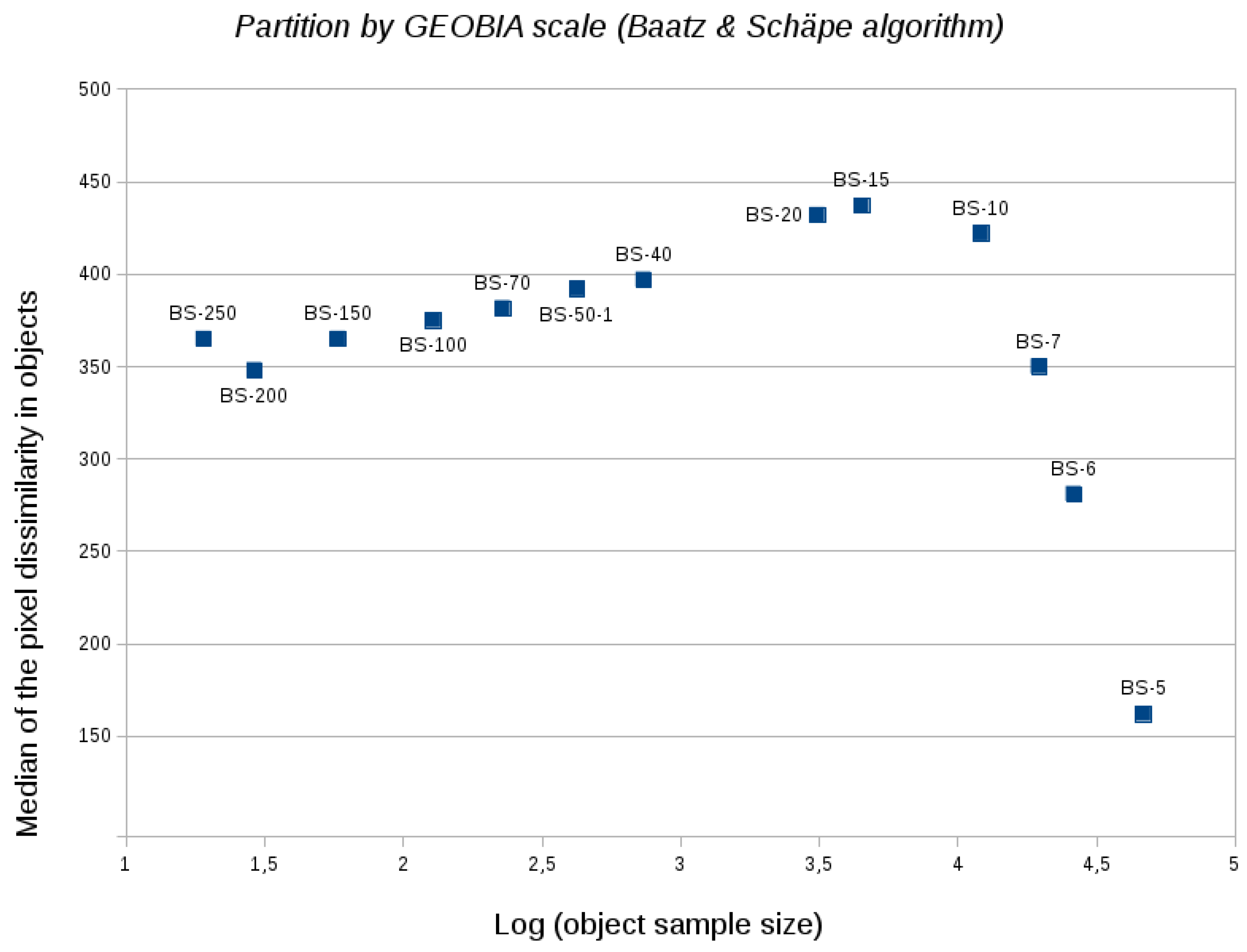
4.4. Some Non Monotonic Progressions of Metrics Values According to Scale

Things become more difficult to interpret when looking at the Figure 15, Figure 16, Figure 17, Figure 18, Figure 19 and Figure 20. The relation between the metrics and the object sample size does not follow a monotonic progression. This involves the following variables: homogeneity, dissimilarity and entropy. Those are all related to the Grey Level Cooccurrence Matrices (GLCM) structure and may be sensitive to the pixel value organization within the polygons. This suggests, on the one hand, that using metrics based on GLMC enriches the knowledge exploration and, on the other hand, that there is not always a monotonic relationship between metrics and scale.
For both dissimilarity (cf. Figure 18 and Figure 19) and entropy from a GEOBIA delineating (cf. Figure 20), there seems to be a peak that was already recurrently observed in previous works about Shannon’s entropy [11]. In this particular case of segmentation, there is a slope inversion between 3.5 and 4 in log, which corresponds to about [3000–15000] polygons. This observation leads to identify a specific scale which maximizes certain metrics. For instance, dissimilarity and entropy show how heterogeneous are the sets of pixels within the objects. We feel, but it is not easy to demonstrate it, that at this peak scale, the objects appear homogeneous compared to each other, although they are composed of various pixels. It may be a kind of regular (or even homogeneous) heterogeneity.

4.5. Some Cases Where GEOBIA Fails in Finding Better Homogeneous Objects

But the previous observation (the peak value) is however not observed for the entropy in the partitions coming from the Baatz and Schäpe algorithm (cf. Figure 20). Moreover, we can see in this plot that the entropy of the segmentations provided by GEOBIA is, in some of the cases, higher than the entropy obtained with grids of similar object size, at comparable scales. This is noticeable in the scales less than 3 in log, that is to say samples with less than 1000 individuals. If entropy is considered as a indicator of homogeneity (since a high entropy shows a high diversity), it suggests that GEOBIA does not provide good results regarding this objective of reducing entropy for a certain range of scale.

5. Conclusions

A first global analysis of the experiments and the values of the different metrics through scales show several main results:
  • For a series of metrics (object compacity, ration perimeter/area, shape index and pixel values amplitude), i.e., all the metrics that do not use GLCM including all the shape measures based on object geometry, we can notice the following results:
    -
    for all the scales, there is a (various) improvement of the object compactness and the pixel values deviation inside objects;
    -
    when the object sample size grows through the scales, the slope of the curve drawn by the metrics values follows the shape curve of the metrics values computed in the grids (with a more or less large deviation); even this deviation sometimes increases (e.g., object compacity and especially shape index).
  • For the rest of the metrics that use GLCM (homogeneity, dissimilarity and entropy):
    -
    it is not possible to check if using GEOBIA algorithms for partitioning is always determinant in improving those metrics; so surprisingly, there does not seem to be a better homogeneity of the objects in the partitions generated by the GEOBIA algorithms compared to a systematic and arbitrary rectilinear partitioning by a grid, if we consider, as assumed in the introduction, that the better the metrics values, the better the objects detection and the spatial partition;
    -
    more precisely, it seems that when there is an improvement, it highly depends on the scale range (e.g., dissimilarity and entropy).
A second level of reflection concerns the question asked: does GEOBIA mitigate the MAUP? The answer must be finely-shaded.
  • On the one hand, mathematically, finding an only example contradicting this conjecture (which is what we have done in this article, even with several cases) is enough to lead to this answer: it is not possible to state in general that GEOBIA segmentation methods mitigate the MAUP, under the assumption that a “better” partitioning is the one that improves the object homogeneity (regarding included pixels).
  • On the other hand, we observed that in many cases and for several metrics, especially the ones describing the object shape and compactness (compacity, ratio perimeter/area), using GEOBIA algorithms improved the results. So these approaches are useful, if you consider that getting less coarse and more compact objects helps to make “better” maps, by improving maps readability.
  • Moreover, GEOBIA being often seen as an exploratory tool to design a “good” map to delineate and represent spatial objects, we showed that, for some metrics (homogeneity, dissimilarity and entropy), it can be used somehow to look for a (the?) pertinent scale.
So should the spatial analysts previously study with care the robustness of the metrics. For instance, entropy is known as very sensitive to the number of classes and so to the sample size. Moreover, any significant object with a strong meaning may not be statistically homogeneous and may be composed of various features, on which scale has a strong impact. As a matter of fact, MAUP is not only a question of object meaningfulness for a given observed phenomenon that could (should?) be fixed by experts in spatial analysis. It is also a low level (re)sampling problem related to pixels variance in each object and variance between those objects. Because scale is one of the key dimensions in delineating spatial objects, results obtained from GEOBIA, such as from any clustering processes, can be biased by the MAUP, and beyond, by any problem related to change of scale. GEOBIA is a rich, efficient and fruitful way to handle objects by grouping pixels using specific objectives and metrics, but it is unfortunately subject to all the facets of the MAUP in downscaling and upscaling processes. It is then of major importance to handle aggregated spatial data with a particular caution regarding this hidden and impairing effect on spatial statistics.

Author Contributions

Romain Louvet was a PhD student working in Avignon University. He participated in writing the introduction and the state of the art of the paper.

Conflicts of Interest

The authors declare no conflict of interest.

References

  1. Openshaw, S. The Modifiable Areal Unit Problem; Geo Books: Norwich, UK, 1984. [Google Scholar]
  2. Quattrochi, D.A.; Goodchild, M.F. (Eds.) Scale in Remote Sensing and GIS; CRC Press: Boca Raton, FL, USA, 1996. [Google Scholar]
  3. Sanders, L. Models in Spatial Analysis; ISTE, Hermes Science-Lavoisier: London, UK, 2007. [Google Scholar]
  4. Royle, J.A.; Dorazio, R.M. Hierarchical Modeling and Inference in Ecology. The Analysis of Data From Populations, Metapopulations and Communities; Elsevier: Amsterdam, The Netherlands, 2008. [Google Scholar]
  5. Beliakov, G.; Pradera, A.; Calvo, T. Aggregation Functions: A Guide for Practitioners; Studies in Fuzziness and Soft Computing; Springer: Berlin/Heidelberg, Germany; New York, NY, USA, 2007; Volume 221. [Google Scholar]
  6. Wong, D. The Modifiable Areal Unit Problem (MAUP). In WorldMinds: Geographical Perspectives on 100 Problems; Kluwer Academic Publisher: Dordrecht, The Netherlands, 2004; pp. 571–575. [Google Scholar]
  7. Robinson, W. Ecological correlations and the behaviour of individuals. Am. Sociol. Rev. 1950, 15, 351–357. [Google Scholar] [CrossRef]
  8. Langbein, L.I.; Lichtman, A.J. Ecological Inference; Quantitative Applications in the Social Science; SAGE: Beverly Hills, CA, USA; London, UK, 1978. [Google Scholar]
  9. Pearl, J. Causality: Models, Reasoning and Inference, 2nd ed.; Cambridge University Press: New York, NY, USA, 2009. [Google Scholar]
  10. King, G.; Rosen, O.; Tanner, A.M. (Eds.) Ecological Inference. New Methodological Strategies; Cambridge University Press: Cambridge, UK, 2004. [Google Scholar]
  11. Josselin, D.; Mahfoud, I.; Fady, B. Impact of a Change of Support on the Assessment of Biodiversity with Shannon Entropy. In Headway in Spatial Data Handling; SDH’2008, Paris; Springer: Berlin/Heidelberg, Germany, 2008; pp. 109–131. [Google Scholar]
  12. Bierkens, M.F.; Finke, P.A.; de Willingen, P. (Eds.) Upscaling and Downscaling in Plant and Soil Science; Kluwer Academic Publisher: Dordrecht, The Netherlands; Boston, MA, USA; London, UK, 2000. [Google Scholar]
  13. Gehlke, C.; Biehl, H. Certain effects of Grouping upon the Size of the Correlation Coefficient in Census Tract Material. J. Am. Stat. Assoc. 1934, 29, 169–170. [Google Scholar]
  14. Yule, G.U. An Introduction to the Theory of Statistics; Charles Griffin and Cies: London, UK, 1911. [Google Scholar]
  15. Swift, A.; Liu, L.; Uber, J. Reducing MAUP bias of correlation statistics between water quality and GI illness. Comput. Environ. Urban Syst. 2008, 32, 134–148. [Google Scholar] [CrossRef]
  16. Arsenault, J.; Michel, P.; Berke, O.; Ravel, A.; Gosselin, P. How to choose geographical units in ecological studies: Proposal and application to campylobacteriosis. Spat. Spatio-Temp. Epidemiol. 2013, 7, 11–24. [Google Scholar] [CrossRef] [PubMed]
  17. Robinson, A. The Necessity of Weighting Values in Correlation Analysis of Areal Data. Ann. Assoc. Am. Geogr. 1956, 46, 233–236. [Google Scholar] [CrossRef]
  18. Charleux, L. GWR, MAUP et lissage par potentiels. Rev. Int. Géomatiq. 2005, 15-2, 195–209. [Google Scholar] [CrossRef]
  19. Holt, D.; Steel, D.; Tranmer, M.; Wrigley, N. Aggregation and Ecological Effects in Geographically Based Data. Geogr. Anal. 1996, 28, 244–261. [Google Scholar] [CrossRef]
  20. Steel, D.; Holt, D. Rules for Random Aggregation. Environ. Plan. A 1996, 28, 957–978. [Google Scholar] [CrossRef]
  21. Tranmer, M.; Steel, D. Using Census Data to Investigate the Causes of the Ecological Fallacy. Environ. Plan. A 1998, 30, 817–831. [Google Scholar] [CrossRef] [PubMed]
  22. Marceau, D.J.; Gratton, D.J.; Fournier, R.A.; Fortin, J.P. Remote Sensing and the Measurement of Geographical Entities in a Forested Environment. 2. The Optimal Spatial Resolution. Remote Sens. Environ. 1994, 49, 105–117. [Google Scholar] [CrossRef]
  23. Marceau, D.J.; Hay, G. Remote sensing contributions to the scale issue. Can. J. Remote Sens. 1999, 25, 357–366. [Google Scholar] [CrossRef]
  24. Mahfoud, I.; Josselin, D.; Fady, B. Sensibilité des indices de diversité à l’agrégation. Rev. Int. Géomatiq. 2007, 17, 293–308. [Google Scholar] [CrossRef]
  25. Josselin, D.; Mahfoud, I.; Fady, B. Analyse exploratoire des effets de support spatial et de robustesse stattistique sur la fiabilité de la mesure de la (bio)diversité. Photo-Interpr. Eur. J. Appl. Remote Sens. 2009, 1, 1–10. [Google Scholar]
  26. Openshaw, S.; Taylor, P. A Million or so Correlation Coefficients: Three Experiments on the Modifiable Areal Unit Problem; Statistical Applications in the Spatial Sciences; Pion: London, UK, 1979; pp. 127–144. [Google Scholar]
  27. Hui, C. A Bayesian Solution to the Modifiable Areal Unit Problem. In Foundations of Computational Intelligence; Studies in Computational Intelligence; Springer: Berlin/Heidelberg, Germany, 2009; Volume 2, pp. 175–196. [Google Scholar]
  28. Louvet, R.; Josselin, D.; Genre-Grandpierre, C.; Ayal, J. Impact des niveaux d’échelle sur l’étude des feux de forêts du sud-est de la France. Rev. Int. Géomatiq. 2016, 26, 445–466. [Google Scholar] [CrossRef]
  29. Blaschke, T.; Lang, S.; Hay, G.J. (Eds.) Object-Based Image Analysis. Spatial Concepts for Knowledge-Driven Remote Sensing Applications; Lecture Notes in Geoinformation and Cartography; Springer: Berlin, Germany, 2008. [Google Scholar]
  30. Castilla, G.; Hay, G. Geographical Object-Bassed Image Analysis (GEOBIA): A new name for a new discipline. In Object-Based Image Analysis. Spatial Concepts for Knowledge-Driven Remote Sensing Applications; Lecture Notes in Geoinformation and Cartography; Springer: Berlin, Germany, 2008; pp. 75–89. [Google Scholar]
  31. Blaschke, T. Object based image analysis for remote sensing. ISPRS J. Photogramm. Remote Sens. 2010, 65, 2–16. [Google Scholar] [CrossRef]
  32. Blaschke, T.; Hay, G.; Kelly, M.; Lang, S.; Hofmann, P.; Addink, E.; Queiroz Feitosa, R.; van der Meer, F.; van der Werff, H.; van Coillie, F.; et al. Geographical Object-Based Image Analysis—Towards a new paradigm. ISPRS J. Photogramm. Remote Sens. 2014, 87, 180–191. [Google Scholar] [CrossRef] [PubMed]
  33. Lang, S. Object-based image analysis for remote sensing applications: Modeling reality—Dealing with complexity. In Object-Based Image Analysis. Spatial Concepts for Knowledge-Driven Remote Sensing Applications; Lecture Notes in Geoinformation and Cartography; Springer: Berlin, Germany, 2008; pp. 3–27. [Google Scholar]
  34. Hay, G.; Castilla, G. Image objects and geographic objects. In Object-Based Image Analysis. Spatial Concepts for Knowledge-Driven Remote Sensing Applications; Lecture Notes in Geoinformation and Cartography; Springer: Berlin, Germany, 2008; pp. 91–110. [Google Scholar]
  35. Aryal, J.; Josselin, D. Environmental Object Recognition in a Natural Image: An Experimental Approach Using Geographic Object Based Image Analysis (GEOBIA). Int. J. Agric. Environ. Syst. 2014, 5, 1–18. [Google Scholar] [CrossRef]
  36. Korting, T.S. GEODMA: A Toolbox Integrating Data—Mining with Object-Based and Multi-Temporal Analysis of Satellite Remotely Sensed Imagery; INPE: Sao Jose dos Campos, Brazil, 2012. [Google Scholar]
  37. Baatz, M.; Schäpe, A. Multiresolution Segmentation—An Optimization Approach for High Quality Multi-Scale Image Segmentation. In Proceedings of the Angewandte Geographische Informations Verarbeitung XII; AGIT: Salzburg, Austria, 2000; pp. 12–23. [Google Scholar]
  38. Korting, T.S.; Garcia Fonseca, L.M.; Bacao, F.L. Expectation-Maximization x Self-Organizing Maps for Image Classification. In Proceedings of the 2008 IEEE International Conference on Signal Image Technology and Internet Based Systems, Bali, Indonesia, 30 November–3 December 2008. [Google Scholar]
  39. Korting, T.S.; Fonseca Garcia, L.M.; Câmara, G. A geographical approach to Self-Organizing Maps algorithm applied to image segmentation. In International Conference on Advanced Concepts for Intelligent Vision Systems; Blanc-Talon, J., Ed.; Springer: Berlin/Heidelberg, Germany, 2011; pp. 162–170. [Google Scholar]
  40. Haralick, R.M.; Shanmugam, K.; Dinstein, I. Statistical and Structural Approach to Texture. IEEE Trans. Syst. Man Cybern. 1973, 3, 610–621. [Google Scholar] [CrossRef]
  41. Patton, D.R. A Diversity Index for Quantifying Habitat “Edge”. Wildl. Soc. Bull. 1975, 3, 171–173. [Google Scholar]
Figure 1. Around the Modifiable Areal Unit Problem [28].
Ijgi 08 00156 g001
Figure 2. Aerial photography of the Mont Ventoux (southern France).
Ijgi 08 00156 g002
Figure 3. Partition by a grid 16 × 16 with rectangular polygons (GRID-16).
Ijgi 08 00156 g003
Figure 4. Segmentation obtained using Baatz and Schäpe algorithm with scale 70 (BS-70).
Ijgi 08 00156 g004
Figure 5. Segmentation obtained using Baatz and Schäpe algorithm with scale 20 (BS-20).
Ijgi 08 00156 g005
Figure 6. Segmentation obtained using Self Organizing Map (SOM-2-2-15) with the following parameters: radius = 2, alpha = 2 and K = 15 [39].
Ijgi 08 00156 g006
Figure 7. Median of the pixel value maximum amplitude in rectangles; grid 16 × 16 with 256 cells; a quantile classification is used, with the [number of individuals per class].
Ijgi 08 00156 g007
Figure 8. Median of the object compacity; segmentation with Baatz and Schäpe algorithm, at scale 20 providing 228 objects; a quantile classification is used, with the [number of individuals per class].
Ijgi 08 00156 g008
Figure 9. Median of the object shape index; segmentation with Baatz and Schäpe algorithm, at scale 70, providing 3115 objects; a classification with same class amplitude is used, with the [number of individuals per class].
Ijgi 08 00156 g009
Figure 10. Median of the pixel value maximum amplitude in objects; segmentation using a Self Organizing Map processing, providing 3185 objects; a quantile classification is used with the [number of individuals per class].
Ijgi 08 00156 g010
Figure 11. Median of the object compacity.
Ijgi 08 00156 g011
Figure 12. Ratio Perimeter/Area of objects.
Ijgi 08 00156 g012
Figure 13. Median of the object compacity with the segmentation based on GEOBIA.
Ijgi 08 00156 g013
Figure 14. Median of the pixel value amplitude in objects.
Ijgi 08 00156 g014
Figure 15. Median of the pixel value homogeneity in objects.
Ijgi 08 00156 g015
Figure 16. Median of the pixel value dissimilarity in objects.
Ijgi 08 00156 g016
Figure 17. Log(Median) of the object shape index. The grid shape index is not represented because they are constant and equal to 0 in the Y axis.
Ijgi 08 00156 g017
Figure 18. Median of the pixel value dissimilarity in objects with the partition using a grid.
Ijgi 08 00156 g018
Figure 19. Median of the pixel value dissimilarity in objects with the segmentation based on GEOBIA.
Ijgi 08 00156 g019
Figure 20. Mean of the pixel value entropy in objects.
Ijgi 08 00156 g020
Table 1. Metrics used for the experiments; GLCM: Grey Level Cooccurrence Matrices.
MetricsEntitiesMeasureRequirement
HomogeneityPixelsVariabilityGLCM
DissimilarityPixelsVariabilityGLCM
Shannon entropyPixelsInformationGLCM
AmplitudePixelsDeviationStatistical distribution
CompacityObjectShapePolygon geometry
Perimeter/AreaObjectShapePolygon geometry
Landscape Shape IndexObjectPatch complexityPolygon geometry

