Data-driven Bicycle Network Analysis Based on Traditional Counting Methods and GPS Traces from Smartphone


DICAM- University of Bologna, Viale Risorgimento 2, 40136 Bologna, Italy
*
Author to whom correspondence should be addressed.
ISPRS Int. J. Geo-Inf. 2019, 8(8), 322; https://doi.org/10.3390/ijgi8080322
Submission received: 4 June 2019
/
Revised: 2 July 2019
/
Accepted: 24 July 2019
/
Published: 25 July 2019
(This article belongs to the Special Issue Spatial Big Data, BIM and advanced GIS for Smart Transformation: City, Infrastructure and Construction)
Abstract
:This research describes numerical methods to analyze the absolute transport demand of cyclists and to quantify the road network weaknesses of a city with the aim to identify infrastructure improvements in favor of cyclists. The methods are based on a combination of bicycle counts and map-matched GPS traces. The methods are demonstrated with data from the city of Bologna, Italy: approximately 27,500 GPS traces from cyclists were recorded over a period of one month on a volunteer basis using a smartphone application. One method estimates absolute, city-wide bicycle flows by scaling map-matched bicycle flows of the entire network to manual and instrumental bicycle counts at the main bikeways of the city. As there is a fairly high correlation between the two sources of flow data, the absolute bike-flows of the entire network have been correctly estimated. Another method describes a novel, total deviation metric per link which quantifies for each network edge the total deviation generated for cyclists in terms of extra distances traveled with respect to the shortest possible route. The deviations are accepted by cyclists either to avoid unpleasant road attributes along the shortest route or to experience more favorable road attributes along the chosen route. The total deviation metric indicates to the planner which road links are contributing most to the total deviation of all cyclists. In this way, repellant and attractive road attributes for cyclists can be identified. This is why the total deviation metric is of practical help to prioritize bike infrastructure construction on individual road network links. Finally, the map-matched traces allow the calibration of a discrete choice model between two route alternatives, considering distance, share of exclusive bikeway, and share of low-priority roads.
1. Introduction
In recent years, due to congestion, air pollution, climate change, energy scarcity, and physical inactivity, an increasing importance has been attributed to sustainable transport modes, and in particular to cycling. Municipalities have drawn attention to these issues and started to implement different strategies to encourage a greater usage of bicycles on urban streets and to reduce car trips. Many cities have decided to invest in the construction of quality bikeways with the intention to incentivize people to cycle even medium (and long) distances on a daily basis.
Several studies have found positive correlations between bike facilities and levels of bicycling. Dill and Carr [1] have analyzed data from 35 large cities across the U.S., finding that cities with higher levels of bicycle infrastructure were characterized by higher levels of bicycle commuting. Pucher and Buehler found that the key to achieving high levels of cycling in Dutch, Danish, and German cities appears to be the provision of separate cycling facilities [2].
Many researchers have studied cyclists’ preferences and have estimated route choice models for planning new bicycle infrastructure. Most of these studies were based on stated preference (SP) data and on opinion surveys. Dill and Voros [3] explored the relationships between levels of cycling and demographics, objective environmental factors, perceptions of the environment, and attitudes based on the results from a random phone survey of adults in the Portland, Oregon. Stinson and Bhat [4], proposed empirical models to evaluate the importance of factors (such as travel time and pavement quality) affecting commuter bicyclists’ route choices. Winters et al. [5] evaluated 73 motivators and deterrents of cycling based on a survey (telephone interviews) and a self-administered survey (either via the web or mail) of 1402 current and potential cyclists in metropolitan Vancouver. These studies highlighted the cyclists’ preference for physically separated bike paths and on-road bike lanes separated by markers. The known limitation of SP studies arises from the difference between stated and observed behavior [6].
In the past, only a few studies were based on revealed preference (RP) data due to the limited availability of this data type. The results of Howard and Burns [7] show that bicycle commuters in metropolitan Phoenix respond to the provision of bicycle facilities. Nelson and Allen [8] found that each additional mile of bikeway per 100,000 people is associated with a 0.069% increase in bicycle commuting.
Data on cycling volumes is the result of choices actually made by cyclists in a real outdoor environment and therefore help to support decision making. Such information is necessary to understand what factors influence ridership. Bike flows can be collected with traditional manual or instrumental counts, which have some drawbacks: Traditional manual counts lack spatial detail and temporal coverage [9,10]. Instrumental and permanent counting stations do provide continuous data, but cover typically only a small number of road sections [11].
More recently, the widespread use of smartphones and mobile applications for self-localization and navigation has increased the availability of observed cyclists’ data in the form of time series of GPS points, called GPS traces. This type of data provides detailed information about the origin/destination of trips as well as the chosen routes. Furthermore, GPS traces allow to determine the total deviation (detour) generated for cyclists in terms of extra distances traveled with respect to the shortest possible route. Empirical data on detour rates do exist. Detours have been calculated in different ways, see for example Pritchard et al. [12] and Griffin and Jiao [13].
The availability of GPS traces led to the development of new cyclists’ route choice models. Dill collected data on bicycling behavior from 166 regular cyclists (1955 trips) in the Portland, Oregon, using GPS devices [14]. This study highlighted that a well-connected network of low traffic streets may be more effective than adding bike lanes on major streets with a high volumes of motor vehicle traffic. Menghini et al. estimated the route choice model for bicyclists from a large sample of GPS observations (2498 trips) collected in Zürich, Switzerland [15]. Their conclusion has been that the trip-length dominates the choices of the Zurich cyclists. Hood et al. analyzed GPS traces from cyclists (366 users and 2777 trips) in San Francisco, USA, and proved a preference for separated bicycle lanes—especially for infrequent cyclists [16]. Broach et al. estimated the route choice of cyclists (164 users and 1449 trips) in Portland metropolitan area, USA [17]. Their study confirmed that route length and slopes do have a negative effect on cyclists’ route choice. In addition, they found that high traffic volumes, high turn frequencies, and traffic signals are also repellant road attributes according to the cyclists’ route choice. Zimmermann et al. estimated a link-based bike route choice model from a sample of GPS observations (103 users and 648 trips) in the city of Eugene, Oregon [18]. Their study confirmed the sensibility of cyclists to distance, traffic volume, slopes, crossings and the presence of bike facilities, distinguishing between average slope above or below 4%, and traffic volume above or below 8000 vehicles per day. More recently, Bernardi et al. analyzed the GPS traces recorded by approximately 280 bicycle users throughout the Netherlands [19]; the results show a high usage of cycleway links and the preference of the shortest route by frequent cyclists. Casello and Usyukov used GPS data on cyclists’ activities to estimate a generalized-cost function that reflects the cyclists’ evaluation of path alternatives [20]: their model correctly predicted the revealed path choice for 65% of the examined trips.
One of the main problems with GPS data is its representativeness, because data collection is usually provided on a volunteer basis, which is not necessarily representative for the entire population [21]. This type of problem has been highlighted by Jestico et al. [22], who used data provided by strava.com to quantify how well crowdsourced fitness app data represent ridership through a comparison with manual cycling counts in Victoria, British Columbia. Another problem is the level of detail of the network: in many cases, the success of identifying the correct network links from GPS points is limited if the bike network model is not sufficiently detailed [23,24].
This paper explains how to estimate the city-wide bicycle flows and how to identify weak points of the road network in terms of bicycle friendliness. Both methods are data driven, explicit and do not require the calibration of sophisticated models. Nevertheless, a route choice model is also calibrated explaining the reasons for deviations at certain road links.
The paper is organized as follows. Section 2 describes the study area and the features of the bike network. Section 3 depicts the bicycle flows obtained by traditional (manual and instrumental) counting methods and by GPS data collected by smartphone application. Section 3 identifies a correlation between cycling counts and GPS data and describes the bicycle flow reconstruction method. In Section 4, a deviation analysis is carried out and a Logit model is calibrated in order to shed more light on the reasons for the decision of individuals to accept deviations by assessing the route characteristics of chosen routes and shortest routes. Section 5 discusses the results of the analysis. Concluding remarks and future research directions are presented in Section 6.
2. Dataset Description
2.1. Study Area
Bologna is a northern Italian city with approximately 390,000 inhabitants [25]. The climate is convenient for cycling all year, with an annual average temperature slightly below 15 °C and low rainfall (about 700 mm rain/year and 74 days of rain per year). Figure 1 shows an overview map to facilitate the location of the city of Bologna, including a zoom on the city center (see box in Figure 1 bottom left).
The home-to-work bicycle mode share was 8.2% in 2011 [26], which is relatively high compared with other medium to large Italian cities [27]. Nevertheless, the car ownership equals 0.515 cars per inhabitant [25], which corresponds to 0.97 cars per household. Based on a survey carried out by TNS opinion & social network in the 28 member states of the European Union between the 11th and 20th of October 2014, the average bicycle mode share was 8.0% [28], whereas in Italy the percentage of people who frequently commute by bike was approximately 4.7% in 2017 [27]. In addition, all major Italian municipalities show an average car ownership of 0.616 per person and a motorcycle ownership of 0.132 per person [29].
2.2. Bicycle Network
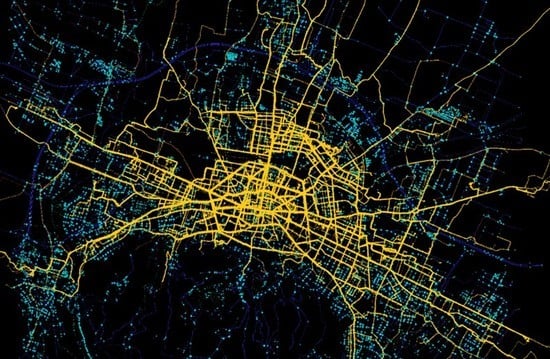
The municipality of Bologna has made substantial investments in bikeways during the past decade and to date the city offers 129 km bikeways of different types: exclusive access and mixed access with pedestrians or buses [25]. The bicycle network layout is composed of 13 main radial bicycle paths connecting the suburbs to the city center and many other bikeways connecting the radial bike-paths. The bikeway meters per citizen increased by 45% starting with 0.228 m/citizen in the year 2009 and reaching 0.330 m/citizen in 2018 [25]. This is an almost linearly-increasing expansion of the cycling infrastructure. The bike-network map is illustrated in Figure 2.
3. Bicycle Flow Analysis
3.1. Cyclists’ Flows from Traditional Counting Methods
During the period 2009–2018, manual and instrumental counts of cyclists were carried out by DICAM-Transport of the University of Bologna [30]: the bicycle counts were conducted from September to October of each year within the study area as shown in Figure 2. In recent years, counting has also been performed in May with the aim to evaluate the difference in bicycle flows between different periods of the same year. The locations of bicycle counters have been selected adopting representative and targeted locations: the sites include different geographic areas of the city, different types of bikeways, as well as “pinch points” (i.e., locations where cyclists must converge to cross a barrier) [10]. The 46 (bidirectional) road-sections monitored in 2018 are showed in Figure 3, highlighting the spatial distribution of measurement points. The monitored road-sections included the 13 main radial bicycle paths. Figure 3 also includes images of different typical bikeway types in Bologna.
Manual and instrumental counting was conducted at each road section from 08:30 to 10:30 on weekdays. The trips purpose during this time period is most likely commute trips for the purpose of “work” or “study”. It is further assumed that commute trips have a clear destination, with a low occurrence of round-trips or random trips for recreational purposes. The total average flows increased between 2009 and 2018 by approximately 75%, which is significantly greater than the increase in bikeway meters per inhabitant in the same period.
Figure 4 shows the correlation between bikeway meters per inhabitant and the total average bicycle flows: each point represents one year from 2009 to 2018.
As shown in Figure 4, the total average bike flows are positively and highly correlated with the length of cycleways per inhabitant (R2 = 0.96). In the city of Bologna, people use bicycles more often than in the past. Surely, such an increase in cycling is determined, like in other cities, by an integrated package of many different and complementary measures, including infrastructure provision, pro-bicycle programs, supportive land-use planning and restrictions of car use [2]. However, today’s bicycle network of Bologna connects the most popular origins and destinations, and the expansion of the cycling network has resulted in an increased level of safety as demonstrated by accident statistics [25]. The increasing bicycle use is also related to an increasing bicycle use of females, growing from a share of below 30% in 2009 to a share of 44% in 2018 [30].
Using the regression function from Figure 4, one can estimate that one additional centimeter of bikeway per inhabitant increases the average bicycle flow by approximately 100 cyclists per hour on the main sections of Bologna’s bicycle network. Based on the length increase of the bicycle network, the estimated bicycle mode share is currently almost 10%, following the model proposed by Schweizer and Rupi [31]: their model describes the significant linear relationship between meters of cycling infrastructure per inhabitant and bike mode share (R2 = 0.81), based on approximately 9000 questionnaires carried out in 14 cities in Central Europe.
3.2. Map Matched Cyclists’ Volumes
A database with GPS traces has been obtained from a data collection initiative called the “European Cycling Challenge” (ECC) [32] which took place in May 2016. In particular, the city of Bologna participated in this initiative among other 51 cities from 18 European countries. In Bologna, 1123 participants, equal to 0.3% of the population, recorded the GPS traces of their bicycle trips during the month of May 2016 by means of a mobile phone application. Participation was on a voluntary basis. The total distance travelled by all participating cyclists was almost 200,000 km and the database contains over 7,998,000 GPS points, with 27,348 individual trips covering the entire road network of Bologna [32] (see Figure 5). There is an area in the southern part of Bologna (encircled in green on Figure 5), with a particularly low density of GPS points, most likely due to the mountains and gardens with bike paths in which the observed bicyclist activity is almost completely absent.
The present analysis focuses only on morning trips from 08:30 to 10:30 during work-days in order to be compatible with the manual and instrumental bicycle counts. During this period, 847 trips were recorded, of which 42% were female and the average age was 38 years. The share of trips carried out by workers with respect to students and the users’ gender are very similar to the last trips census survey of Bologna [33]. However, the census is referred to the active people that use all means of transport. In addition, the share of GPS traces recorded by females is very similar to the share of females observed during the manual counts. Consequently, the sample of cyclists recording the GPS traces is representative of the gender of the counted cyclists. Unfortunately, the ECC database contains no information concerning trip purposes.
In order to obtain bicycle flows on network links, the GPS data has been matched to the road-network based on open street map (OSM). The OSM data has been extracted for the Bologna metropolitan area and converted into a SUMO (Simulation of Urban Mobility) network [34] using a software extension called SUMOPy [35] as reported in Rupi and Schweizer [23]. The SUMO network has been manually corrected and enhanced, such that cyclists could potentially pass everywhere, including footpaths and the opposite direction of one-way roads (which is an illegal behavior in Italy). The final network contains 13,959 nodes and 38,324 links. The employed map matching algorithm is part of SUMOPy and based on a method proposed by Marchal et al. [36] and improved by Schweizer et al. [37]. In order to match the GPS points to network links with a high accuracy and to obtain a large number of correctly matched GPS traces, the entire map-matching analysis consists of four phases [23]: (i) an initial filtering process, (ii) the actual map matching process, (iii) a post-filtering process, and (iv) a final analysis of the matched routes. Initially, many GPS traces could not be matched to the network due to missing links or missing access. Successively, the reasons for the failed matching of trips have been analyzed in detail and missing network links or road access attributes have been added. Finally, the map-matching process has been repeated with an increased number of successfully matched trips.
After the map-matching process and a filtering process ensuring a low error rate, 4029 map-matched routes, collected from 842 users, have been used. These traces correspond to 91.6% of all traces recorded during the considered morning period. It is worth mentioning that this percentage is significantly higher than that reported in other studies [23,24]. Starting from these map-matched routes, the bicycle flows (as the number of cyclists passing through each network link per hour) have been evaluated.
3.3. Estimated Cyclists’ Volumes
A linear regression between the cyclists counted with traditional methods and the number of map matched GPS traces with links overlapping the monitored road sections has been carried out. The map matched bicycle volumes have been multiplied by a coefficient c in order to minimize the difference between the measured flows and flows derived from GPS data.
The regression, shown in Figure 6, is based on the flow-comparison at 23 monitored sections (c = 0.91).
The slope of the linear regression function is almost equal to one, highlighting that the average of map-matched cyclist volumes are equal to the average of manually counted cyclist volumes.
The relatively high level of correlation between the measured flows and the flows from the map matched GPS traces is evident.
Given the significant correlation between the GPS dataset and traditional counts, the linear relation between both flow types has been used to determine the flows on all network links where GPS points have been detected. The resulting link flows in cyclists per hour per direction are shown in the Figure 7. This map is particularly useful to quantify the spatial distribution of ridership and provide important cycling exposure data for safety studies. Starting from this map, it is possible to obtain the OD matrix of cyclists, the chosen routes, and the bicycle flow on every link of the network. This is essential information for modelling the cyclists’ route choice behavior and for planning the bicycle network.
In addition, Strava provides the cyclist heatmap of all cities in the world for trips using the Strava app. The heatmap is calculated by counting and normalizing the number of lines connecting recorded GPS points [38]. The Strava app collects mainly recreational trips and in particular sport trips. The Strava density heatmap of recorded GPS points in Bologna is reported in Figure 8. This figure highlights how the recorded trips are also spread in the south of Bologna, in mountain routes as well as in gardens provided with bike paths (encircled in green). Instead, ECC’s traces from 8:30 to 10:30 cover the main cycle ways that directly connect different parts of city, but there is an absence of trips in the south part, compared with the encircled area of Figure 5. This is probably due to the difference in trip purposes, supporting the hypothesis that the ECC sample contains few leisure trips.
4. Deviation Analysis
The deviation analysis aims to identify the network links which are the most avoided by all cyclists who registered GPS traces. The analysis starts with the following basic assumption: given the choice of two routes with identical properties (same safety, pavement, environment, etc.), cyclists would always choose the shortest one. If this is true, the cyclist would only accept a longer route if it offered better properties (safer, quieter, etc.). From a different perspective, if certain road links are avoided by deviating on alternative links, then the avoided links are supposed to possess fewer attractive characteristics with respect to the alternative, even though these characteristics may be good in the absolute sense. In an ideal bicycle network, no cyclists should feel constrained to take a longer route due to some repellant characteristics of the shortest route, or due to the better characteristics of longer routes. The most “avoided links” of the city’s road network are therefore identified with the km of deviation caused to cyclists. The total deviation metric for each road link i is calculated in the following way:
- For each matched route of the set of all matched routes J, determine the shortest route connecting the first and last link of each matched route.
- For each matched route , identify all non-overlapping sections where links deviate from the shortest route. Set contains all chosen links of the partial deviation k of route j and set contains all links on the shortest route of deviation k and route j, as illustrated in Figure 9.
- For each of these non-overlapping sections, calculate the partial deviation which is the difference between the length of the part of the chosen route segment and the length of the corresponding part of the shortest route segment ; finally the deviation metrix of link i is the sum of partial deviations of all routes that contain link i on one of the shortest route segments. Analytically, the total deviation metric of a road link i is the sum of all partial deviations received from all non-overlapping sections of all matched trips and can be expressed as:where if contains link i, otherwise 0. Let be the length of link i; then the partial deviation is given by
Figure 9 shows links 1, 2 and 3 which are not chosen, despite they are part of the shortest route (solid line); whereas, links 4, 5 and 6 are part of the chosen route (dashed line). In case of the non-overlapping section between node A and B shown in Figure 9, the chosen route is constituted by links 4, 5 and 6, while the shortest route section contains links 1, 2 and 3. The partial deviation of links in equals to L4 + L5 + L6 − (L1 + L2 + L3). The total deviation metric for the central part of Bologna network is shown in Figure 10.
The highest total deviation metric can been seen on the main radial roads from and into the city center. As seen in Figure 10, these are also roads with high bicycle flows. This means that many cyclists actually do use these radial roads but also many try to avoid them. Note that there are also roads in the city center with high bicycle flows, but generating almost no deviations. For a discussion of these findings, see Section 5.
On average, the chosen route parts are 20% longer with respect to the shortest route parts. Analyzing the road attributes of the chosen part and the shortest part of all non-overlapping sections of all trips, the causes for the deviations become clearer—see the first three columns of Table 1. As expected, cyclists accept deviations in order to travel on roads with: (1) a high share of reserved bikeways, (2) a high share of low priority roads (roads with one lane per direction and speed limits of 30 km/h), (3) a low intersection density, and (4) a low share of mixed access, such as lanes with bike/bus access or lanes where bikes and pedestrians are allowed. This last result confirms the findings of the research carried out by Bernardi et al. [39], in which the authors quantified the effects and frequencies of disturbances on bicycle facilities, particularly from pedestrians and buses.
The statistics of the road link attributes of the overlapping sections of each trip (i.e., all links where the chosen and shortest routes coincide) are presented in the last column of Table 1. It becomes evident that the values of the mixed road access share, the reserved bikeway share and the intersection density are in between the values of the shortest route (column 1) and the chosen route (column 2) of the non-overlapping sections. One could conclude that cyclists tend to deviate if road attribute values are below/above those of the overlapping sections. An exception is the low priority road share, where the overlapping sections show values even below that of the shortest route.
In order to shed more light on the decision of individuals to accept deviations, a Logit model is calibrated, where the user has the choice between two alternatives of non-overlapping route segments (as illustrated in Figure 9), where one of the alternatives is the shortest route. The systematic utility function of alternative i is defined as:
where is the distance of the route segment, is the share of exclusive bikeway, and is the share of low priority roads as percentage of the respective distance. The set of observations has been prepared as follows. In a first subset, the route sections have been considered, where the chosen route is different from the shortest route. In a second subset, route sections have been identified, where the shortest route completely coincides with the chosen route. In this case, a longer route alternative (that has not been chosen by the cyclist) has been generated as follows: the second shortest route that connects the extremities of the shortest route section is determined such that the second shortest route section does not overlap with the shortest route section. This is similar to the method applied by Marchal et al. [36]. In this way, a route alternative is generated that is the closest possible to the chosen (and shortest) route alternative. In order to avoid a bias towards longer or shorter distances, the size of the first and second observation subset are kept equal.
The calibration resuls of a total of 4678 observations is shown in Table 2. The attributes chosen are all significant and R2 = 0.160. The small parameter values result in Odds ratios close to one, which is reasonable considering that attribute values are in the order of 10−2–10−3. Other attributes like the node density or the share of mixed bikeway access have turned out not to be significant when included in this model. The signs of the model parameters are reasonable—see also the discussion in Section 6. The calibration has been repeated with GPS traces in Bologna from the ECC of the year 2015. The result of this calibration shows parameter values within the standard error bounds of the result from ECC of the year 2016 shown in Table 2.
One can use Equation (2) to estimate the deviation necessary to equilibrate the systematic utilities of both route alternatives. Setting , and resolving for the deviation yields in
which is the difference in distance, depending on the difference in exclusive bikeway share and the difference in low priority road share. The deviation obtained from Equation (3) ensures a path choice probability of 50%.
5. Discussion
Regarding the estimation of all bicycle flows on the network, the high agreement of flows from GPS traces and manual/instrumental counts (R2 = 0.73) is significantly better than the results obtained by previous studies, e.g., Jestico et al. [22] obtained an R2 of 0.4 for the a.m. peak period. The reason for this difference is likely due to the more detailed network model of Bologna, representing better the cyclists’ freedom to move on all possible links in both directions. Based on this correlation, one crowdsourced cyclist corresponds in average to 59 cyclists counted with traditional methods, which is consistent with previous findings in [22].
Although crowdsourced cyclists represent a small portion of all cyclists, the flows obtained from the map matched GPS data are consistent with the observed flows on the main sections of the Bologna cycle network. Only a few outliers emerge, most likely due to two potential error sources: (1) the days of data sampling of the two methods do not entirely overlap because the GPS records have been registered during the whole month of May, while the traffic counts have been conducted only for two weeks of the same month; (2) the sampling hours do not exactly overlap either, because the GPS traces are selected by their begin time while the traditional methods count the cyclists actually passing by the road-section during the analyzed time interval.
The applied deviation metric from Section 4 quantifies the total deviations of cyclists generated by single road links, but the metric itself does not identify the reasons for the deviations. However, it becomes evident that those radial roads with high bike flows and high deviations in Figure 10 are characterized by an absence of reserved bike lanes, a high level of bus traffic, often on reserved bus lanes, and a high density of intersections. In contrast, those roads where bicycle flows are high but deviations are low, are characterized by low motorized traffic volumes, a high share of bike lanes and the absence of major bus routes.
Nevertheless, the total deviation metric depends on the presence of alternative routes with respect to the shortest route and their respective road attributes: in case there are no feasible route alternatives to avoid a certain link, then the total deviation metric of the respective link is zero, even though the attributes may be unfavourable. In case the shortest route has favourable link attributes but the alternative has even more favourable link attributes, then the total deviation metric is high despite the good conditions on the shortest route. The former case is the most severe as criticalities of unfavourable roads for cyclists without route alternatives remain undiscovered by the deviation analysis.
The calibration of a binominal logit model allows to determine the choice probability, given the attributes of two non-overlapping route alternatives. The attributes distance, share of exclusive bikeways and share of low-priority roads have been found to be significant. The negative sign of and the positive sign of are expected as a longer distance is a disincentive and the presence of a an exclusive bikeway is an incentive for cyclists. The negative sign of related to the share of low-priority roads seems to contradict the previous analyses where the average route on deviations contains a lower share of low priority roads with respect to routes where shortest and chosen routes overlap. One explanation could be the way the alternative routes are generated: probably the second shortest route between two points does use minor roads which cyclists would typically avoid, or cyclists are simply not aware of such alternatives. The determination of road priorities is a heuristic algorithm derived from OSM attributes such as speed limits, number of lanes and access restrictions. It is possible that some types of low priority roads are in reality not attractive to cyclists. A possibility to avoid such problems would be to consider only alternative routes used by at least one cyclist instead of using the adopted route generation method. Another solution would be to specify a model which quantifies the probability to accept a route by considering only the link attributes of the chosen routes, enhanced by a dummy variable indicating whether the chosen route is also the shortest route. Such a model would definitively avoid the problem of alternative route generation. However, modelling errors could be introduced by ignoring all attributes of alternative routes.
The result from Equation (3) relates the differences in road attributes between two alternative routes with the distance that would compensate those differences. The meaning of this result shall be explained by a simple numerical example: assuming two route alternatives, one with a 100% exclusive bikeway and the other without any bikeway, and both alternatives are without priority roads. In such a case, the first alternative could be 3.2 km longer than the second while still attracting 50% of the cyclists.
6. Conclusions
In this research, the cyclists’ flows obtained by traditional counting methods have been compared with GPS traces from smartphones at the same locations and during the same time period.
Although crowdsourced cyclists represent often a small portion of all cyclists, they do represent well the ridership of Bologna in terms of cyclists’ volumes and gender distribution. This result emerges clearly by comparing traditional counting method with GPS traces, confirming their representativeness of the population. The correlation between cycling counts and GPS data collected by smartphones has been relatively high, with an R2 value of 0.73. This correlation is significantly higher than the results obtained by other studies, most likely due to the more detailed representation of the Bologna network, including footpaths in parks and the possibility to cycle one-way roads in both directions. Due to this high correlation, it has been possible to estimate the absolute bicycle flows on all network links by an appropriate scaling of the map-matched flows. The cyclists’ routes are of great value for the planning of cycling infrastructure and the drafting of cycling policies. The proposed method, which combines bicycle counts at a few main road sections with areas covering GPS traces, can readily be applied in other cities in order to reliably estimate the absolute bike flows of an entire urban area.
GPS data have been further used to determine the total deviation metric, which counts the total deviations that a road link causes to cyclists. The total deviation metric is useful to identify weak links of the cycling network, but it does not identify the reason why certain road links are avoided. However, applying the total deviation metric to the Bologna road network, the highest deviation has been seen on trafficked roads without physically protected bike lanes. Also, roads with reserved bus lanes, which are open for bicycles too, showed high deviation rates. Further analyses of chosen and shortest road sections have shown that cyclists are willing to make deviations when the alternative route provides a high share of reserved bikeways, a high share of low-priority lanes, a low intersection density and a low share of roads with mixed traffic (cyclists with buses and pedestrians). Planners should take the deviation metric into considerations for either bike-path construction or bike-network interventions. Obviously, the total deviation metric does not reveal deviations if there are no alternatives to avoid a certain road link. The map-matched traces allowed to calibrate a discrete choice model between two route alternatives, considering distance, share of exclusive bikeway and share of low-priority roads. A longer distance and a higher share of low-priority roads appear to decrease the choice probability, while a higher share of exclusive bikeways does increase the choice probability, as expected. With the same model, it has been possible to quantify the tolerated deviation length in function of the road attributes.
In future works, the representativeness of the results could be improved by statistically weighting the GPS traces according to different person attributes, such as occupation, gender, or age. The route choice model could be enriched by more significant attributes like traffic light density, junctions with left-turns, or junctions with side-roads entering from the right side. In particular, the low-priority road attribute needs to be further refined. The generation of longer route alternatives could be replaced by actually chosen routes and models using only attributes of the chosen routes shall be tested.
Author Contributions
Study conceptualization, Federico Rupi and Joerg Schweizer; Methodology, Federico Rupi and Joerg Schweizer; Programming and data retrieval, Federico Rupi, Joerg Schweizer and Cristian Poliziani; Formal GIS analysis, Joerg Schweizer and Cristian Poliziani; Writing—review and editing, Federico Rupi, Joerg Schweizer and Cristian Poliziani.
Funding
Open access funding provided by Department of Civil, Chemical, Environmental, and Materials Engineering (DICAM)—University of Bologna.
Acknowledgments
We are grateful to SRM Bologna srl for providing the GPS data of the European Cycling Challenge 2016.
Conflicts of Interest
The authors declare no conflict of interest.
References
- Dill, J.; Carr, T. Bicycle Commuting facilities in major US cities: If you build them commuters will use them—Another look. Transp. Res. Rec. 2003, 1828, 116–123. [Google Scholar] [CrossRef]
- Pucher, J.; Buehler, R. Making cycling irresistible: Lessons from The Netherlands, Denmark and Germany. Transp. Rev. 2008, 28, 495–528. [Google Scholar] [CrossRef]
- Dill, J.; Voros, K. Factors Affecting Bicycling Demand: Initial Survey Findings from the Portland, Oregon, Region. Transp. Res. Rec. 2007, 44, 9–17. [Google Scholar] [CrossRef]
- Stinson, M.; Bhat, C. Commuter Bicyclist Route Choice: Analysis using a Stated Preference Survey. Transp. Res. Rec. 2003, 39, 107–115. [Google Scholar] [CrossRef]
- Winters, M.; Davidson, G.; Kao, D.; Teschke, K. Motivators and deterrents of bicycling: Comparing influences on decisions to ride. Transportation 2011, 38, 153–168. [Google Scholar] [CrossRef]
- Sener, I.N.; Eluru, N.; Bhat, C.R. An analysis of bicycle route choice preferences in Texas, US. Transportation 2009, 36, 511–539. [Google Scholar] [CrossRef] [Green Version]
- Howard, C.; Burns, E.K. Cycling to Work in Phoenix: Route Choice, Travel Behavior, and Commuter Characteristics. Transp. Res. Rec. 2001, 1773, 39–46. [Google Scholar] [CrossRef]
- Nelson, A.C.; Allen, D. If you build them commuters will use them–Association between bicycle facilities and bicycle commuting. Transp. Res. Rec. 1997, 1578, 79–83. [Google Scholar] [CrossRef]
- Niemeier, D.A. Longitudinal Analysis of Bicycle Count Variability: Results and Modeling Implications. J. Transp. Eng. 1996, 122, 200–206. [Google Scholar] [CrossRef]
- Ryus, P.; Ferguson, E.; Laustsen, K.M.; Schneider, R.J.; Proulx, F.R.; Hull, T.; Miranda-Moreno, L. Guidebook on Pedestrian and Bicycle Volume Data Collection; National Cooperative Highway Research Program Report 797; The National Academies Press: Washington, DC, USA, 2014. [Google Scholar]
- Griffin, G.; Nordback, K.; Götschi, T.; Stolz, E.; Kothuri, S. Monitoring bicyclist and pedestrian travel and behavior, current research and practice. Transportation research circular E-C183. 2014. Available online: http://www.trb.org/Publications/Blurbs/170452.aspx (accessed on 31 May 2019).
- Pritchard, R.; Frøyen, Y.K.; Bernhard, S. Bicycle Level of Service for Route Choice—A GIS Evaluation of Four Existing Indicators with Empirical Data. Int. J. Geo-Inf. 2019, 8, 214. [Google Scholar] [CrossRef]
- Griffin, G.P.; Jiao, J. Where does bicycling for health happen? Analyzing volunteered geographic information through place and plexus. J. Transp. Health 2015, 2, 238–247. [Google Scholar] [CrossRef]
- Dill, J. Bicycling for Transportation and Health: The Role of Infrastructure. J. Public Health Policy 2009, 30, 95–110. [Google Scholar] [CrossRef] [PubMed]
- Menghini, G.; Carrasco, N.; Schüssler, N.; Axhausen, K.W. Route choice of cyclists in Zurich. Transp. Res. Part A 2010, 44, 754–765. [Google Scholar] [CrossRef]
- Hood, J.; Sall, E.; Charlton, B. A GPS-based bicycle route choice model for San Francisco, California. Transp. Lett. Int. J. Transp. Res. 2011, 3, 63–75. [Google Scholar] [CrossRef]
- Broach, J.; Dill, J.; Gliebe, J. Where do cyclists ride? A path choice model developed with revealed preference GPS data. Transp. Res. Part A 2012, 46, 1730–1740. [Google Scholar]
- Zimmermann, M.; Mai, T.; Frejinger, E. Bike route choice modeling using GPS data without choice sets of paths. Transp. Res. Part C 2017, 75, 183–196. [Google Scholar] [CrossRef]
- Bernardi, S.; La Paix-Puello, L.; Geurs, K. Modelling route choice of Dutch cyclists using smartphone data. J. Transp. Land Use 2018, 11, 883–900. [Google Scholar] [CrossRef]
- Casello, J.M.; Usyukov, V. Modeling cyclists’ route choice based on GPS data. Transp. Res. Rec. 2014, 2430, 155–161. [Google Scholar] [CrossRef]
- Watkins, K.; Ammanamanchi, R.; LaMondia, V.; Le Dantec, C.A. Comparison of Smartphone-based Cyclists GPS Data Sources. In Proceedings of the Transportation Research Board—95th Annual Meeting, Transportation Research Board of the National Academies, Washington, DC, USA, 10–14 January 2016. [Google Scholar]
- Jestico, B.; Nelson, T.; Winters, M. Mapping ridership using crowdsourced cycling data. J. Transp. Geogr. 2016, 52, 90–97. [Google Scholar] [CrossRef] [Green Version]
- Rupi, F.; Schweizer, J. Evaluating cyclist patterns using GPS data from smartphones. ITE Intell. Trans. Syst. 2018, 12, 279–285. [Google Scholar] [CrossRef]
- Khatri, R.; Cherry, C.R.; Nambisan, S.S.; Han, L.D. Modeling Route Choice of Utilitarian Bikeshare Users with GPS Data. Transp. Res. Rec. 2016, 2587, 141–149. [Google Scholar] [CrossRef] [Green Version]
- Municipality of Bologna, Statistics. Available online: https://www.comune.bologna.it/iperbole/piancont/dati.html (accessed on 1 May 2019).
- ISTAT Statistics. 2011. Available online: https://www.istat.it/it/censimenti-permanenti/censimenti-precedenti/popolazione-e-abitazioni/popolazione-2011 (accessed on 1 May 2019).
- Istat Spostamenti Quotidiani e Nuove Forme di Mobilità. 2018. Available online: istat.it/it/files//2018/11/Report-mobilità-sostenibile.pdf (accessed on 1 May 2019).
- Eurobarometer. Special Eurobarometer 422a, Quality of Transport. 2014. Available online: ec.europa.eu/public_opinion/archives/ebs/ebs_422a_en.pdf (accessed on 1 May 2019).
- Conto Nazionale dei Trasporti. 2018. Available online: http://www.mit.gov.it/comunicazione/news/conto-nazionale/online-il-conto-nazionale-delle-infrastrutture-e-dei-trasporti (accessed on 1 May 2019).
- Municipality of Bologna Rilevamento dei Flussi di Biciclette sulle Principali Piste Ciclabili Presenti nel Territorio del Comune di Bologna. Elaborazione dei Dati Raccolti e Confronto con le Serie Storiche Disponibili. 2018. Available online: www.comune.bologna.it/media/files/report_flussi_ciclabili_2018.pdf (accessed on 1 May 2019).
- Schweizer, J.; Rupi, F. Performance evaluation of extreme bicycle scenarios. Procedia-Soc. Behav. Sci. 2014, 111, 508–517. [Google Scholar] [CrossRef]
- European Cycling Challenge. 2016. Available online: www.europeancyclingchalleg.org (accessed on 1 May 2019).
- Statistical Analysis of Bologna Trips. Available online: https://www.comune.bologna.it/iperbole/piancont/Cens_Pop_2011/pendolarismo/Pendolarismo.pdf (accessed on 1 May 2019).
- Sumopy. Available online: https://sumo.dlr.de/wiki/Contributed/SUMOPy (accessed on 1 May 2019).
- SUMO. Available online: http://sumo.sourceforge.net/userdoc/ (accessed on 1 May 2019).
- Marchal, F.; Hackney, J.K.; Axhausen, K.W. Efficient map matching of large Global Positioning System data sets: Test. on speed-monitoring experiment in Zurich. Transp. Res. Rec. 2005, 1935, 93–100. [Google Scholar] [CrossRef]
- Schweizer, J.; Bernardi, S.; Rupi, F. Map-matching algorithm applied to bicycle global positioning system traces in Bologna. ITE Intell. Transp. Syst. 2016, 10, 244–250. [Google Scholar] [CrossRef]
- Strava Global Heatmap. Available online: https://www.strava.com/heatmap#13.41/11.34182/44.48590/hot/all (accessed on 1 May 2019).
- Bernardi, S.; Krizek, K.J.; Rupi, F. Quantifying the role of disturbances and speeds on separated bicycle facilities. J. Trans. Land Use 2016, 9, 105–119. [Google Scholar] [CrossRef]
Figure 1.
Bologna location in the Italian contest.

Figure 2.
The bike-network map of Bologna [24] and study area (dashed lines).
Figure 2.
The bike-network map of Bologna [24] and study area (dashed lines).

Figure 3.
Road sections monitored in 2018—Legend shows sections sorted by flow value.

Figure 4.
Regression function between length of cycleways per inhabitant and bike flows.

Figure 5.
ECC 2016: observed cyclist activity in the Bologna network.

Figure 6.
Regression function between manually counted cyclists’ volumes and map matched cyclists’ volumes (May 2016).
Figure 6.
Regression function between manually counted cyclists’ volumes and map matched cyclists’ volumes (May 2016).

Figure 7.
Estimated unidirectional bicycle flows in cyclists per hour during workday morning peak hours (from 8:30 to 10:30). Flows only on network links where GPS points have been detected.
Figure 7.
Estimated unidirectional bicycle flows in cyclists per hour during workday morning peak hours (from 8:30 to 10:30). Flows only on network links where GPS points have been detected.

Figure 8.
The Strava heat-map of Bologna.

Figure 9.
Illustration of the calculation of the total deviation metric for the non-overlapping route section between nodes A and B.
Figure 9.
Illustration of the calculation of the total deviation metric for the non-overlapping route section between nodes A and B.

Figure 10.
Total deviation metric determined for the central part of Bologna network.


Table 1.
Road link attributes of chosen and shortest routes of non-overlapping sections and on overlapping sections.
Table 1.
Road link attributes of chosen and shortest routes of non-overlapping sections and on overlapping sections.
| Non-overlapping Sections | Overlapping Sections | |||
|---|---|---|---|---|
| Shortest route | Chosen route | Chosen vs Shortest | Chosen and shortest route | |
| Total length [km] | 8265 | 9975 | +20.7% | 7130 |
| Mixed road access share | 32.6% | 25.7% | −21.2% | 28.4% |
| Low priority road share | 50.0% | 74.1% | +48.2% | 40.2% |
| Reserved bikeway share | 16.4% | 39.2% | +139.0% | 23.5% |
| Intersection density [1/km] | 18.5 | 15.9 | −14.2% | 16.1 |
Table 2.
Calibration results of Logit model from Equation (2).
| Attribute | Parameters | Odds Ratio | Std. err | z | p > |z| |
|---|---|---|---|---|---|
| Distance | −0.0007 | 0.9992 | 9.10 10−5 | −7.4585 | 8.7531 10−14 |
| Reserved bikeway share | 0.0228 | 1.0230 | 8.82 10−4 | 23.1713 | 8.8673 10−119 |
| Low priority road share | −0.0085 | 0.9915 | 6.88 10−4 | −12.0599 | 1.7192 10−33 |
© 2019 by the authors. Licensee MDPI, Basel, Switzerland. This article is an open access article distributed under the terms and conditions of the Creative Commons Attribution (CC BY) license (http://creativecommons.org/licenses/by/4.0/).
Share and Cite
MDPI and ACS Style
Rupi, F.; Poliziani, C.; Schweizer, J. Data-driven Bicycle Network Analysis Based on Traditional Counting Methods and GPS Traces from Smartphone. ISPRS Int. J. Geo-Inf. 2019, 8, 322. https://doi.org/10.3390/ijgi8080322
AMA Style
Rupi F, Poliziani C, Schweizer J. Data-driven Bicycle Network Analysis Based on Traditional Counting Methods and GPS Traces from Smartphone. ISPRS International Journal of Geo-Information. 2019; 8(8):322. https://doi.org/10.3390/ijgi8080322
Chicago/Turabian StyleRupi, Federico, Cristian Poliziani, and Joerg Schweizer. 2019. "Data-driven Bicycle Network Analysis Based on Traditional Counting Methods and GPS Traces from Smartphone" ISPRS International Journal of Geo-Information 8, no. 8: 322. https://doi.org/10.3390/ijgi8080322
Note that from the first issue of 2016, this journal uses article numbers instead of page numbers. See further details here.