Article

An Agent-based Model Simulation of Human Mobility Based on Mobile Phone Data: How Commuting Relates to Congestion

1
Department of Graphics and Digital Technology, School of Urban Design, Wuhan University, Wuhan 430072, China
2
Department of Urban Planning, School of Urban Design, Wuhan University, Wuhan 430072, China
*
Author to whom correspondence should be addressed.
ISPRS Int. J. Geo-Inf. 2019, 8(7), 313; https://doi.org/10.3390/ijgi8070313
Submission received: 5 June 2019 / Revised: 15 July 2019 / Accepted: 20 July 2019 / Published: 23 July 2019

Abstract

:
The commute of residents in a big city often brings tidal traffic pressure or congestions. Understanding the causes behind this phenomenon is of great significance for urban space optimization. Various spatial big data make the fine description of urban residents’ travel behaviors possible, and bring new approaches to related studies. The present study focuses on two aspects: one is to obtain relatively accurate features of commuting behaviors by using mobile phone data, and the other is to simulate commuting behaviors of residents through the agent-based model and inducing backward the causes of congestion. Taking the Baishazhou area of Wuhan, a local area of a mega city in China, as a case study, we simulated the travel behaviors of commuters: the spatial context of the model is set up using the existing urban road network and by dividing the area into space units. Then, using the mobile phone call detail records of a month, statistics of residents’ travel during the four time slots in working day mornings are acquired and then used to generate the Origin-Destination matrix of travels at different time slots, and the data are imported into the model for simulation. Under the preset rules of congestion, the agent-based model can effectively simulate the traffic conditions of each traffic intersection, and can induce backward the causes of traffic congestion using the simulation results and the Origin-Destination matrix. Finally, the model is used for the evaluation of road network optimization, which shows evident effects of the optimizing measures adopted in relieving congestion, and thus also proves the value of this method in urban studies.

1. Introduction

With the expansion of urban scale and the rapid growth of motor vehicles, traffic congestion has become an increasingly serious urban problem, and the tidal traffic generated by the commuting of residents is believed to be one of the major causes of traffic congestion [1,2]. Traffic congestion not only brings energy waste and environmental pollution [3], but is also believed to negatively affect public health [4]. To address this problem, common approaches including economic or policy measures based on econometric models are used, such as congestion pricing [1,5,6,7], encouraging the use of public transport [8,9,10], etc. However, models commonly used in these approaches are static, in which residents’ distribution and mobility in space are seldom considered, thus bringing inaccuracy of results [11]. Currently, increasing the availability and utilization of urban spatial big data, especially location-based service (LBS) data from GPS devices, smart cards, and mobile phones, make it possible to describe urban residents’ travels more accurately on a finer scale [12]. Data of residents’ mobility over time and space can be used for urban geographic mapping [13], epidemiological analysis [14,15], real-time urban monitoring [16], etc. and can also be used for recognition of urban spatial features [17,18,19] or measurement of urban vibrancy [20]. Another important scenario of application is the study of residents’ commuting and urban transport, including the identification of commuting areas and commuting distances [21,22], and the acquisition of commuter Origin-Destination (OD) matrices [23,24,25]. Among various sources of location data, mobile phone data have been widely employed in studies such as residents’ commuting thanks to its extensive coverage, passive data collection, and the fact that its data acquisition requires no extra equipment. In comparison, alternative data sources, such as smart card data or taxi GPS data, have equivalent difficulties in data coverage but much smaller population coverage [26]. Results of studies based on new data have been shown to have higher accuracy compared to those that are based on statistical data or measured data, proving the effectiveness of big data application in urban studies. In general, most of these studies are at an early stage of describing urban phenomena through data, few studies attempt to go further such as using big data to identify the connection between residents’ travel and traffic congestion, or to predict and evaluate measures for traffic improvement [27,28].
After obtaining relatively accurate data for residents’ commuting, modeling and simulation can be an approach to identifying the mechanism and rules behind the functions of urban spaces. The agent-based model (ABM) is considered one of the most effective techniques for simulating complex systems and thus has great advantage to study cities, which are typically complex systems [29]. The distributed characteristics of ABM enable it to reflect differences in the behaviors of different types of individuals [30]. Therefore, the model can be used to simulate traffic flow and residents’ behaviors in urban transport, including the residents’ choice of travel modes [31] and carpooling models [32]. Other research applications are found in the optimization of bus routes [33,34], the simulation of the functioning of the urban composite transportation system [35], the evaluation of the impact of the intercity high-speed railway on the ecological environment [36], etc. From the perspective of development trends in research, studies are moving from the simulation of individual decision-making to that of the composite flow of urban traffic, with increasing complexity of simulation. However, most of these simulations are still based on survey data, which not only are expensive and time-consuming to acquire but also lack details of residents’ travel behaviors. For these reasons, big data are considered to be a better data source for studies of residents’ travel behaviors [37].
Among others, call detail records (CDRs) are commonly employed as a kind of urban spatial big data. Compared with traditional survey data, it has higher sample coverage, time efficiency in acquisition, and higher time resolution [38]. On the other hand, as an effective tool for studying urban spaces, ABM has long been fettered by the lack of data in its earlier developments and it sees great potential in the current context of smart city development [39]. Therefore, using CDRs in ABM offers great promises for traffic simulation that reflects actual urban spatial environment and the spatial distribution of residents. The simulation, in turn, can be used to analyze the causes of traffic congestion and even to predict traffic conditions under different application scenarios. In previous studies, although big data is gradually applied to generate the OD matrix of the residents’ travels and to predict traffic pressure in the actual urban road network, the following weaknesses still exist: first, most of these studies were conducted on a macro scale of the whole city. At such a scale, road capacity is often ignored, despite the fact that it is crucial for relieving traffic congestion; second, most studies presume that all commuting travels begin simultaneous, without addressing the differences in traffic volume in different time periods. Apparently, considerable errors may occur in the prediction of traffic conditions on the micro scale. Therefore, these two points were taken into consideration in the model employed in the present study.

2. Materials and Methods

The present research comprises two major parts: the acquisition of the features of residents’ commuting behavior and simulation of commuting behavior of urban residents.

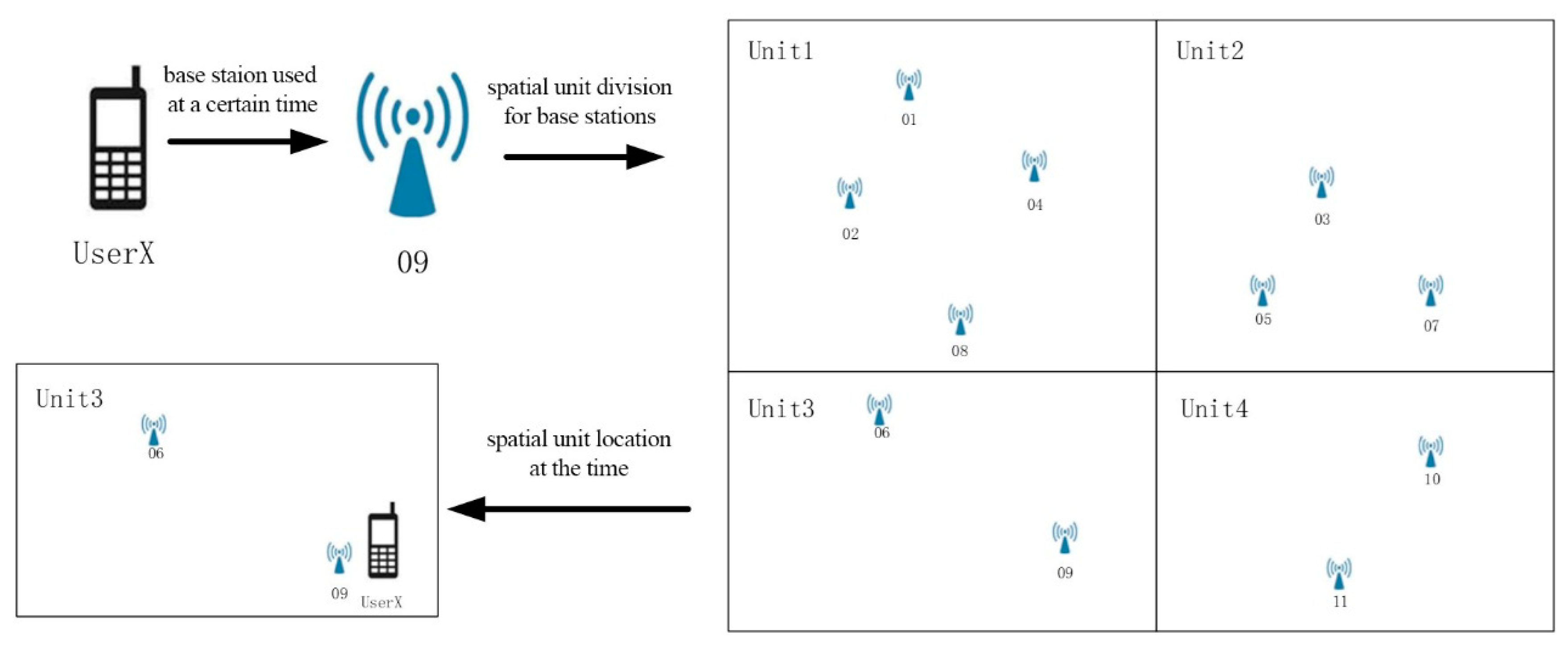
2.1. Mobile Phone Data Processing

As mobile phone data is directly related to the spatial distribution of the base stations, its accuracy in positioning is also determined by the density of base stations and varies across different areas. In addition, due to the different way of work and life of various users, the acquired phone call behavior is also fuzzy data with an uneven distribution over time. In general, mobility studies using mobile phone data usually take areas with densely distributed base stations such as city centers as case studies. User’s location is represented by the location of the base station that has recorded the most frequent phone calls by the user within a specific period (one month or several months) at a specific time (working hours or at an interval of several hours). Subsequently, by associating the locations of various base stations along the timeline, user’s mobility trajectory can be generated using CDR data [17,19,21,23,24,25,38,40,41,42]. The present study uses a similar approach while focusing on the rush hours and dividing the timeline on an hourly basis. Data are processed in combination with the ArcGIS platform, and the raw mobile phone data (Table 1) comprise CDRs of 7 million users in the case city over a time period of one month.
Data processing followed the procedures below:
a. Invalid data and users who make less than three phone calls per month were removed. After the screening, 3.8 million users remained.
b. Users’ CDR data were sorted into working hours (7:00 to 18:00, Monday to Friday) and non-working hours (Saturday and Sunday, and 7pm to 6am on weekdays). Base station locations with the highest call frequency during the two time periods were identified as the place of work and residence, respectively.
c. Frequency of phone calls on working days (Monday to Friday) was calculated based on user’s CDRs every 24 hours, and field value of the base station ID with the highest call frequency during the period was extracted (as shown in Table 2).
d. The four hours from 6:00 to 9:00 were identified as the peak commuting period. Based on space unit division and base station location, base station ID and space unit code were associated (Figure 1). By comparing the codes of space unit and residence location of a user at each hour, the departure time was determined and the base station ID matrix of origin and destination was obtained. (The decision rule is: if a user’s space unit code is 0 at 6:00, and is different from the code of the residence space unit at 7:00, 6:00 is thus decided as the departure time, the code of the residence space unit is decided as the origin, and the code of space unit at 7:00 is decided as the destination. If the code of space unit at 7:00 is still 0, the departure time is further extended to the next time period till the code is not 0 and code of space unit is different from the residence code. If the space unit code at 6:00 is not 0, users with space unit codes at 6:00 and 7:00, 8:00 and 9:00, or 6:00, 7:00, 8:00, 9:00 and 11:00 are searched respectively. Whenever a change in space unit codes occurs, the different units will be decided as the origin and destination. Furthermore, an OD matrix for different hours is generated.)
Subsequently, the OD matrix of residents’ travels in the case area were imported into the ABM as basic data.

2.2. Agent-Based Model

ABM is often used in complex giant systems such as cities. Generally speaking, a Multi-Agent System (MAS) contains many types of agents, including mobile agents such as urban residents and static agents such as urban roads. Agents run by pre-defined rules and interact with one another, producing movement and dynamic changes starting from an individual agent to the whole. As this mechanism resembles the interaction between human individuals, human and space in the city, ABM is considered as one of the best tools to understand urban functioning [43]. The model in the present study is established on the Repast S platform, and the settings of external environment and agent mobility draw reference from the open source model RepastCity [44,45,46]. Since residents’ traveling is the only behavior studies in the research, the modeling of urban environment can be simplified into the spatial units of travel (i.e., origin and destination) as well as urban roads. Agents’ behavior rules mentioned below are coded by Java and added to the RepastCity model to make it run as we designed. The rules for model running are that a resident agent moves from one spatial unit (origin) to another spatial unit (destination) at a specific time point. When the resident agent runs on the road, it may lower its speed of movement due to preset traffic congestion conditions (Figure 2).

2.3. Model Hypothesis and Parameter Setting

The following hypothesis and rules are made regarding the generation of an Agent in the model and its behaviors:
First, each Agent (urban resident) generated has a specific origin and destination of travel, at a specific time point of departure. In the model, all resident Agents are generated simultaneously but are set with a specific delay value each, according to their different departure time. For example, residents depart at 6:00 have a delay value of 0 s, while those who depart at 7:00 have a delay value of 3600 s. In addition, each resident Agent is represented by a private car whose initial speed of travel is based on the driving speed of a normal motor vehicle.
Second, on each plot, a certain number of Agents is generated which is calculated using the number of residents acquired through phone data, then divided by operator’s market share, and finally multiplied by the ratio of motor vehicle travel of residents.
Thirdly, traffic congestion emerges when a certain number of resident Agents concentrate in the same road intersection, and the traveling speed of residents varies in accordance to the level of congestion. Roads and nodes in the mode are generated from a shape file built in ArcGIS and are converted to Agents in RepastCity.
Fourth, residents choose the shortest route to their destination and do not change route before their arrival. The choice of path by Agents is based on the Dijkstra algorithm. Codes of space units as origin and destination are acquired in the OD matrix, and the shortest route is calculated in accordance with the road network and algorithm.
There are three major parameter variables in the commuting travel model of urban residents in the study area:
The first one is the commuter travel data of residents in each plot acquired from the OD travel matrix, and the number of travels of the corresponding Agent. The number of Agents is decided based on two factors: first, the number of residents acquired through phone data is converted to get the number of commuting residents, and is converted to get the number of travels by motor vehicles. As the Baishazhou area is located in the outskirt of the city near the Third Ring road with no subway lines, and the number of bus lines is far less than those in the inner city area, it is assumed that the majority of travels are made by private cars. The number of residents acquired through phone data is divided by the market share of the telecom operator and then the number of private car travels is acquired at a conversion factor of 1 to 1. The second factor is the ratio of the number of Agents in the simulation to the actual number of residents traveling by cars. In the statistics, we observed that there ~15,000 people traveling at the 9–10:00 period when the amount of travels is at the lowest in the study area. Previous test modeling showed that, with increasing number of Agents, the speed of simulation drops significant, while the precision of simulation results does not increase accordingly. Therefore, in the present simulation, the number of Agents is reduced so as to improve the efficiency of simulation and the traffic capacity of roads has been adjusted proportionally. The final resident-to-Agent ratio is set at 1:10, that is, one Agent represents 10 residents.
The second parameter is the speed setting. Considering the hierarchy of roads in the study area, such as urban expressways, artery roads, etc., the Agent’s speed on the roads is also differentiated. In the study, two different speeds are set, i.e., the expressway speed, at 50 km/h and the artery road speed, at 30 km/h. This parameter is achieved by specifying the field of road attribute in GIS, corresponding to the speed parameters of 13.9 m/s and 8.3 m/s, respectively. The speed setting also correlates the Agent’s travelling speed with the actual time unit, that is, each operation cycle (1 tick in simulation) is equal to 1 second of real time.
The third parameter is the road congestion settings. As the present study is conducted on a meso to macro scale area, roads are not categorized on a finer level, nor is the overlapping of vehicles considered. Congestion is defined by the instantaneous density of Agents on the road as vehicle density can directly demonstrate the congestion level on a road and road occupancy is often used as a quantitative indicator in traffic analysis [47]. According to the methods used in previous literature [48], the present study defines road occupancy at 0.5–1 as serious congestion, 0.3–0.5 as slight congestion, and below 0.3 as no congestion.

3. Case Study

This Baishazhou area (Location: 30.42°~30.53° N, 114.25°~114.30° E) in Wuhan was selected as the case study of commuting simulation based on the following considerations: first, Baishazhou is a new area of Wuhan, which is mostly residential in function. Therefore, the study of the impact of commuting on traffic condition in this area is of practical value. Second, since the area is still under construction and development, follow-up observations are possible to identify the differences between the simulation results of various planning programs and the traffic condition in reality. Thus, the proposed optimization and improvement measures may be of great practicality. Finally, as there is a city-level artery road in this area, i.e., the Baishazhou Avenue, the overall urban layout is distributed along the road in a belt-like shape. With frequent and extensive interactions with the surrounding areas and evident concentration of vehicle traffic, the area is deemed a valid case to evaluate the effectiveness of the model.

3.1. Data Acquisition and Processing

After the processing of mobile phone data is completed, the most important step is to allocate the residence and work places of residents at each hour to the space units. This is realized by overlapping aerial photographs, vector electronic map, and existing roads onto previously generated space units. Working with a huge dataset like mobile phone data, the number of time division, and space unit division by different hours of a day may lead to an exponential increase in total statistical size. Therefore, except for the case study area, the division of urban space is minimized to reduce the total number of spatial units. Finally, 34 space units were generated (see Figure 3). Based on these space units, statistics were extracted for the four rush hours on each workday morning. Among these units, plots No. 1 to No. 27 were taken as the core research objects, in which commuting data of residents were acquired. Since the accurate travel routes in other plots cannot be obtained without a fine division, these plots were selected only as destinations but not origins.
Using Monday to Friday every week as the time periods in the present study, temporal features of the residents’ commute were obtained. In regular commuting, residents’ travel from home to work in the morning rush hours and then from work to home during the evening rush hours. In order to reduce the amount of data in space unit division, the division of land for work is simplified. Therefore, only the commuting of residents during the morning rush hours, i.e., the four hours from 6:00–10:00, were considered in the present simulation. Using the base station data in the four hours of 6:00, 7:00, 8:00, and 9:00, the number of plots at 11:00, the number of travels at each hour and at each plot were generated and further generated an OD matrix (Table 3). The number of residents’ travels in each core space unit at different hours separately was acquired (Figure 4). The ranking of the numbers for the four time slots was 7:00 > 8:00 > 6:00 > 9:00, which is consistent with our daily experience: since most employers in China set working hours between 9:00 to 17:00, residents leave home for work between 7:00 to 8:00 to reserve enough time for commuting even in face of the possible traffic jam during morning rush hours. Therefore, this period is the most popular departure time for commuters.

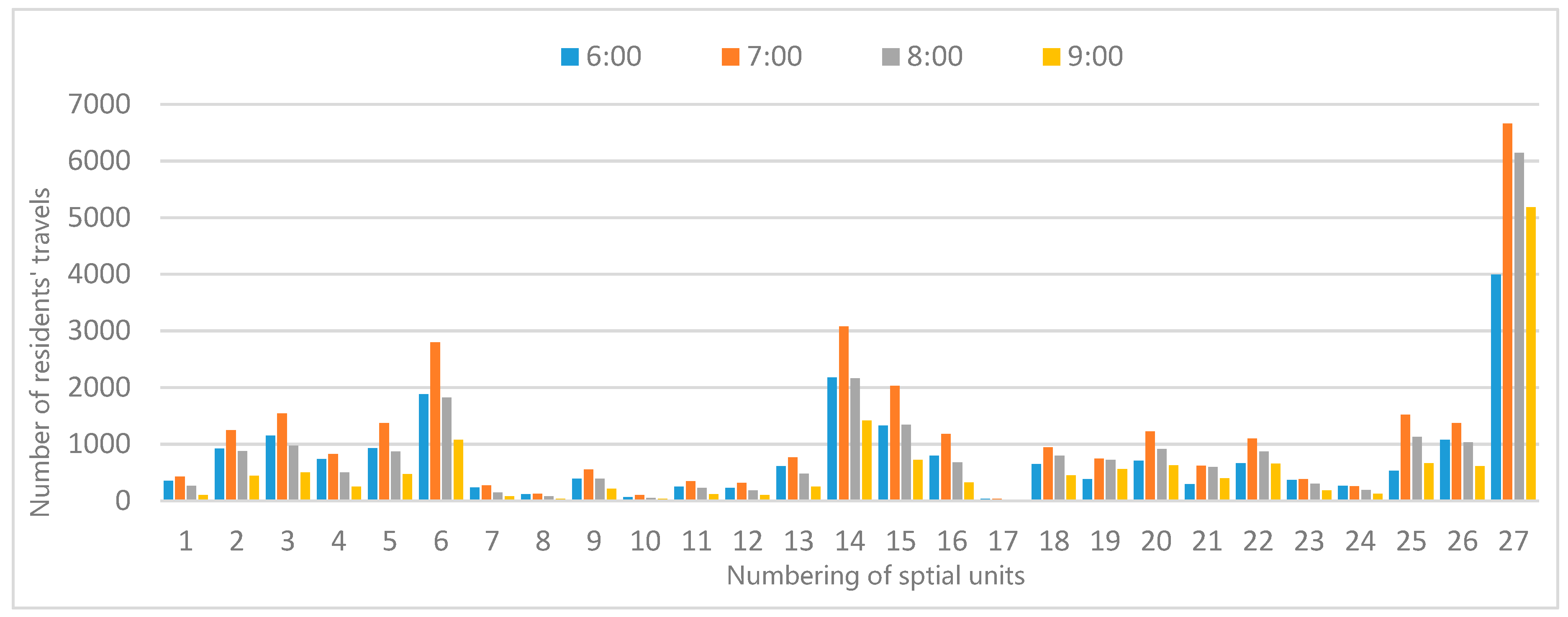
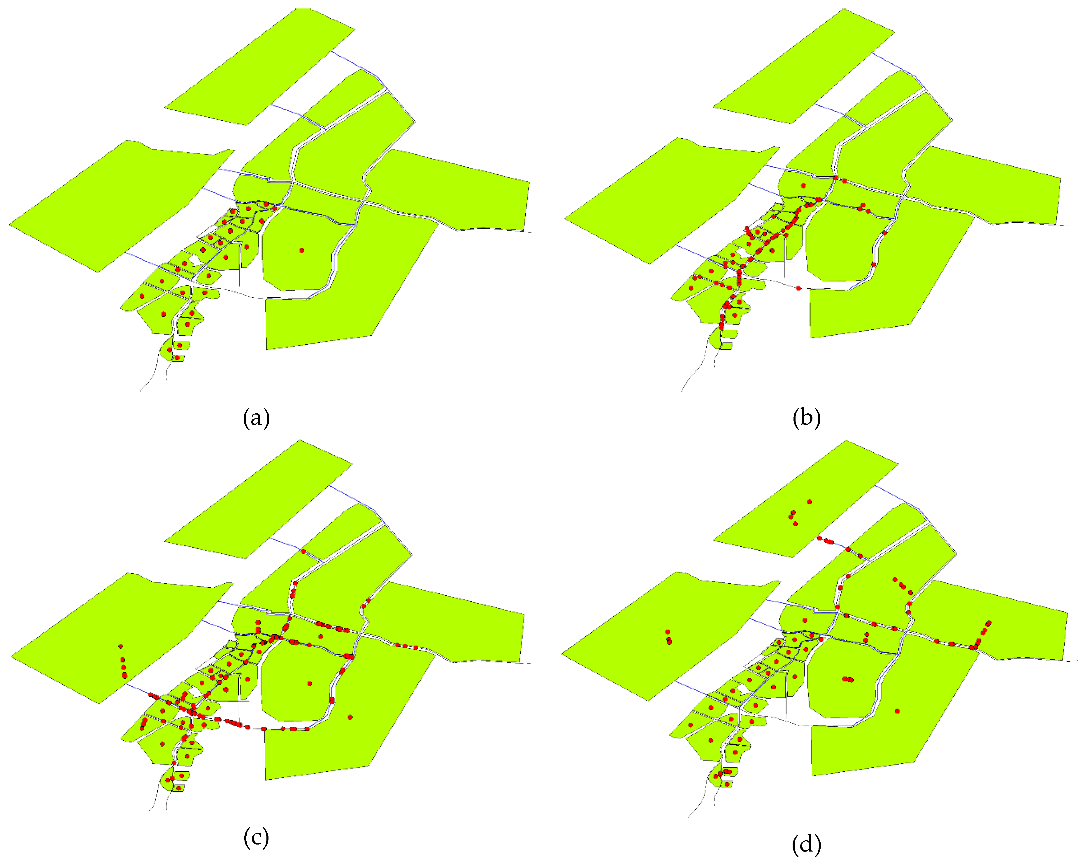
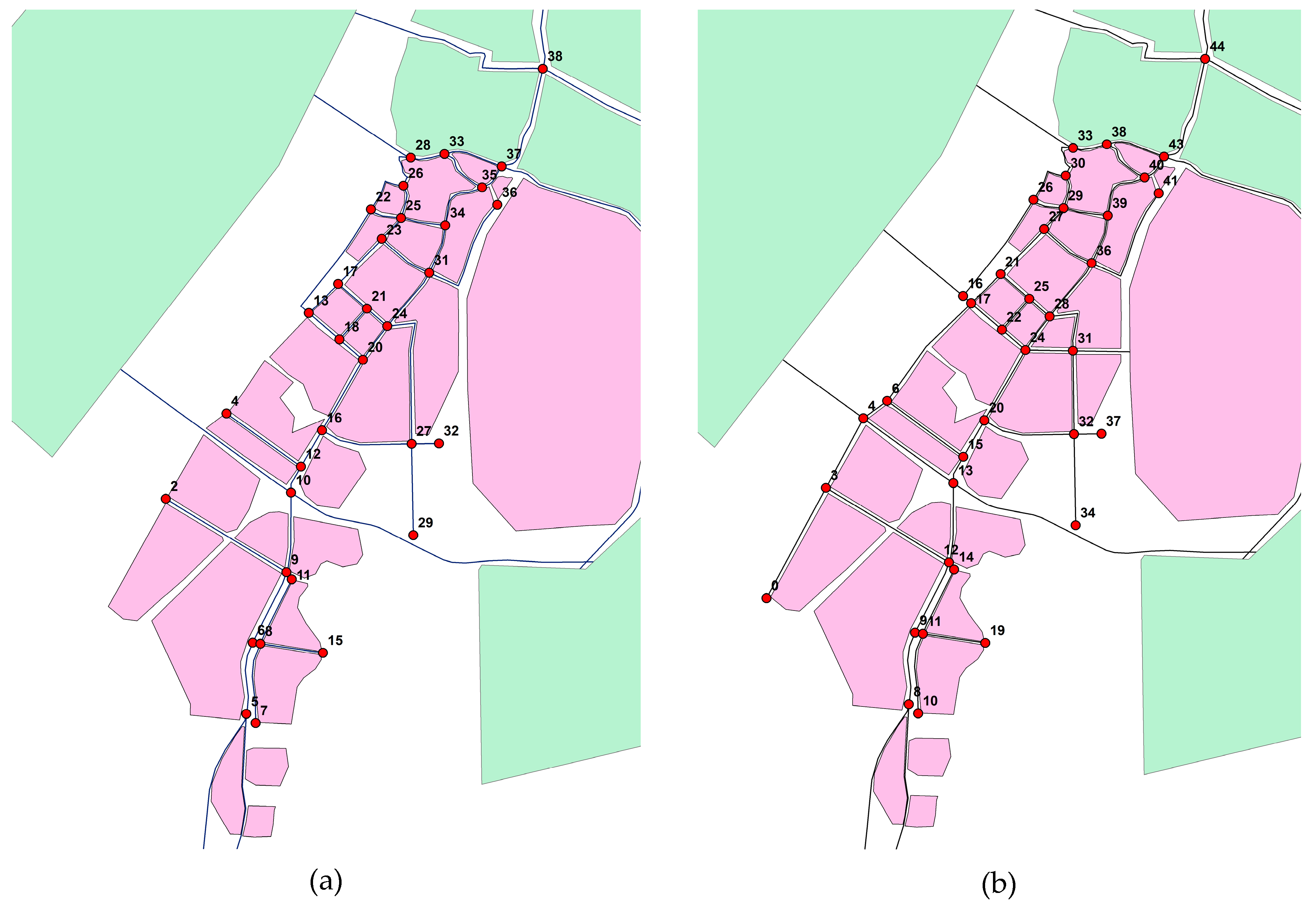
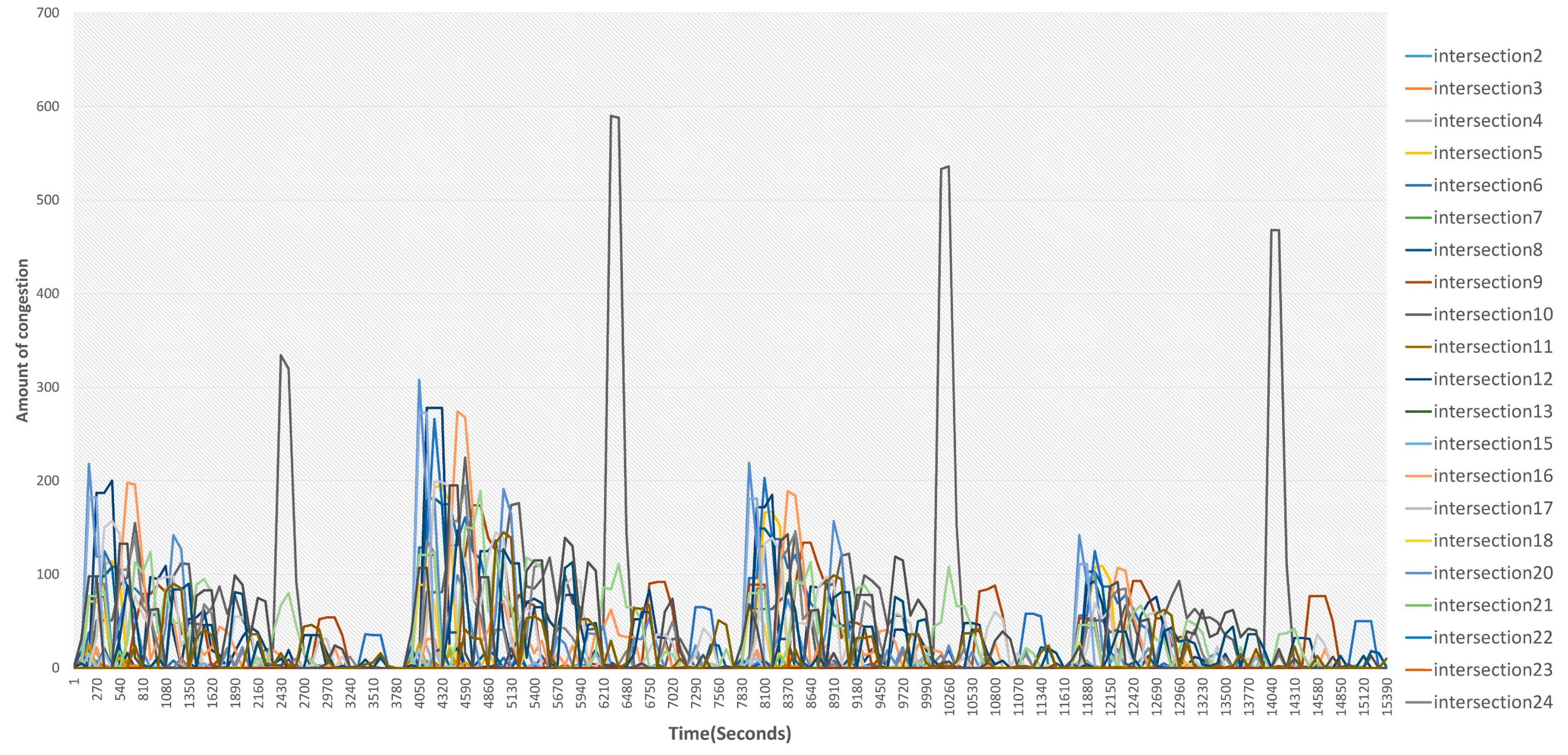
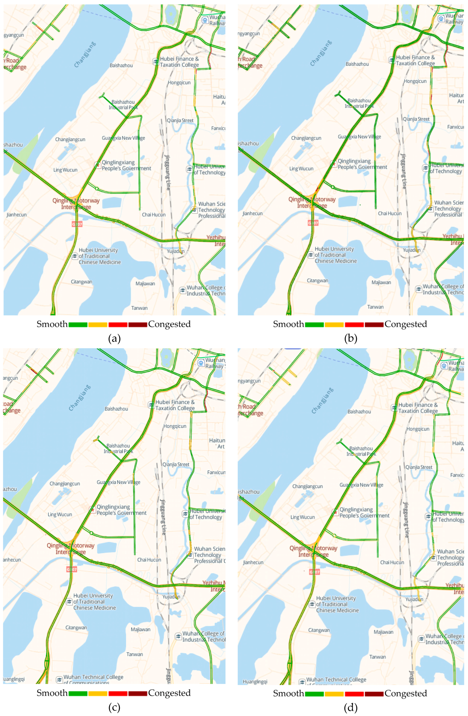
3.2. Model Simulation and Result Verification

Figure 5 presents real-time screenshot images at several time nodes during the running of the model. As the visual interface could not offer quantified traffic features, road intersections are numbered and the number of Agents at each running cycle is obtained in order to detect the occurrence, time, and level of traffic congestions. The numbering of road intersection is shown in Figure 6a.
Finally, the number of vehicles at each intersection in the study area was calculated in various periods each with a 90-s duration to obtain Figure 7. As shown by the changes in the number of agents at all intersections during various time periods, although differences can be seen in terms of the total number of commuter residents, the number of commuter residents on each plot, and the destinations of residents, the overall line charts generated for the four hours of study demonstrate a consistent pattern, representing similar features in the commuting of residents at each hour. Specifically, for road intersections, the peak in the line chart represents the maximum number of traffic generated, and the duration of time indicates the occurrence of congestion. Therefore, it can be seen that the most obvious congestion occurs at Intersection 10, i.e., the intersection of Baishazhou Avenue and the Third Ring Road. Other more congested intersections include No.6, No.9, and No.37.
Furthermore, the causes of congestion at each intersection can be analyzed. Combining the congestion process presentation at each intersection in the visual interface, and the number of residents departing from each block in different time periods (Table 3). Traffic in the surrounding area along the Baishazhou Avenue consists of two parts: commuting traffic from the area adjacent to Intersection 10 (the Qingling Interchange) to Plot 27 (the South Lake Area) and Plot 31 (the Optics Valley Area). While traffic in Intersection 37 (the Meijiashan interchange) comes from commuting to Plot 31 and Plot 30 (the Xudong Area). As a result, the commuting traffic flows have great impact on the road intersections near the two interchanges. In addition, as cross-river traffic in the entire area is still mainly directed to Plot 34, tension in traffic is mostly concentrated along the cross-river bridge (the Baishazhou Bridge) route.
Chinese web map providers, such as Gaode, Baidu, etc., provide not only navigation information, but also traffic forecasts based on their historical traffic data and projections of traffic conditions at different periods of a day. In the present study, traffic forecasts for the case study, the Baishazhou area, at the four time nodes, i.e., 7:00, 8:00, 9:00, and 10:00, are extracted from Gaode map as shown in Figure 8. Since these traffic forecasts are generated based on historical data, they can be considered as road traffic conditions with the highest probability of each road in the past years, and therefore, we used them in the study to verify the results of the model simulation.
Since Gaode’s data is only accurate to the hour and cannot be matched with the temporal granularity of traffic conditions in this simulation, comparisons can only be made on a similar time precision. Traffic at the end of each hour of simulation was used for the comparison, which means the simulation result for traffic starting at 6:00 was used for comparison with the traffic forecast at 7:00, and so on. It can be seen from the traffic forecast for Gaode that it covers only the city artery roads and above, but not the secondary roads or below, and the dark red, red, yellow, and green colors in the diagram represent increasingly better traffic conditions, from serious congestion to smooth flow. Therefore, it can be seen that the traffic condition is the worst at 8:00 when a dark red section appears at the Qingling Interchange at the intersection of Baishazhou Avenue and Third Ring Road, and the section is in yellow at the other three time nodes, indicating slight congestion. Another congestion occurs in sections along the Baishazhou Avenue ahead of and behind the Meijishan Interchange, where the heaviest traffic, in dark red color, also appears at the 8:00 time node while the sections are in yellow color at the other three time nodes. The rest of the time point is yellow. Compared to the roads in the model, intersections corresponding to the Qingling Interchange are Intersection 10, 12, and 16, while those corresponding to the Meijiahan Interchange are Intersection 35 and 37. It can be seen that most sections of congestion projected by Gaode are in accordance with the congested intersections as simulated in the model. Based on the above analysis, the results of the present model’s simulation are consistent with traffic forecasts of Gaode.

4. Discussion

Statistics in the OD matrix of residents’ travels at different hours show that, most of the spatial units follow the pattern of minimum traffic at 9:00, but there are also a few plots, such as Plot 27, that do not match the major pattern of travel numbers. Situated in the South Lake area and serving mainly residential functions, Plot 27 is one of the most congested areas in Wuhan during rush hours. A possible explanation is that the residents of the area choose to delay their departure time to 9:00 in order to avoid the traffic congestion period from 7:00 to 8:00, or they are stalled in traffic for too long and are considered as having not departed from the area in the statistics. This result, to some extent, verifies the significance of OD statistics and simulation by each hour: when the travel patterns of each space unit during the four hours change, traffic pressure at each intersection may also vary, and the causes behind these changes demand further analysis with the support of simulations. This is also why this study divides the unit time span of commuting travels into a one-hour basis.
In order to test the simulation results of the model for different schemes, and combined with the analysis of the causes of congestion, the roads in the study area are optimized according to the Wuhan master plan. As a measure of optimization, a waterfront north–south road along the Yangtze River and the road to the South Lake area are planned (Figure 6b). The planned and optimized road network is simulated in the model and compared with the original one. In this simulation, it is assumed that the population in this area remains unchanged and so do the places of residence and work. Comparing the simulation results of the two schemes (Figure 9), it can be seen that the optimized scheme is evidently better than the scheme before optimization: first, traffic has been distributed to multiple road intersections instead of being concentrated at an intersection before the optimization. Second, duration of traffic congestion is significantly shortened, which means congestions can be alleviated quickly even if they do occur.
According to Gaode’s Traffic Report on major cities in China, 81% of them suffer from congestions during rush hours of residents’ commuting [49]. Therefore, studying residents’ commuting behavior as a starting point to address the wider problem of urban traffic congestion bears practical significance, not only for China but also for the world at large. The era of big data is coming. When it is less difficult to acquire data, how to use them in urban research becomes an issue that calls for deliberation [40]. Previous studies prove that mobile phone call data can more accurately reflect the commuting features of urban residents. However, most studies focus on the overall analysis of cities on a macro scale and the visual representations. Few studies are found on the micro scale dynamic analysis of residents’ commuting behaviors, or on how commuting relates urban traffic.
However, as the sole data source used in the present study to understand residents’ mobility, CDR data still has limitations because it is a relatively sparse data in recording the travel trajectory of residents. It is difficult to obtain the traffic mode (or speed) of residents’ travel through statistical analysis. Thus, the specific correlations between commuter vehicles and mobile phone users are not discussed in the present study. Therefore, in follow-up studies, additional data sources such as bus card and traffic cameras at road intersections may facilitate the cross-examination of our research results or the setting rules of residents’ commuting at a finer time-scale. Of course, these rely on the availability of data, which remain difficult to collect compared with other sources at present.

5. Conclusions

In the present study, the Agent-based model is used to simulate traffic condition during commuting hours in a local urban area. First, the commuting demand of residents calculated by mobile phone data is used to simulate congestions on the existing urban road network. Then, data backtracking is used to identify the causes of congestion and to analyze the simulation results. Finally, the results of simulation are proven to be consistent with the actual traffic conditions. Although the data used are simplified for the easiness of processing and modeling, the study is still believed to be a positive endeavor of combining big data and ABM in an urban study, and it offers a valuable approach to studying residents’ commuting and urban traffic.
The approach used in the paper has several limitations that merit future consideration: first, vehicles other than commuter cars, such as buses are not considered. Prospective studies are expected to incorporate other available data sources and machine learning approaches to further specify modes of commuter travels and incorporate buses as a major means of transportation. Second, in the present model’s construction, lanes and traffic flow directions on the roads are not specified. In a congestion setting, only the density of vehicles in a certain section is considered while the overlapping of vehicles is neglected. This means that the model cannot sufficiently reflect traffic conditions in reality and also leads to the fact that the simulation results cannot be analyzed on a finer scale for deduction of the processes. Prospective studies are expected to further refine the road and traffic systems of the model.

Author Contributions

Conceptualization, Y.Y.; Methodology, L.L.; Validation, H.W. and L.L.; Formal Analysis, H.J.; Data Curation, Z.P.; Writing—Original Draft Preparation, H.W.; Writing—Review & Editing, Y.Y.; Project Administration, H.W.; Supervision, Z.P.; Funding Acquisition, H.W. and Q.N.

Funding

The research was funded by the China Postdoctoral Science Foundation (No. 2016M600609), the MOE Layout Foundation of Humanities and Social Sciences (No. 19YJCZH187); the National Natural Science Fund for Young Scholars (No. 51708425); the Natural Science Fund of China (No. 51778503); and the National Natural Science Fund for Young Scholars (No. 51708426).

Acknowledgments

The authors acknowledge the contribution of all the anonymous reviewers that improved the quality of the paper.

Conflicts of Interest

The authors declare no conflict of interest.

References

  1. Vickrey, W.S. Congestion Theory and Transport Investment. Am. Econ. Rev. 1969, 59, 251–260. [Google Scholar]
  2. Zhou, J.; Murphy, E.; Long, Y. Commuting efficiency in the Beijing metropolitan area: An exploration combining smartcard and travel survey data. J. Transp. Geogr. 2014, 41, 175–183. [Google Scholar] [CrossRef]
  3. Scott, D.M.; Kanaroglou, P.S.; Anderson, W.P. Impacts of commuting efficiency on congestion and emissions: Case of the Hamilton CMA, Canada. Transp. Res. Part D Transp. Environ. 1997, 2, 245–257. [Google Scholar] [CrossRef]
  4. Friedman, M.S.; Powell, K.E.; Hutwagner, L.; Graham, L.M.; Teague, W.G. Impact of changes in transportation and commuting behaviors during the 1996 Summer Olympic Games in Atlanta on air quality and childhood asthma. Jama J. Am. Med. Assoc. 2001, 285, 897–905. [Google Scholar] [CrossRef] [PubMed]
  5. Brueckner, J.K. Urban Sprawl: Diagnosis and Remedies. Int. Reg. Sci. Rev. 2000, 23, 160–171. [Google Scholar] [CrossRef]
  6. Arnott, R.; De Palma, A.; Lindsey, R. A structural model of peak-period congestion—A traffic bottleneck with elastic demand. Am. Econ. Rev. 1993, 83, 161–179. [Google Scholar]
  7. Anas, A.; Xu, R. Congestion, land use, and job dispersion: A general equilibrium model. J. Urban Econ. 1999, 45, 451–473. [Google Scholar] [CrossRef]
  8. Gonzales, E.J.; Daganzo, C.F. Morning commute with competing modes and distributed demand: User equilibrium, system optimum, and pricing. Transp. Res. Part B Methodol. 2012, 46, 1519–1534. [Google Scholar] [CrossRef] [Green Version]
  9. Chatman, D.G. Does TOD Need the T? On the Importance of Factors Other Than Rail Access. J. Am. Plan. Assoc. 2013, 79, 17–31. [Google Scholar] [CrossRef]
  10. Salon, D. Neighborhoods, cars, and commuting in New York City: A discrete choice approach. Transp. Res. Part A Policy Pract. 2009, 43, 180–196. [Google Scholar] [CrossRef] [Green Version]
  11. Fosgerau, M.; Kim, J.; Ranjan, A. Vickrey meets Alonso: Commute scheduling and congestion in a monocentric city. J. Urban Econ. 2018, 105, 40–53. [Google Scholar] [CrossRef]
  12. Song, C.M.; Koren, T.; Wang, P.; Barabasi, A.L. Modelling the scaling properties of human mobility. Nat. Phys. 2010, 6, 818–823. [Google Scholar] [CrossRef] [Green Version]
  13. Ratti, C.; Frenchman, D.; Pulselli, R.M.; Williams, S. Mobile Landscapes: Using Location Data from Cell Phones for Urban Analysis. Environ. Plan. B Plan. Des. 2006, 33, 727–748. [Google Scholar] [CrossRef]
  14. Wesolowski, A.; Eagle, N.; Tatem, A.J.; Smith, D.L.; Noor, A.M.; Snow, R.W.; Buckee, C.O. Quantifying the Impact of Human Mobility on Malaria. Science 2012, 338, 267–270. [Google Scholar] [CrossRef] [PubMed] [Green Version]
  15. Bengtsson, L.; Lu, X.; Thorson, A.; Garfield, R.; Von Schreeb, J. Improved Response to Disasters and Outbreaks by Tracking Population Movements with Mobile Phone Network Data: A Post-Earthquake Geospatial Study in Haiti. PLoS Med. 2011, 8, 8. [Google Scholar] [CrossRef] [PubMed]
  16. Calabrese, F.; Colonna, M.; Lovisolo, P.; Parata, D.; Ratti, C. Real-Time Urban Monitoring Using Cell Phones: A Case Study in Rome. Ieee Trans. Intell. Transp. Syst. 2011, 12, 141–151. [Google Scholar] [CrossRef]
  17. Aasa, A. Application of mobile phone location data in mapping of commuting patterns and functional regionalization: A pilot study of Estonia. J. Maps 2013, 9, 10–15. [Google Scholar]
  18. Kung, K.S.; Greco, K.; Sobolevsky, S.; Ratti, C. Exploring Universal Patterns in Human Home-Work Commuting from Mobile Phone Data. PLoS ONE 2014, 9, e96180. [Google Scholar] [CrossRef] [PubMed]
  19. Tu, W.; Cao, J.; Yue, Y.; Shaw, S.L.; Zhou, M.; Wang, Z.; Chang, X.; Xu, Y.; Li, Q. Coupling mobile phone and social media data: A new approach to understanding urban functions and diurnal patterns. Int. J. Geogr. Inf. Sci. 2017, 31, 2331–2358. [Google Scholar] [CrossRef]
  20. Yue, Y.; Zhuang, Y.; Yeh, A.G.; Xie, J.Y.; Ma, C.L.; Li, Q.Q. Measurements of POI-based mixed use and their relationships with neighbourhood vibrancy. Int. J. Geogr. Inf. Syst. 2017, 31, 658–675. [Google Scholar] [CrossRef]
  21. Doyle, J.; Hung, P.; Farrell, R.; McLoone, S. Population Mobility Dynamics Estimated from Mobile Telephony Data. J. Urban Technol. 2014, 21, 109–132. [Google Scholar] [CrossRef]
  22. Pei, T.; Sobolevsky, S.; Ratti, C.; Shaw, S.L.; Li, T.; Zhou, C. A new insight into land use classification based on aggregated mobile phone data. Int. J. Geogr. Inf. Sci. 2014, 28, 1988–2007. [Google Scholar] [CrossRef] [Green Version]
  23. Pei, T.; Sobolevsky, S.; Ratti, C.; Shaw, S.L.; Li, T.; Zhou, C. Development of origin-destination matrices using mobile phone call data. Transp. Res. Part C Emerg. Technol. 2014, 40, 63–74. [Google Scholar]
  24. Calabrese, G.F.; Lorenzo, D.; Liu, L.; Ratti, C. Estimating origin-destination flows using mobile phone location data. IEEE Pervasive Comput. 2011, 10, 264–323. [Google Scholar] [CrossRef]
  25. Alexander, L.; Jiang, S.; Murga, M.; González, M.C. Origin–destination trips by purpose and time of day inferred from mobile phone data. Transp. Res. Part C Emerg. Technol. 2015, 58, 240–250. [Google Scholar] [CrossRef]
  26. Yue, Y.; Lan, T.; Yeh, A.G.; Li, Q.Q. Zooming into individuals to understand the collective: A review of trajectory-based travel behaviour studies. Travel Behav. Soc. 2014, 1, 69–78. [Google Scholar] [CrossRef]
  27. Çolak, S.; Lima, A.; González, M.C. Understanding congested travel in urban areas. Nat. Commun. 2016, 7, 10793. [Google Scholar] [CrossRef]
  28. Yao, Y.; Hong, Y.; Wu, D.; Zhang, Y.; Guan, Q. Estimating the effects of "community opening" policy on alleviating traffic congestion in large Chinese cities by integrating ant colony optimization and complex network analyses. Comput. Environ. Urban Syst. 2018, 70, 163–174. [Google Scholar] [CrossRef]
  29. Nguyen, Q.T.; Bouju, A.; Estraillier, P. Multi-agent Architecture with Space-time Components for the Simulation of Urban Transportation Systems. Procedia Soc. Behav. Sci. 2012, 54, 365–374. [Google Scholar] [CrossRef] [Green Version]
  30. Doniec, A.; Mandiau, R.; Piechowiak, S.; Espié, S. A behavioral multi-agent model for road traffic simulation. Eng. Appl. Artif. Intell. 2008, 21, 1443–1454. [Google Scholar] [CrossRef]
  31. Ciari, F.; Balmer, M.; Axhausen, K.W. A new mode choice model for a multi-agent transport simulation. In Proceedings of the 8th Swiss Transport Research Conference, Ascona, Switzerland, 6–8 October 2008. [Google Scholar]
  32. Knapen, L.; Keren, D.; Cho, S.; Bellemans, T.; Janssens, D.; Wets, G. Analysis of the Co-routing Problem in Agent-based Carpooling Simulation. In Ant 2012 And Mobiwis 2012; Shakshuki, E., Younas, M., Eds.; Elsevier Science Bv: Amsterdam, The Netherlands, 2012; pp. 821–826. [Google Scholar]
  33. Kaddoura, I.; Kickhöfer, B.; Neumann, A.; Tirachini, A. Optimal Public Transport Pricing: Towards an Agent-based Marginal Social Cost Approach. J. Transp. Econ. Policy 2016, 49, 200–218. [Google Scholar]
  34. Dimitrov, S.; Ceder, A.; Chowdhury, S.; Monot, M. Modeling the interaction between buses, passengers and cars on a bus route using a multi-agent system. Transp. Plan. Technol. 2017, 40, 592–610. [Google Scholar] [CrossRef]
  35. Liu, J.; Kockelman, K.M.; Boesch, P.M.; Ciari, F. Tracking a system of shared autonomous vehicles across the Austin, Texas network using agent-based simulation. Transportation 2017, 44, 1261–1278. [Google Scholar] [CrossRef]
  36. Lu, M.; Hsu, S.C. Spatial Agent-based model for environmental assessment of passenger transportation. J. Urban Plan. Dev. 2017, 143, 04017016. [Google Scholar] [CrossRef]
  37. Bellemans, T.; Bothe, S.; Cho, S.; Giannotti, F.; Janssens, D.; Knapen, L.; Körner, C.; May, M.; Nanni, M.; Pedreschi, D.; et al. An Agent-Based Model to Evaluate Carpooling at Large Manufacturing Plants. In Ant 2012 And Mobiwis 2012; Shakshuki, E., Younas, M., Eds.; Elsevier Science Bv: Amsterdam, The Netherlands, 2012; pp. 1221–1227. [Google Scholar]
  38. Calabrese, F.; Ferrari, L.; Blondel, V.D. Urban Sensing Using Mobile Phone Network Data: A Survey of Research. Acm Comput. Surv. 2014, 47, 25. [Google Scholar] [CrossRef]
  39. Batty, M.; Axhausen, K.W.; Giannotti, F.; Pozdnoukhov, A.; Bazzani, A.; Wachowicz, M.; Ouzounis, G.; Portugali, Y. Smart cities of the future. Eur. Phys. J. Spec. Top. 2012, 214, 481–518. [Google Scholar] [CrossRef] [Green Version]
  40. Wu, H.; Liu, L.; Yu, Y.; Peng, Z. Evaluation and Planning of Urban Green Space Distribution Based on Mobile Phone Data and Two-Step Floating Catchment Area Method. Sustainability 2018, 10, 214. [Google Scholar] [CrossRef]
  41. Song, C.; Qu, Z.; Blumm, N.; Barabási, A.L. Limits of Predictability in Human Mobility. Science 2010, 327, 1018–1021. [Google Scholar] [CrossRef] [Green Version]
  42. Yang, C.; Zhang, Y.; Ukkusuri, S.V.; Zhu, R. Mobility Pattern Identification Based on Mobile Phone Data. In Transportation Analytics in the Era of Big Data; Ukkusuri, S.V., Yang, C., Eds.; Springer International Publishing: Basel, Switzerland, 2012; pp. 217–232. [Google Scholar]
  43. Levy, S.; Martens, K.; Van Der Heijden, R. Agent-based models and self-organisation: : Addressing common criticisms and the role of agent-based modelling in urban planning. Town Plan. Rev. 2016, 87, 321–338. [Google Scholar] [CrossRef]
  44. Malleson, N. Extending RepastCity. 2012. Available online: https://code.google.com/p/repastcity/wiki/ExtendingRepastCity3 (accessed on 23 July 2019).
  45. Malleson, N. RepastCity-Model Structure. 2012. Available online: https://code.google.com/p/repastcity/wiki/RC3ModelStructure (accessed on 23 July 2019).
  46. Malleson, N. RepastCity-A Demo Virtual City. 2012. Available online: https://code.google.com/p/repastcity/wiki/RepastCity3 (accessed on 23 July 2019).
  47. Kopf, J.; Ishimaru, J.M.; Nee, J.; Hallenbeck, M.E. Central Puget Sound Freeway Network Usage and Performance, 2003 Update. Highway Traffic Control. 2005. Available online: http://www.highwaytraffic.com.au/#!/ (accessed on 23 July 2019).
  48. Widyantoro, D.H.; Munajat, M.E. Fuzzy traffic congestion model based on speed and density of vehicle. In Proceedings of the 2014 International Conference of Advanced Informatics: Concept, Theory and Application, Bandung, Indonesia, 20–21 August 2014. [Google Scholar]
  49. Gaode Map. Traffic Report on Major Cities in China 2017. 2018. Available online: http://cn-hangzhou.oss-pub.aliyun-inc.com/download-report/download/yearly_report/2017/ (accessed on 23 July 2019).
Figure 1. Procedures of assigning a user to a spatial unit.
Ijgi 08 00313 g001
Figure 2. Diagram of rules for resident Agent behavior.
Ijgi 08 00313 g002
Figure 3. Road network and division of urban spatial units. (a) The original blocks and road network; (b) Simplified spatial units of land use and road network; (c) Names of key Roads and spatial units.
Ijgi 08 00313 g003
Figure 4. Comparison of residents’ travels at different hours in different spatial units.
Ijgi 08 00313 g004
Figure 5. Real-time screenshots during model running and simulation. (a) Run time 30 s; (b) Run time 900 s; (c) Run time 1800 s; (d) Run time 3200 s.
Ijgi 08 00313 g005
Figure 6. Numbering and distribution of road intersections. (a) Numbering and distribution of existing road intersections; (b) Numbering and distribution of planned road intersections.
Ijgi 08 00313 g006
Figure 7. Changes in the number of agents at intersections.
Ijgi 08 00313 g007
Figure 8. Traffic forecasts for the four studied hours based on the big data from Gaode Map. (a) 7:00 traffic conditions; (b) 8:00 traffic conditions; (c) 9:00 traffic conditions; (d) 10:00 traffic conditions.
Ijgi 08 00313 g008
Figure 9. Comparison of traffic conditions before and after the optimization of the road network. (a) The traffic conditions of road intersections before optimization; (b) The traffic conditions of road intersections after optimization.
Ijgi 08 00313 g009
Table 1. Sample of mobile phone call data.
User IDTime of Phone CallBase Station ID
100000012016-03-09-9.11.49.000000287305843
100000022016-03-09-9.15.24.0000005760859194
100000032016-03-09-9.15.18.0000002872636812
100000042016-03-09-9.15.49.0000002893525929
100000052016-03-09-9.24.13.0000002871037354
Table 2. Sample statistics of base stations assigned to user ID at different hours of a day.
User IDBase Station ID at 7:00Base Station ID at 8:00Base Station ID at 9:00Base Station ID at 10:00Base Station ID at 11:00
1000000128978256432870117513287011751328701403382897825643
1000000228718654152871865415287186541528718654152871865415
1000000328701246052870125269289346302528934100622893463025
1000000428962122612870140337287012951128701295112870129511
1000000528971121722897112173289711217228971554040
1000000628968576362896840168289682935628730445332896851574
1000000729195499322919543433291954993229195499322919440084
Table 3. Sample statistics of travel volume at each hour and at each plot.
Departure Lot No.Destination Lot No.Departure at 6:00Departure at 7:00Departure at 8:00Departure at 9:00
132010100
142020200
1910000
11401000

