Dynamic Deployment of Wireless Sensor Networks by Biogeography Based Optimization Algorithm

Abstract

As the usage and development of wireless sensor networks increases, problems related to these networks are becoming apparent. Dynamic deployment is one of the main topics that directly affects the performance of the wireless sensor networks. In this paper, biogeography-based optimization is applied to the dynamic deployment of static and mobile sensor networks to achieve better performance by trying to increase the coverage area of the network. A binary detection model is considered to obtain realistic results while computing the effectively covered area. Performance of the algorithm is compared with that of the artificial bee colony algorithm, Homo-H-VFCPSO and stud genetic algorithm that are also population-based optimization algorithms. Results show biogeography-based optimization can be preferable in the dynamic deployment of wireless sensor networks.

1. Introduction

Wireless sensor networks (WSNs) are used for vehicle tracking, environment monitoring, healthcare and for getting temperature, pressure data, light, humidity, etc. and obtaining information about things such as the weight, movement direction, and velocity of an object in an area of interest [1]. Regardless of which network is used in many applications, the success of the network is highly dependent on the sensors’ positions, referred to as the deployment of the network. Deciding the positions of the sensors is the main subject of sensor network deployment, and in turn it depends on the desired coverage of the area of interest. With regard to the dynamic deployment problem, initially sensors are located in the area in random positions and the sensors change their positions by using the knowledge of others positions, if they are mobile. These movements attempt to increase the coverage rate of the sensors. However, if the sensors are static, they do not have the ability to change their positions.

In initial deployment, because of the randomness of the method, generally an effective coverage cannot be obtained. To tackle this problem, various dynamic deployment algorithms have been studied by researchers [2,3,4,5]. To improve the coverage of the network, one of the approaches used in these researches is the Artificial Bee Colony (ABC) algorithm [6], which works well for WSNs which consist only of mobile sensors [6,7,8]. Abderrahim et al. used an approach for the deployment of WSN based on the use of Simulated Annealing (SA) to obtain close to optimal solutions for the placement of sensors in terms of minimizing the number of hops between all the nodes of the target region and the sink node while covering as much of the area of interest as possible. By reducing the number of hops, energy saving is also improved [9]. In [10], an optimization model for traffic monitoring based on the Artificial Fish School Algorithm (AFSA) was proposed for dynamic deployment of mobile sensor networks. These approaches are not relevant for static sensors which are unable to change their initial positions. However, static sensors are widely used in real life network applications in order to reduce costs and save energy. Wang et al. considered both static and mobile sensors together in WSNs and proposed some new approaches: one based on parallel particle swarm optimization (PPSO) [11]; VFCPSO algorithm based on VF algorithm; and co-evolutionary particle swarm optimization (CPSO) [12]. Recently, for the purpose of investigating the performance of different paradigms, Wang et al. extended centralized VFCPSO to distributed VFCPSO, heterogeneous hierarchical VFCPSO and homogeneous hierarchical VFCPSO (Homo-H-VFCPSO), and analyzed solutions for preferential deployment in the region of interest. Simulation results demonstrate that the Homo-H-VFCPSO performed better than the three other VFCPSO algorithms and the VF-style algorithms in terms of computation time, coverage and efficient energy consumption [13]. In [14], Rani et al. proposed a multi-objective PSO and fuzzy based optimization model for sensor node deployment in which the main objective considered is to maximize network coverage, connectivity and network lifetime, thus maximizing the coverage and detection probabilities. Ahmed et al. addressed the problem of determining the current coverage achieved by the non-deterministic deployment of static sensor nodes and subsequently enhancing the coverage using mobile sensors [15]. They identify three key elements that are critical for ensuring effective area coverage in Hybrid WSN: (i) determining the boundary of the target region and evaluating the area coverage; (ii) locating coverage holes and maneuvering mobile nodes to fill these voids; and (iii) maintaining the desired coverage over the entire operational lifetime of the network. They then proposed a comprehensive solution that addresses all of the aforementioned aspects of the area coverage, called mobility assisted probabilistic coverage (MAPC) which is a distributed protocol that operates in three distinct phases. The first phase identifies the boundary nodes using the geometric right-hand rule. Next, the static nodes calculate the area coverage and identify coverage holes using a novel probabilistic coverage algorithm (PCA) which incorporates a realistic sensing coverage model for range-based sensors. The second phase of MAPC is responsible for navigating the mobile nodes to plug the coverage holes. They proposed a set of coverage and energy-aware variants of the basic virtual force algorithm (VFA). Finally, the third phase addresses the problem of coverage loss due to faulty and energy depleted nodes. They formulate a deployment problem as an Integer Linear Program (ILP) and propose practical heuristic solutions that achieve similar performance to that of the optimal ILP solution.

In this study, a new approach for dynamic deployment problem for WSNs is proposed. We considered WSNs which combine mobile and static sensors. This approach is based on the Biogeography-Based Optimization (BBO) algorithm which is inspired by the immigration and emigration of species between islands (or habitats) in search of more compatible islands [16]. It is known that the BBO algorithm and its variants work well for many optimization problems [17,18,19]. As far as we know, the BBO algorithm was initially used on dynamic deployment for WSN. Considering the good performance of the algorithm, use of the BBO algorithm seemed an appropriate approach to enable the sensors in the network to obtain a good coverage in two dimensional space with static and mobile nodes. The performance of the proposed approach is evaluated in comparison with other population-based algorithms, such as the Artificial Bee Colony (ABC) algorithm, Homo-H-VFCPSO and Stud Genetic Algorithm (SGA).

The rest of this paper is structured as follows: Section 2 describes the mathematical model in dynamic deployment problem for WSN. Subsequently, the proposed approach is presented in Section 3 and the detailed implementation procedure is also described. The simulation experiment is implemented and comparison of ABC, Homo-H-VFCPSO, SGA and the proposed approach for this problem is described in Section 4. Section 5 consists of the conclusion and proposals for future work.

2. WSN Dynamic Deployment Problem and Sensor Detection Model

The performance of a sensor network depends on its position in the area of interest. Therefore, by responding to all system objectives, deployment of the sensors in the mission space is a problem which is called the sensing coverage, coverage control or active sensing problem [20,21,22,23]. In the applications which consider coverage, sensors should be deployed to maximize the information that they collect from the area of interest. In the case of static networks, after the sensors’ first positioning, no further mobility is possible and optimal locations are found by using an off-line scheme as a facility location optimizer. Whereas, in the dynamic version of the networks, sensors are able to move coordinately within the mission space [24].

In WSNs, sensors can collect information about the area within their detection ranges. They share their information with neighboring sensors as well as with base stations. Therefore, for effective detection in a network, including communications from sensors the covered area should be expanded. In order to increase the ratio of the covered area, mobile sensors’ positions maneuverability can be utilized.

Since there is no priori information about the sensing area, initial positions of the sensors are chosen randomly and deployment of sensors in the area of interest will be obtained dynamically. The sensor field is a two-dimensional grid. Each sensor knows its position. Sensors communicate with each other and the mobile ones can change their positions by using this information. Coverage ratio of the WSN is calculated by Equation (1) [29]:

where c_i is the coverage of a sensor i, S is the set of the nodes, and A is the total size of the area of interest. The reason why a union operation is used rather than a plus operation, is that every grid point is calculated only once.

There are two sensor detection models in WSNs to find effective coverage. One of them is a binary detection model which assumes that there is no uncertainty and the other is the stochastic detection model. In this paper, we used the binary detection model which assumes that there is no uncertainty. Assuming that, there are k sensors in the random deployment stage, each sensor has the same detection range r, sensor s_i is positioned at (x_i, y_i). For any point P at (x, y), Euclidean distance between s_i and P is d(s_i, P). The binary sensor model [25] is shown by Equation (2):

where c_xy(s_i) is the coverage of a grid point P by sensor s_i, d(s_i, P) is Euclidean distance. For simplicity, but without loss of generality, we use the binary sensor model to confirm the effectiveness of BBO in solving the sensor deployment.

3. Dynamic Deployment of Wireless Sensor Networks with Biogeography-Based Optimization

Biogeography-Based Optimization (BBO) [16] was proposed by Simon in IEEE Transactions on Evolutionary Computation in 2008. BBO is a new evolution algorithm developed for the global optimization. It is inspired by the immigration and emigration of species between islands (or habitats) in search of more compatible islands. In our work, the Biogeography-Based Optimization algorithm is used for the dynamic deployment problem of WSNs. The reason for using the optimization algorithm is to maximize the coverage rate of the network, given with Equation (1) where it is assumed within the network scenario:

• Detection radii of the sensors are all identical (r);
• All of the sensors have ability to communicate with other sensors;
• WSN consists of both mobile and static sensors.

In the BBO algorithm, each candidate solution is called a “habitat” (or “island”) with a Habitat Suitability Index (HSI) and denoted by an n-dimension real vector. Therefore, the deployment of the sensors in the area covered refers to a habitat (a solution) in the algorithm. The coverage rate of the network, i.e., total covered area, corresponds to the fitness value (HSI) of the solution. In the BBO model, an initial entity in the habitat vector is generated at random. The habitat with a high HSI is considered to be optimal, while the habitat with a low HSI is unfavorable. Low HSI, however, may incorporate some positive traits from the high HSI that could well become high HSI solutions. 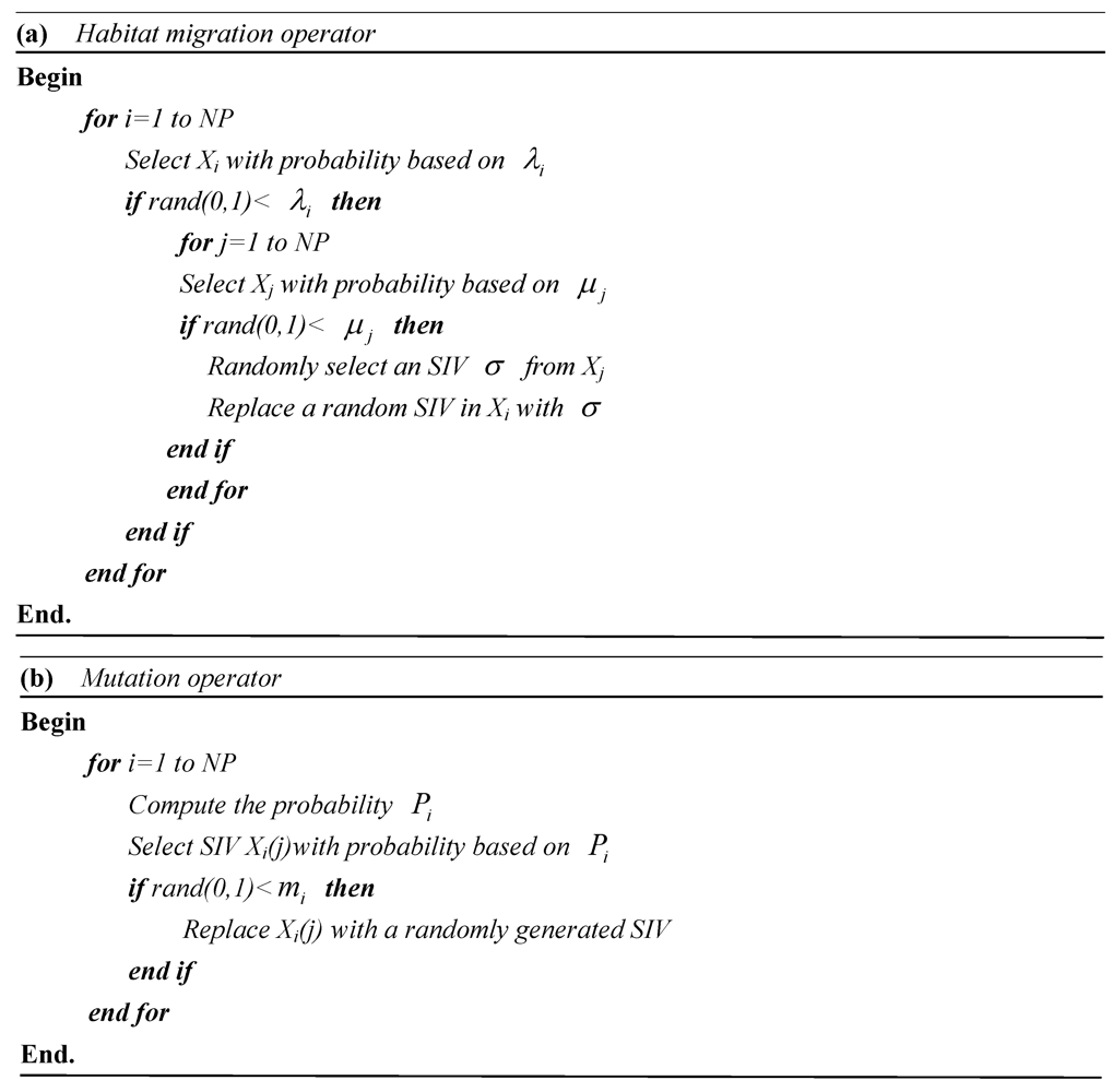In BBO, habitat H (generally speaking, we use X in real application problem) is a vector of n Suitable Index Vectors (SIVs) generated randomly, then migration and mutation operations are implemented to achieve an optimal solution. The new candidate solution is generated from the entire habitat in population by using the migration and mutation operator shown in Figure 1.

In BBO, the migration strategy is similar to the evolutionary strategy (ES) in which a single offspring can be produced by many parents. BBO migration operator can change existing habitats and modify existing solutions. Migration is a probabilistic operator that adjusts habitat X_i. The modified probability X_i is proportional to its immigration rate λ_i, and the source of the modified probability from X_j is proportional to the emigration rate μ_j. The migration operator is shown in Figure 1(a).

Figure 1. (a) The habitat migration operator algorithm. (b) The habitat mutation operator algorithm.

Figure 1. (a) The habitat migration operator algorithm. (b) The habitat mutation operator algorithm.

Mutation is also a probabilistic operator that randomly modifies habitat SIVs based on the habitat priori probability of existence. Very high HSI solutions and very low HSI solutions are equally improbable. Medium HSI solutions are relatively probable.

Additionally, the mutation operator tends to increase the population diversity. Mutation can be described as shown in Figure 1(b). The basic framework of BBO algorithm can be simply described as as shown in [16]. More details about the migration operator, mutation operator and BBO algorithm can be found in [16] and in the MATLAB code [26].

The steps of the BBO algorithm for the dynamic deployment problem of WSNs are:

• - Initialize the parameters: detection radius r, size of the area of interest A, number of mobile sensors m, number of static sensors s, population size NP, maximum number of iterations MaxGeneration, divided grid size GridSize, maximum variation rate m_max, migration rate p_mod, the maximum capacity of habitat species S_max, maximum of immigration operator I and maximum of emigration operator E and the maximum of elite individuals retained z.
• - Deploy the s static sensors at random.
• - Determine the positions of m mobile sensors randomly for each Habitat X_i using Equation (3) where j = 1, 2,…, 2m:
• - Evaluate the fitness value (HSI, i.e., coverage rate) for each individual.
• - t = 0
• - REPEAT
  • - Sort the population from worst to best according to its HSI.
  • - For each individual, map the HSI to the number of species using Equation (4), where m_max is a user-defined parameter, P_s and P_max is migration rate for S species and max species respectively:
  • - Calculate the immigration rate λ_i and the emigration rate μ_i for each individual x_i.
  • - Modify the population with the migration operator shown in Figure 1(a).
  • - Update the probability of each individual.
  • - Mutate the population with the mutation operator shown in Figure 1(b).
  • - Evaluate the fitness for each individual.
  • - Memorize the best solution achieved so far.
  • - t = t + 1
• - UNTIL t = MaxNumber

In the algorithm, as with other population-based optimization algorithms, we typically incorporate some sort of elitism in order to retain the best solutions in the population. This prevents the best solutions from being corrupted by immigration. z is the elitism parameter which signifies how many of the best habitats to keep from one generation to the next. Species are made of all the habitats, i.e., X₁, X₂,…, X_NP. x_i is the initial position of Sensor s_i determined by Equation (3), where x_i=(x_i,1, x_i,2,⋯, x_i,j, ⋯, x_i,2m-1, x_i,2m), 1 ≤ j ≤ 2m. In our work, min_j and max_j are 0 and 100, respectively. S_max is the largest possible number of species that the habitat can support. The immigration rate and the emigration rate are functions of the number of species in the habitat and are represented by migration rate p_mod for simplicity, whose maximum is a user-defined parameter m_max in Equation (4).

Each solution represents an array which has 2m items. Table 1 shows a solution array. Items of the solution array are (x, y) positions of the mobile sensors in the network.

Table 1. Solution array.

1	2	3	4	5	6	⋯	2m − 1	2m
x1	y1	x2	y2	x3	y3	⋯	xm	ym

Table 1. Solution array.

1	2	3	4	5	6	⋯	2m − 1	2m
x1	y1	x2	y2	x3	y3	⋯	xm	ym

4. Simulation Results

In this work, the performance of the BBO algorithm on dynamic deployment of WSNs is compared with the results of other algorithms: Artificial Bee Colony (ABC) [27], Homo-H-VFCPSO [13] and Stud Genetic Algorithm (SGA) [28]. The Artificial Bee Colony (ABC) algorithm is a swarm based intelligent optimization algorithm inspired by modeling the foraging behavior of bees. Homo-H-VFCPSO is a homogeneous hierarchical VFCPSOA algorithm initially proposed in 2011. The Stud Genetic Algorithm (SGA) is an improved Genetic Algorithm (GA) that uses the best individual at each generation for crossover.

In the simulations, a wireless sensor network including 20 mobile and 80 static sensors is simulated as described in [29]. Detection radius of the each sensor r is 7 m, the range detection error r_e is 0.5 × r = 3.5 m, size of the area which is a square region A (100 m × 100 m) is 10,000 m².

The BBO algorithms’ control parameters are set as follows (i.e., the same as in [16]): the population size NP is 30, habitat modification probability is 1, immigration probability bounds per gene is [0,1], maximum immigration m_max and migration rates p_mod for each island is 1 and mutation probability is 0.005. The ABC algorithms’ population size NP is 30, limit parameter for the scout is taken as 100. SGA algorithms’ population size NP is 30, crossover probability is taken 1, and initial mutation probability is 0.01. The Homo-H-VFCPSO algorithms’ control parameters are set as in [13]. We did some fine tuning on each of the optimization algorithms except BBO to obtain optimal performance, but we did not make any special efforts to tune the algorithm BBO, because Simon [16] has demonstrated that BBO is insensitive to the control parameter.

To allow a fair comparison of running times, all the experiments were performed on a PC with an AMD Athlon(tm) 64 X2 Dual Core Processor 4200+ running at 2.20 GHz, 1,024 MB of RAM and a hard drive of 160 Gbytes. Our implementation was compiled using MATLAB R2012a (7.14) running under Windows XP SP3. No commercial BBO tools or other population-based optimization tools were used in the experiments.

To compare the performance among the algorithms ABC, Homo-H-VFCPSO, BBO and SGA, we ran 100 Monte Carlo simulations of each algorithm on the binary dynamic deployment of WSNs to get representative performances with random initialization. The results are recorded in Table 2 after 100 Monte Carlo runs. In the table, standard deviation of 100 runs, consuming CPU time, the best and the worst of the runs are reported. We must point out that MG is short for the variable MaxGeneration in Table 2.

As seen from Table 2, the BBO algorithm is more successful than the ABC, Homo-H-VFCPSO and SGA for the dynamic deployment problem of WSNs using a binary detection model. In addition, the simulation results show that the deployments found by BBO are better than the deployments found by ABC, Homo-H-VFCPSO and SGA for most of the 100 independent runs started with random deployment.

Table 2. Binary Dynamic Deployment Results on Different Iterations.

		Initial coverage of stationery sensors	ABC	BBO	SGA	Homo-H-VFCPSO
MG = 50	Mean	0.6823	0.8367	0.8641	0.8262	0.8013
	Std	0.0254	0.0155	0.0134	0.0195	0.0158
	Best	0.7275	0.8728	0.9007	0.864	0.882
	Worst	0.6224	0.8049	0.8299	0.7699	0.8129
	Time(s)	-	31.7	15.61	15.35	17.03
MG =100	Mean	0.6762	0.854	0.8711	0.8375	0.8609
	Std	0.0248	0.0853	0.0868	0.0839	0.0889
	Best	0.7434	0.8896	0.9097	0.8769	0.8976
	Worst	0.6138	0.8115	0.8299	0.7962	0.7692
	Time(s)	-	80.55	36.97	35.36	36.53
MG = 500	Mean	0.683	0.8889	0.9184	0.8602	0.8536
	Std	0.0262	0.0885	0.0118	0.0856	0.0865
	Best	0.7346	0.9218	0.9519	0.8922	0.8299
	Worst	0.6131	0.8501	0.8798	0.8277	0.8188
	Time(sec)	-	356.77	173.28	175.07	185.15
MG = 1000	Mean	0.3783	0.8959	0.929	0.8709	0.8906
	Std	0.0241	0.0891	0.0122	0.0871	0.079
	Best	0.7495	0.9327	0.9523	0.9112	0.8989
	Worst	0.6224	0.8636	0.8956	0.8287	0.8829
	Time(s)	-	724.96	346.91	349.73	356.36

Table 2. Binary Dynamic Deployment Results on Different Iterations.

		Initial coverage of stationery sensors	ABC	BBO	SGA	Homo-H-VFCPSO
MG = 50	Mean	0.6823	0.8367	0.8641	0.8262	0.8013
	Std	0.0254	0.0155	0.0134	0.0195	0.0158
	Best	0.7275	0.8728	0.9007	0.864	0.882
	Worst	0.6224	0.8049	0.8299	0.7699	0.8129
	Time(s)	-	31.7	15.61	15.35	17.03
MG =100	Mean	0.6762	0.854	0.8711	0.8375	0.8609
	Std	0.0248	0.0853	0.0868	0.0839	0.0889
	Best	0.7434	0.8896	0.9097	0.8769	0.8976
	Worst	0.6138	0.8115	0.8299	0.7962	0.7692
	Time(s)	-	80.55	36.97	35.36	36.53
MG = 500	Mean	0.683	0.8889	0.9184	0.8602	0.8536
	Std	0.0262	0.0885	0.0118	0.0856	0.0865
	Best	0.7346	0.9218	0.9519	0.8922	0.8299
	Worst	0.6131	0.8501	0.8798	0.8277	0.8188
	Time(sec)	-	356.77	173.28	175.07	185.15
MG = 1000	Mean	0.3783	0.8959	0.929	0.8709	0.8906
	Std	0.0241	0.0891	0.0122	0.0871	0.079
	Best	0.7495	0.9327	0.9523	0.9112	0.8989
	Worst	0.6224	0.8636	0.8956	0.8287	0.8829
	Time(s)	-	724.96	346.91	349.73	356.36

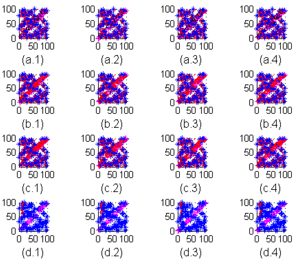
Figure 2. Best solutions of ABC: (a.1) iteration #50, (a.2) iteration #100, (a.3) iteration #500, (a.4) iteration #1000. Best solutions of BBO: (b.1) iteration #50, (b.2) iteration #100, (b.3) iteration #500, (b.4) iteration #1000. Best solutions of SGA: (c.1) iteration #50, (c.2) iteration #100, (c.3) iteration #500, (c.4) iteration #1000. Best solutions of Homo-H-VFCPSO: (c.1) iteration #50, (c.2) iteration #100, (c.3) iteration #500, (c.4) iteration #1000.

Figure 2. Best solutions of ABC: (a.1) iteration #50, (a.2) iteration #100, (a.3) iteration #500, (a.4) iteration #1000. Best solutions of BBO: (b.1) iteration #50, (b.2) iteration #100, (b.3) iteration #500, (b.4) iteration #1000. Best solutions of SGA: (c.1) iteration #50, (c.2) iteration #100, (c.3) iteration #500, (c.4) iteration #1000. Best solutions of Homo-H-VFCPSO: (c.1) iteration #50, (c.2) iteration #100, (c.3) iteration #500, (c.4) iteration #1000.

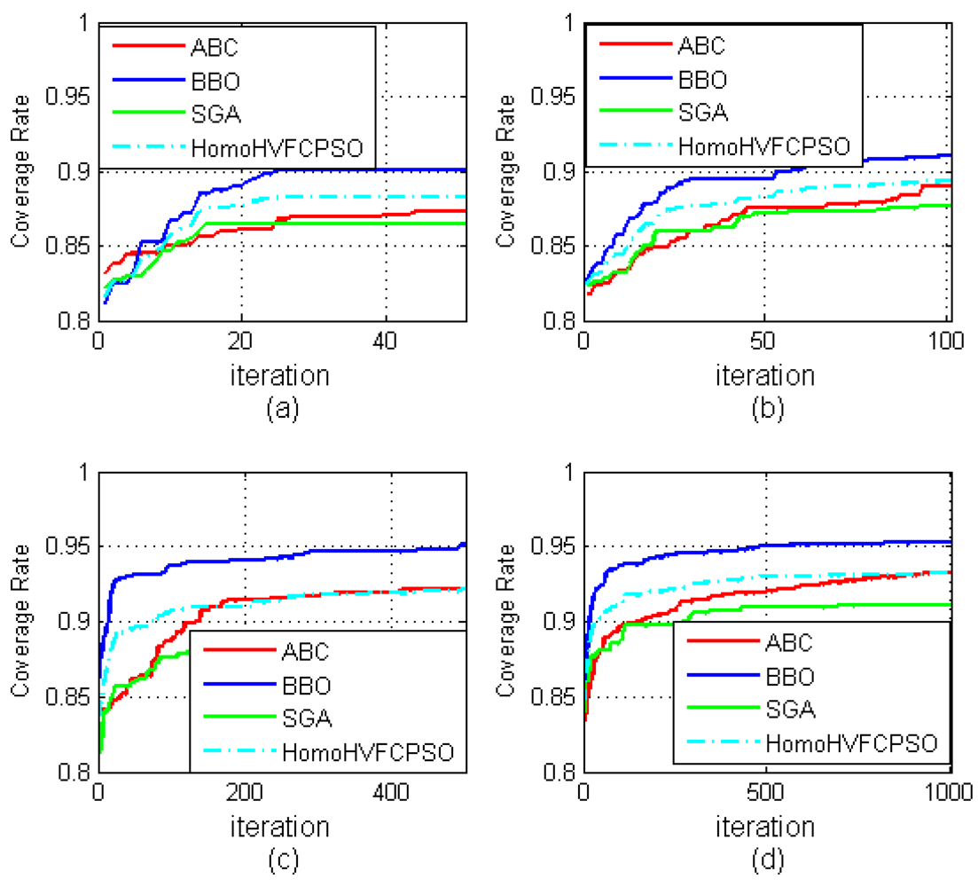
To observe the development of the best solutions for the algorithms through the iterations, refer to Figure 2 and Figure 3. In Figure 2, the convergences of four algorithms are shown by coverage rate for the iterations: iteration number 50, iteration number 100, iteration number 500, and iteration number 1,000 respectively. Figure 3, including development graphics of the average of the populations through the different iterations for ABC, BBO, Homo-H-VFCPSO and SGA, demonstrates that the BBO algorithm finds better deployments, and faster, than the other algorithms. Figure 3 demonstrates the convergence graphic of mean of average solutions of 100 Monte Carlo simulations for the different iterations: iteration number 50, iteration number 100, iteration number 500, and iteration number 1,000.

Figure 3. Average development of the populations through the different iterations for ABC, BBO, Homo-H-VFCPSO and SGA algorithms in 100 Monte Carlo simulations: (a) iteration #50, (b) iteration #100, (c) iteration #500, (d) iteration #1000.

Figure 3. Average development of the populations through the different iterations for ABC, BBO, Homo-H-VFCPSO and SGA algorithms in 100 Monte Carlo simulations: (a) iteration #50, (b) iteration #100, (c) iteration #500, (d) iteration #1000.

5. Conclusions and Future Work

In our work, the BBO algorithm is applied to the dynamic deployment problem in WSNs including mobile and static sensors, based on a binary detection model. The performance of the algorithm is compared with the ABC, Homo-H-VFCPSO and SGA algorithms, which are well-known population-based optimization algorithms. In the simulations, a similar network scenario to that studied in the literature is attempted in order to facilitate comparison. Simulation results show that the BBO algorithm obtains better deployments for WSNs than the ABC, Homo-H-VFCPSO and SGA algorithms. In future work, we plan to apply the BBO algorithm for stochastic dynamic deployment of WSNs including both mobile and static sensors. In these networks, we plan to compare the performance of the algorithm with other well-known optimization techniques. Moreover, as an in depth future work, we are planning to study the usage and performance of the BBO algorithm not only in the dynamic deployment of WSNs, but also for other optimization problems such as localization and routing.