


Automated and Optimized Regression Model for UWB Antenna Design


1
Department of Information and Communication Technology, Manipal Institute of Technology, Manipal Academy of Higher Education, Manipal 576104, India
2
Department of Electronics and Communication Engineering, Manipal Institute of Technology, Manipal Academy of Higher Education, Manipal 576104, India
3
Discipline of Electrical, Electronic and Computer Engineering, University of KwaZulu-Natal, Durban 4041, South Africa
*
Author to whom correspondence should be addressed.
J. Sens. Actuator Netw. 2023, 12(2), 23; https://doi.org/10.3390/jsan12020023
Submission received: 2 March 2023
/
Revised: 8 March 2023
/
Accepted: 9 March 2023
/
Published: 10 March 2023
(This article belongs to the Topic Electronic Communications, IOT and Big Data)
Abstract
:Antenna design involves continuously optimizing antenna parameters to meet the desired requirements. Since the process is manual, laborious, and time-consuming, a surrogate model based on machine learning provides an effective solution. The conventional approach for selecting antenna parameters is mapped to a regression problem to predict the antenna performance in terms of S parameters. In this regard, a heuristic approach is employed using an optimized random forest model. The design parameters are obtained from an ultrawideband (UWB) antenna simulated using the high-frequency structure simulator (HFSS). The designed antenna is an embedded structure consisting of a circular monopole with a rectangle. The ground plane of the proposed antenna is reduced to realize the wider impedance bandwidth. The lowered ground plane will create a new current channel that affects the uniform current distribution and helps in achieving the wider impedance bandwidth. Initially, data were preprocessed, and feature extraction was performed using additive regression. Further, ten different regression models with optimized parameters are used to determine the best values for antenna design. The proposed method was evaluated by splitting the dataset into train and test data in the ratio of 60:40 and by employing a ten-fold cross-validation scheme. A correlation coefficient of 0.99 was obtained using the optimized random forest model.
1. Introduction
The mobile communication systems advancement and network congestion have been quickly increasing in recent years, particularly in the indoor atmosphere. Comprehensive bandwidth technology is required to address the growing bandwidth requirements. The Federal Communication Commission defines one such technology termed as an ultrawideband (UWB). The UWB technology offers a wider operational frequency from 3.1 GHz to 10.7 GHz with an effective isotropic radiation power of −41.3 dBm or 75 nW. The permissible radiated power in the UWB technology confines it for short-range, high-speed data communication and is well suited for indoor applications. The antenna is one of the major sub-components that degrades overall system performance. The printed monopole antennas are preferred more for modeling the UWB antennas as they provide many merits such as low cost and weight, easy fabrication, low profile, and ease of integration with other radio sub-system blocks in the transceiver systems. The recent studies in the UWB monopole antenna design exhibit various methodologies, such as fractal-based UWB and Vivaldi UWB antennae, incorporating the parasitic elements onto the radiating and ground plane to achieve the UWB spectrum and metamaterial loading and so on. The antenna structure and geometrical information are the uniqueness of all the methodologies mentioned earlier. To find the optimal dimensions of the antenna structure by performing a detailed parametric analysis. A comprehensive analysis of realizing the ideal dimensions of the antenna is a time-consuming process with the usage of a computational facility. As a result, researchers and enterprises are paying attention to emerging technologies such as artificial intelligence (AI) in antenna design.
In the recent decade, AI has been applied to solve diverse problems pertaining to engineering, economics, medicine etc. Machine learning, considered a subset of AI, uses computational statistics to define the relationship between input and output by developing a mathematical model. The trained mathematical model could be used to interpolate the output based on the input as it is data-driven. This notion forms the basis of the application of machine learning algorithms in microwave engineering, with the end goal of minimizing the iterations in a selection of optimal parameters for the design of antennas with specific requirements. The relationship between antenna dimensional parameters and performance parameters is nonlinear; thus, a regression model is best suited to determine the design parameters for specific performance values [1].
The high dimensional nonlinear data can be optimized using machine learning [2]. Several researchers have employed soft computing approaches to determine the parameters. Zhang et al. [3] used particle swarm optimization for CNN for fragmented antennas. Scattering parameters of capacitively fed antennas have been determined using a multilayer perceptron in [4]. In [5], a deep belief network based on Bayesian mechanism is used to determine the coupling matrix. Similarly, particle swarm based optimization have been extensively in the recent years for optimization of deep neural networks [6,7,8]. In [9] an extreme machine learning model have been employed for determining the UWB antenna parameters. Optimization algorithms such as simulated annealing algorithm, genetic algorithm (GA), ant colony optimization, differential evolution, grey wolf optimization, sine-cosine optimization, and many others can be used to optimize the design parameters of the antenna [10,11,12,13,14,15]. Designing antennas using theoretically derived antenna parameters is laborious, complex and time consuming process. The performance of the antenna such as good multi-band operation, better gain, bandwidth, and high gain, can be achieved by intelligently tuning the design parameters and geometric properties using machine learning algorithms. The contributions of the proposed research are as follows:
- An efficient method for feature extraction using statistical and regression properties is proposed.
- A comparative analysis of regression models for studying the effect of antenna design parameters on performance is performed.
- An optimized random forest classifier is designed for effectively determining the S parameter values for the corresponding dimensional parameters of UWB antenna.
2. UWB Antenna Design
The circular monopole antenna is designed at the very first step using the empirical formulas as represented in Equations (1) and (2) [16].
The radius (r) of the circular patch is determined by
where h thickness of the substrate, is the dielectric constant of the FR-4 substrate and is 4.4, and F is given by,
where is the resonating frequency of the antenna and is equal to 7.5 GHz used for the initial calculation of the circular monopole antenna.
To realize the UWB spectrum, the monopole antenna is modified by incorporating the rectangular stub on the radiator of the antenna. Further, the ground plane of the proposed antenna is lowered, as depicted in Figure 1. The circular monopole antenna is designed using above mentioned empirical equations. Further, the proposed antenna ground plane is lowered to enhance impedance bandwidth. The lowered ground plane alters the current distribution and affects the transmission line characteristics resulting in reduced quality factor and improved bandwidth. Additionally, a stub is used on the radiator to further improve the impedance bandwidth at the lower and higher frequency in the UWB spectrum. The antenna design parameters were obtained by importing the values obtained using HFSS. The geometrical modification of the antenna has a significant impact on its performance of the antenna such as bandwidth, gain, and radiation characteristics. Therefore, geometrical parameters are varied from minimum to maximum values with the incremental step size of 0.1 mm and recorded the antenna performance. This manner dataset is created to achieve the automated and ideal values of the antenna structure to improve the antenna performance. The designed antenna is fabricated on an FR4 substrate and measured using a vector network analyzer. The geometrical details of the UWB antenna and its prototype are represented in Figure 1a,b, respectively. The geometrical details of the UWB antenna are given in Table 1.
Figure 1c represents the reflection coefficient of the proposed antenna. The reflection coefficient is measured by developing the antenna onto the FR4 substrate. The simulated and measured results are in line with operating from 3.1 GHz to 11.5 GHz. The antenna dataset is created by performing a comprehensive parametric analysis of the geometry of the UWB antenna and extracting the reflection coefficient responses for the various change in the antenna’s geometry, as represented below.
Parametric Analysis
The change in dimension of the antenna design and its impact on antenna performance is examined through a parametric analysis. This segment depicts a detailed antenna structure analysis to attain UWB and dual-band notch frequency features. First, to achieve the UWB frequency spectrum, the ground plane is lowered to less than a quarter of the entire ground plane. This process is carried out by simulating the design with a full ground plane, i.e., Z9 = 21.5 mm length exhibits −10 dB bandwidth from 11.5 GHz. Further, the reduction in Z9 in the descending order from 21.5, 17.5, 13, 8, and 4 mm correspondingly. Every magnitude of Z9 results in different S11 curves, as shown in Figure 2. From this figure, it can be observed that till Z9 = 13 mm reflection coefficient is not below −10 dB. The ground plane length of 4 mm shows an impedance bandwidth between 2.9 and 5 GHz. Consequently, to improve bandwidth further in the UWB range, a rectangular shape is embedded between the circle and feedline of the radiator, as depicted in Figure 1a. The optimal length (Z6) and width (Z5) of a rectangle are chosen by performing a parametric study. The initial value of Z6 and Z5 are labeled as 3.1 mm and 5 mm, respectively. These values are incremented by 0.5 mm and 1 mm in a sequential order till 5.1 mm and 9 mm. The corresponding S11 curve is depicted in Figure 3. The optimal dimension of the rectangle is found to be 4.1 mm in length and 7 mm in width, providing an impedance bandwidth of 115% in the frequency range of 3.1–11.5 GHz. Similarly, other parameter values are extracted for the creation of the dataset.
3. Materials and Methods
3.1. Dataset
The dataset for the study is obtained from a composite structure of circular and rectangular-shaped UWB antenna having a simulated and measured operating frequency from 3.1 to 11.5 GHz with an impedance bandwidth of 115%.
3.2. Stepwise Regression Technique for Feature Reduction
The initial step involves by fitting the model to the individual predictor to determine the predictor with the lowest value of p (statistical significance set to a threshold of 0.05). This is performed for all the individual predictors, and each time the number of combinations of the feature changes. The end goal is to obtain a predictor set with feature values that are less than the threshold set for p. The Figure 4 illustrates the stepwise regression methodology and Equation (3) represents the criteria for evaluation of feature subset.
where M is the criteria for evaluation of the feature subset, is the average correlation, and is the feature correlation between a pair of features.
Based on the aforementioned criteria a set of 3 attributes including frequency, length, and width of the antenna were found to be highly correlated with the class, while retaining a low degree of inter correlation between each other.
3.3. Regression Analysis for Prediction of Antenna Parameters
For validation, ten regression models, namely (i) mutlilayer perceptron regression, (ii) Bayesian additive regression tree, (iii) AdaBoost of decision stump trees, (iv) random forest, (v) decision table, (vi) Gaussian regression, (vii) lazy BK, (viii) K-star, (ix) locally weighted linear regression, and (x) support vector regressor have been used. The dataset consisting of antenna attributes for prediction of parameters is tested considering two different mechanisms as follows: (a) ten-fold cross validation method and (b) the data are divided in 60:40 ratio, with 60% used for training and 40% used for testing. The dataset consisted of length, width, and frequency attributes. The length, width, and frequency is varied in steps of 0.1 for diferenct values of frequency ranging from 1 GHz to 15 GHz. Thus resulting in 142 frequecny values. The corresponding S11 parameters for differenct values of length, width and freqeucny were computed using HFSS. The goal of the regression model is to predict the S parameter values for the corresponsing values of antenna attributes. In this regard, ten different regression models were tested. The parameter values were set initially by considering the best values of correlation co-efficient value obtained for the corresponding frequency and dimensions. Further, to test the generalization ability of the model, to be adopted in piratical UWB antenna scenario, a ten-fold cross validation was perfomed by incoportaing the optimized tunned values of regressor model obtained using the 60:40 train test set.
3.3.1. Multilayer Perceptron Regressor
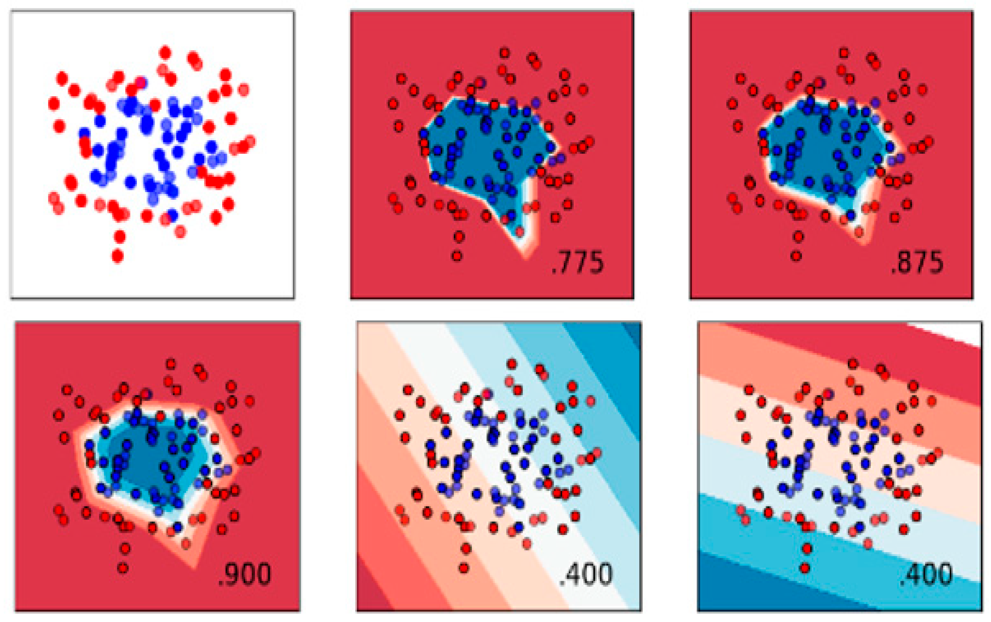
A multilayer perceptron regression model is a regression model used in machine learning, especially in antenna design for mapping parameters from one space to another, where each space can be of any number of dimensions. The multilayer perceptron regression model trains iteratively. The MLP optimizes the squared error using the stochastic gradient descent. The correlation coefficient was used as the evaluation paramtere for predicting the loss at each epoch. The rectified linear unit represents the max(0,x) whereas for the identity function as the activation unit f(x) = x is used.The activation function in the last layer is performed initially using the rectified linear unit as the activation function. Further, several other activation functions were tested, such as sigmoid and tangent. However, the identity function was found to be the best activation function integrated into the last layer. At each iteration, the loss function partial derivatives are computed to update the parameters. The L2 regularization term is set to 0.0001. it is further divided by the sample size after addition to the loss at each epoch. An adaptive learning rate of 0.001 is used, it is kept constant as long as the loss obtained at the taining is gradullay reced at each epoch, if not it is further reduced by dividing it by a factor of two. Further, the number of iterations are set to 200. The continuous values of output are obtained as the square error is used as the loss function. Weights with larger magnitudes are penalized using the L2 regularization function. The decision function for different values of alpha is given in Figure 5. These values are optimally obtained for the 60:40 train:test model, and maintained constant for the cross validation set-up.
3.3.2. Bayesian Additive Regression Tree (BART)
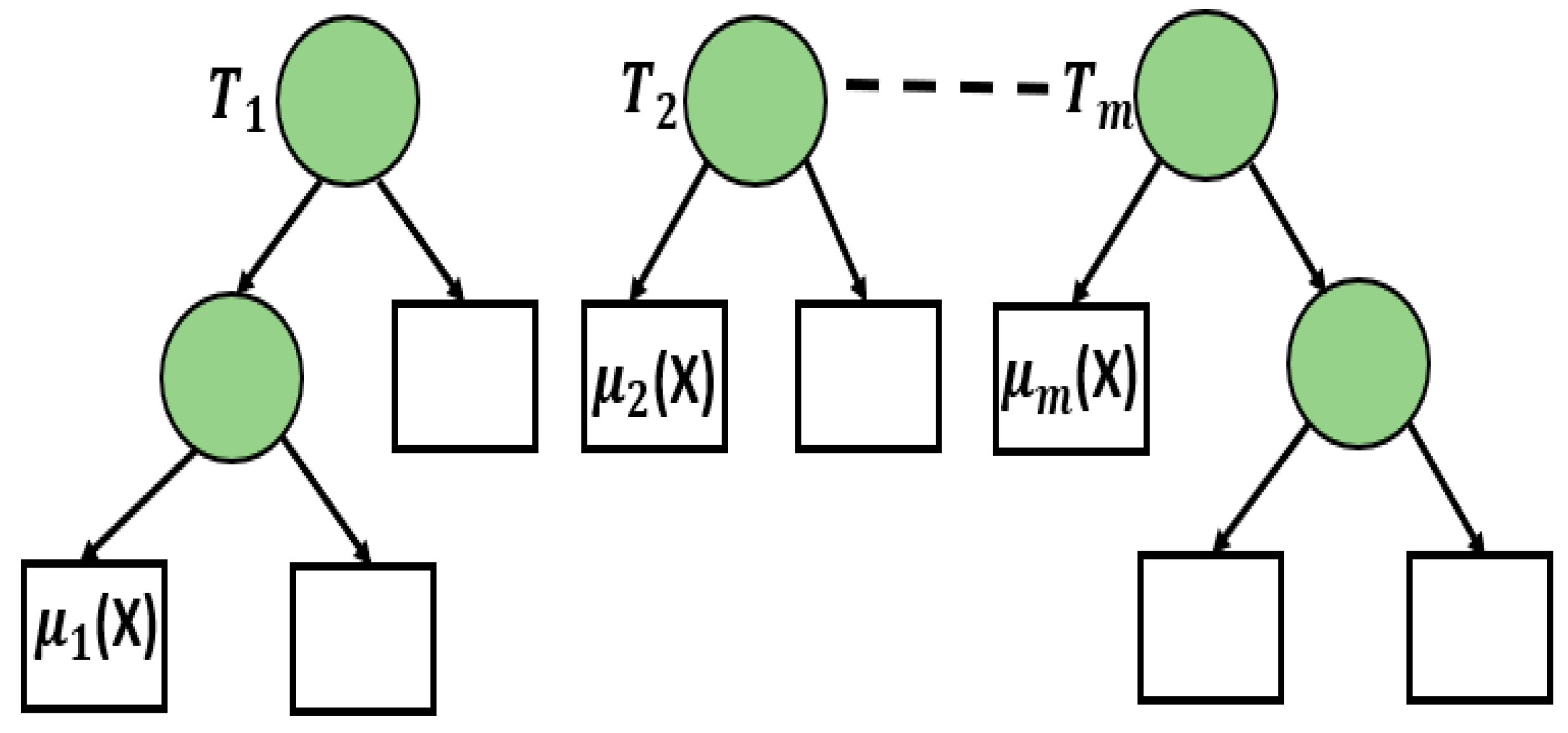
The BART technique is a bayesian ensemble technique that uses bayesian mechanisms to determine the posterior probabilities. The main reason for the BART to be Bayesian is the use of prior in contrast to the regression tress. The prior mimic the shallow trees with the value of the leaf tending towards zero. A good flexible approximation to the test set is obtained by fixing summation of several trees. Markov chain algorithm and back-fitting Monte Carlo algorithm is incorporated iteratively. The predictor space is partitioned into hyper triangles for approximation to an unknown function. The schematic representation of the BART model is shown in Figure 6. Mathematically, the BART model is represented as given in Equation (4).
3.3.3. AdaBoost of Decision Stump Trees
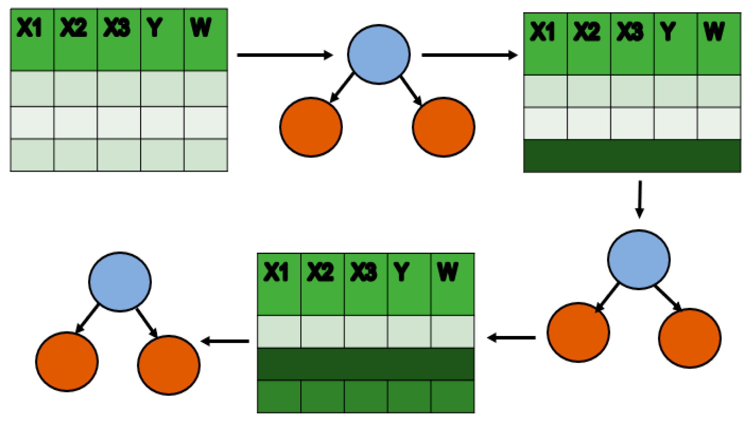
Decision trees with one level of a split are termed as decision stump trees. The main reasons for incorporating the ensemble model is to decrease the variance and bais, and further to improve the prediction rate. The weighted value of the sum of sample is always equal to one. Further, the actual influence of the stump over the entire ensemble is calculated. Considering misclassification error obtained during the traning, the value of alpha varies, a negative value indicates a strong disagreement between the predicted and the actal values, whereas a positive value indicates a strong agreement between the predicted and the actual value. Each time an ensemble model is created by considering the misclassified points with higher weightage. This involves multiple iterations to create a strong decision boundary for the weak learners. The learning rate hyper parameter is initially set to 0.01, for training the model. A smaller value of the learning rate increases the computational time for processing. The schematic representation of the decision stump tree model is shown in Figure 7.
3.3.4. Random Forest
Decision trees with bagging are trained using bootstrap aggregation. The initial step is random sampling with replacement performed for n instances in the dataset. In an individual tree, the number of features is chosen as three, and 20% of the variables are used in an individual run. Since there are three attributes a value lesser than three is selected to split the tree and the same value is held constant for the entire growth of the tree. The error rate relies on the strength of the correlation between the trees and the strength of each individual tree in the forest. A tree with a lower error rate is considered to be the strongest. The Algorithm 1, provides the pseudocode for generation of decision trees.
| Algorithm 1: Generate Decision Trees |
| Input: (Sample S,Features F) |
| 1.If stopping_condition(S,F) = true then |
| a.Leaf = createNode() b.leafLabel = classify(s) c.return leaf |
| 2. root = createNode() |
| 3. root.test_condition =findBestSpilt(S,F) |
| 4. V= {v | v a possible outcomecfroot.test_condition} |
| 5.For each value v Є V: a.= {s | root.test_condition(s) = v and s Є S }; b.Child = TreeGrowth ( ); c.Add child as descent of root and label the edge {root → child} as v 6.return root |
3.3.5. Decision Table
It is an accurate methodology in contrast to the decision trees, wherein an ordered set of If-then rules are used for numeric prediction. The decision trees are considered as a base. The number of attributes used is three consecutively, and the three rows are used for building the decision table. The goal of the decision table is to generate rules for structuring of the attributes. The same set of rules are further used ofr the cross validation set. The main rule formulated for our application is based on the distance of the query attribute to the attributes in the train set, the one with corresponsding to the least distance is choosen. The prediction is performed by allocating the newly arrived attribute to the category iteratively. The performance of the attribute is tested using the best subset of cross validation attributes. The best fit search strategy avoids the consequences of getting stuck in the best fit maxima and thus is adopted to search the attribute space [17].
3.3.6. Gaussain Regression
A set of a random variable with joint distribution are used in the Gaussian process [18]. In the gaussian regression, the prior value of the mean is taken as the mean value of the dataset. The hyperparameter optimization is performed by taking the maximum of log likelihood function. Further, subsequent iterations are conducted by taking the initial values of the parameters as described in the Algorithm 2. The process is completely specified by its covariance, variance, and mean functions. The algorithm for gaussian regression is as follows:
| Algorithm 2: Gaussain Regression |
| The dataset represented as |
| 1. Input: D=[xi,yi ],where 1<i<N x is the attribute, y is the prediction, N is the number of data points. x={length,width,frequency};y=S11 parameters |
| 2.Gaussian funxtion fitted to the data yi=f(xi )+€ϵN(0,σ2 ) € is the noise termin gaussian, ϵ is the Gaussian distribution Zero mean and variance is represented by |
| a.µ= |
| 3. kernels= Radial basis function, polynomial, normalized polynomial and Pearson VII |
| 4. V= Predicted value of the attribute |
3.3.7. Lazy BK
The objective function in the k nearest neighbor is computed using an estimation function. The lazy BK model as the name suggests is solely responsible for checking the outputs and properly packing the data values. The number of neighbors are controlled by identifying and validating the training dataset linearly as awell as quadratically. Due to this fact, the lazy BK is adopted even when the application varies [19]. The number of k nearest neighbors is predicted using the upper bound set as 2, or they can also be set depending on the best performance obtained through cross validation. Several distance measuring attributes are used, such as Chebyshev, Manhattan, Euclidean, and Minkowski. However, the best performance was obtained using Euclidean distance.
3.3.8. K-Star
The K-star algorithm uses a distance metric termed as entropy to compute the variation of the data, from the training set [20]. The entropy function is calculated using the mean value for transforming an instance to the other. The probability of this transformation occurs in a manner termed as “random walk. Here, for each class, a set of selected histogram features (dimensions and freqeuncy) are used as the input to the k-star model, and the missing values are replaced by the averge value of its corresponding neighbouring values. However, in our case there are no missing values in the dataset obtained from HFSS simulations. The regression result is computed by considering the sum of the probabilities with respect to the distance. The highest probability value is selected as the class or the variable value for the test attribute.
3.3.9. Locally Weighted Linear Regression (LWL)
The linear regression is a supervised algorithm for determining the linear relation between the predictor and the output [21,22]. The LWL assumes that the data are linear in nature; however, for a non-linear data as per our application the locally weigted regression model is employed. The total cost function is divided into multiple and smaller independent cost functions. Each datatpoint is treated as a weighting factor that expresses the influence of the datapoint over the predictions. The initial value of the cost function is as computed in Equation (5).
where x are the length, width, and frequency attributes, y is the S11 parameter. For each query, the value θ is computed. Higher priority or preference is given to the point belonging to the training set vicinity of the x, rather than far vicinity points. Based on this, the cost function J(θ) is modified as given in Equation (6).
The weight is generated for each query point using the exponential function. Thereby, it was inferred that the points belonging to the training set contributed significantly to the cost function rather than the points located in farther vicinity. The graph for the predicted fitting is given in Figure 6.
As it can observed from the Figure 8, a curvy regression line is used to fit the data value for the corresponding predictions.
3.3.10. Support Vector Regression
The classification model on par with the support vector machine, is a support vector regressor (SVR/RD). The SVR works towards finding the best hyperplane to separate the training data into its classes [23]. The best hyperplane that minimizes the cost function is chosen. Considering a batch size of 100 and a level set to minimal. A strict margin to draw the hyperplane is considered. The polynomial kernel is used as the kernel to fit the line to the data. The Figure 9 provides an illustration of the SMO to the regression problem. The ordinary least square method is used to determine the weight vector and the bias values such that the error or the loss function is minimal. The threshold allowance is set to 0.1, such that all the datapoints lying within the threshold allowance value are not penalized. Further, to compute the error the vertical distance between the plane and the points is used.
4. Results
The results of regression for the ten optimized regression models are computed using the following metrics.
4.1. Correlation Coefficient
The correlation coefficient (r) measures the degree of association between the predicted value and the true value. The range lies between −1 and +1. A value closer to 1 indicates a high degree of correlation between the two variables. The correlation coefficient is computed as given in Equation (7).
where, x and y represent the true and predicted values, respectively, SD represents standard deviation, and n represents the number of samples.
4.2. Mean Absolute Error (MAE)
The MAE metric gives a measure of error between the predicted and the true values and is computed for the entire dataset. The MAE is computed as given in Equation (8).
where, and y represent the true and predicted values, respectively, and represents the sample size.
4.3. Root Mean Squared Error (RMSE)
The root mean squared error gives the standard deviation of prediction errors. It gives the measure of the concentration of the data around the best line of fit. The RMSE is computed as given in Equation (9).
where, x and y represent the true and predicted values, respectively.
4.4. Relative Absolute Error and Root Relative Squared Error
The error metric is represented in the form of a ratio, defining the quantity of precision. The results of regression for 60:40 train and test attributes are given in Table 2.
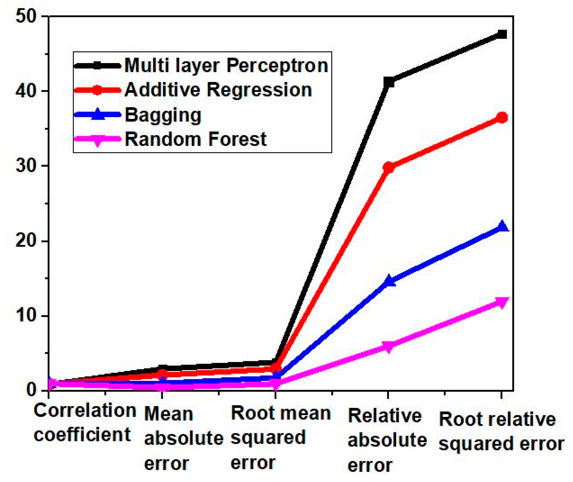
As it can be observed from Table 2, the random forest gives a good performance for correlation coefficient, MAE, RMSE, relative absolute error, and root relative squared error.
Similarly, as it can be observed from Table 3, Table 4 and Table 5, that optimized random forest gives a good performance for correlation coefficient, root relative squared error, MAE, RMSE, and relative absolute error for the ten-fold cross validation set-up. Figure 10, Figure 11, Figure 12 and Figure 13 gives a graphical illustration of the results for regression.
Nevertheless, it can be clearly observed from the graphical illustrations that a good performance for determining the S11 parameters of the antenna is obtained by employing a random forest classifier with a split size of two.
5. Conclusions
The proposed research work presented in the paper is an artificial intelligence-based approach to determine the antenna parameters for specific performance values. The antenna used for generating the datasets is simulated in HFSS and fabricated using an FR4 substrate. The simulated and experimental results coincide with one another. The feature selection mechanism resulted in a set of 3 features that exhibited a high degree of correlation between the feature and class and a lesser degree of correlation between them. An average correlation coefficient of 0.99 was obtained by using employing the proposed optimized random forest classifier. A heuristic approach was used for the selection of optimal parameters of random forest. The proposed system can be employed for predicting optimal values of the geometry of the composite structure UWB antenna that provides improved bandwidth.
Author Contributions
Conceptualization, S.P., P.K. (Praveen Kumar), T.A. and P.K. (Pradeep Kumar); methodology, S.P., P.K. (Praveen Kumar), T.A. and P.K. (Pradeep Kumar); software, S.P., P.K. (Praveen Kumar), T.A. and P.K. (Pradeep Kumar); validation, S.P., P.K. (Praveen Kumar), T.A. and P.K. (Pradeep Kumar); writing—original draft preparation, S.P.; writing—review and editing, S.P., P.K. (Praveen Kumar), T.A. and P.K. (Pradeep Kumar); supervision, T.A. All authors have read and agreed to the published version of the manuscript.
Funding
This research received no external funding.
Institutional Review Board Statement
Not Applicable.
Informed Consent Statement
Not Applicable.
Data Availability Statement
Data contained in the manuscript will be available on request to the readers.
Conflicts of Interest
The authors declare no conflict of interest.
References
- Suntives, A.; Hossain, M.S.; Ma, J.; Mittra, R.; Veremey, V. Application of artificial neural network models to linear and nonlinear RF circuit modeling. Int. J. RF Microw. Comput. Eng. 2001, 11, 231–247. [Google Scholar] [CrossRef]
- Liu, B.; Yang, H.; Lancaster, M.J. Global Optimization of Microwave Filters Based on a Surrogate Model-Assisted Evolutionary Algorithm. IEEE Trans. Microw. Theory Tech. 2017, 65, 1976–1985. [Google Scholar] [CrossRef] [Green Version]
- Zhang, X.; Tian, Y.; Zheng, X. Optimal design of fragment-type antenna structure based on PSO-CNN. In Proceedings of the International Applied Computational Electromagnetics Society Symposium (ACES), Miami, FL, USA, 14–18 April 2019; pp. 1–2. [Google Scholar]
- Calik, N.; Belen, M.A.; Mahouti, P. Deep learning base modified MLP model for precise scattering parameter prediction of capacitive feed antenna. Int. J. Numer. Model. Electron. Netw. Devices Fields 2019, 33, e2682. [Google Scholar] [CrossRef]
- Pan, G.; Wu, Y.; Yu, M.; Fu, L.; Li, H. Inverse Modeling for Filters Using a Regularized Deep Neural Network Approach. IEEE Microw. Wirel. Components Lett. 2020, 30, 457–460. [Google Scholar] [CrossRef]
- Wei, Z.; Liu, D.; Chen, X. Dominant-Current Deep Learning Scheme for Electrical Impedance Tomography. IEEE Trans. Biomed. Eng. 2019, 66, 2546–2555. [Google Scholar] [CrossRef] [PubMed]
- Zeng, M.; Nguyen, L.T.; Yu, B.; Mengshoel, O.J.; Zhu, J.; Wu, P.; Zhang, J. Convolutional Neural Networks for human activity recognition using mobile sensors. In Proceedings of the 6th International Conference on Mobile Computing, Applications and Services, Austin, TX, USA, 6–7 November 2014; pp. 197–205. [Google Scholar]
- Snoek, J.; Larochelle, H.; Adams, R. Practical Bayesian optimization of machine learning algorithms. Proc. Adv. Neural Inf. Process. Syst. 2012, 4, 1–9. [Google Scholar]
- Nan, J.; Xie, H.; Gao, M.; Song, Y.; Yang, W. Design of UWB Antenna Based on Improved Deep Belief Network and Extreme Learning Machine Surrogate Models. IEEE Access 2021, 9, 126541–126549. [Google Scholar] [CrossRef]
- Hinton, G.E.; Osindero, S.; Teh, Y.-W. A Fast Learning Algorithm for Deep Belief Nets. Neural Comput. 2006, 18, 1527–1554. [Google Scholar] [CrossRef] [PubMed]
- Mohamed, A.-R.; Dahl, G.E.; Hinton, G. Acoustic Modeling Using Deep Belief Networks. IEEE Trans. Audio Speech Lang. Process. 2011, 20, 14–22. [Google Scholar] [CrossRef]
- Mohamed, A.; Hinton, G. Deep belief networks for phone recognition. In Proceedings of the NIPS, Vancouver, Canada, 6–9 December 2010; p. 39. [Google Scholar]
- Abdel-Zaher, A.; Eldeib, A. Acoustic modeling using deep belief networks. Expert Syst. Appl. 2016, 46, 139–144. [Google Scholar] [CrossRef]
- Choi, E.; Chae, S.; Kim, J. Machine Learning-Based Fast Banknote Serial Number Recognition Using Knowledge Distillation and Bayesian Optimization. Sensors 2019, 19, 4218. [Google Scholar] [CrossRef] [PubMed] [Green Version]
- Shan, H.; Sun, Y.; Zhang, W.; Kudreyko, A.; Ren, L. Reliability Analysis of Power Distribution Network Based on PSO-DBN. IEEE Access 2020, 8, 224884–224894. [Google Scholar] [CrossRef]
- Balanis, C. Antenna Theory: Analysis and Design; John Wiley & Sons: Hoboken, NJ, USA, 2016. [Google Scholar]
- Kohavi, R. The power of decision tables. In Proceedings of the Machine Learning: ECML-95: 8th European Conference on Machine Learning Heraclion, Crete, Greece, 25–27 April 1995; Proceedings 8. Springer: Berlin/Heidelberg, Germany, 1995; pp. 174–189. [Google Scholar]
- Pillonetto, G.; Chiuso, A.; De Nicolao, G. Prediction error identification of linear systems: A nonparametric Gaussian regression approach. Automatica 2011, 47, 291–305. [Google Scholar] [CrossRef]
- Ali, P.J.M. Investigating the Impact of Min-Max Data Normalization on the Regression Performance of K-Nearest Neighbor with Different Similarity Measurements. ARO-THE Sci. J. KOYA Univ. 2022, 10, 85–91. [Google Scholar] [CrossRef]
- Painuli, S.; Elangovan, M.; Sugumaran, V. Tool condition monitoring using K-star algorithm. Expert Syst. Appl. 2014, 41, 2638–2643. [Google Scholar] [CrossRef]
- Özçift, A. Forward stage-wise ensemble regression algorithm to improve base regressors prediction ability: An empirical study. Expert Syst. 2014, 31, 1–8. [Google Scholar] [CrossRef]
- Rajendran, S.; Ayyasamy, B. Short-term traffic prediction model for urban transportation using structure pattern and regression: An Indian context. SN Appl. Sci. 2020, 2, 1–11. [Google Scholar] [CrossRef]
- Mohammed, D.Y. The web-based behavior of online learning: An evaluation of different countries during the COVID-19 pandemic. Adv. Mob. Learn. Educ. Res. 2022, 2, 263–267. [Google Scholar] [CrossRef]
Figure 1.
UWB antenna (a) UWB structure simulated in HFSS front and ground plane. (b) Prototype of UWB antenna (c) simulated and measured reflection coefficient of the UWB antenna.
Figure 1.
UWB antenna (a) UWB structure simulated in HFSS front and ground plane. (b) Prototype of UWB antenna (c) simulated and measured reflection coefficient of the UWB antenna.

Figure 2.
Ground plane analysis.

Figure 3.
Radiating structure analysis to achieve UWB frequency range.

Figure 4.
Stepwise regression methodology.

Figure 5.
Illustration of decision function for various alpha values: First Row (left to Right), Data distribution, for alpha = 0.15, and for alpha = 0.33, Second Row (left to Right), for alpha = 1.00, for alpha = 3.16, and for alpha = 10.00.
Figure 5.
Illustration of decision function for various alpha values: First Row (left to Right), Data distribution, for alpha = 0.15, and for alpha = 0.33, Second Row (left to Right), for alpha = 1.00, for alpha = 3.16, and for alpha = 10.00.

Figure 6.
Illustration of BART model.

Figure 7.
Illustration of decision stump tree model.

Figure 8.
Illustration of linear regression model fit to data.

Figure 9.
Illustration of SVR model for the regression problem.

Figure 10.
Results of regression for 60:40 model.

Figure 11.
Results of regression for ten fold-cross validation model.

Figure 12.
Results of regression for the 60:40 model.

Figure 13.
Results of regression for ten fold-cross validation model.


Table 1.
Optimized physical parameters of the proposed UWB antenna (dimensions are in mm).
| Parameters/Antenna Design | WS | LS | Z1 | Z2 | Z3 | Z4 | Z5 | Z6 | Z7 | Z8 | Z9 |
|---|---|---|---|---|---|---|---|---|---|---|---|
| UWB | 21.5 | 17 | 2 | 5.6 | 2.4 | 2.7 | 7 | 3.8 | 2 | 7.3 | 4 |
Table 2.
Regression results for 60:40 split.
| Evaluation Parameters | Multilayer Perceptron | Additive Regression | Bagging | Random Forest |
|---|---|---|---|---|
| Correlation coefficient | 0.88 | 0.93 | 0.97 | 0.99 |
| Mean absolute error | 2.95 | 2.13 | 1.04 | 0.43 |
| Root mean squared error | 3.84 | 2.94 | 1.76 | 0.96 |
| Relative absolute error | 41.40 | 29.86 | 14.6 | 6.01 |
| Root relative squared error | 47.73 | 36.54 | 21.88 | 11.97 |
Table 3.
Regression results for ten-fold cross validation.
| Evaluation Parameters | Multilayer Perceptron | Additive Regression | Bagging | Random Forest |
|---|---|---|---|---|
| Correlation coefficient | 0.89 | 0.91 | 0.96 | 0.98 |
| Mean absolute error | 2.54 | 2.29 | 0.94 | 0.47 |
| Root mean squared error | 3.81 | 3.39 | 2.05 | 1.28 |
| Relative absolute error | 34.23 | 30.89 | 12.69 | 6.35 |
| Root relative squared error | 45.18 | 40.26 | 24.39 | 15.28 |
Table 4.
Regression results for 60:40 split.
| Evaluation Parameters | Decision Table | Gaussian | Lazy BK | K Star | LWL | SVR |
|---|---|---|---|---|---|---|
| Correlation coefficient | 0.88 | 0.88 | 0.97 | 0.95 | 0.88 | 0.94 |
| Mean absolute error | 2.36 | 2.95 | 0.66 | 1.97 | 3.11 | 1.75 |
| Root mean squared error | 3.71 | 3.84 | 1.76 | 3.05 | 4.35 | 2.89 |
| Relative absolute error | 33.06 | 41.4 | 9.35 | 27.6 | 43.26 | 24.5 |
| Root relative squared error | 46.15 | 47.73 | 21.8 | 37.9 | 54.07 | 35.9 |
Table 5.
Regression Results for ten fold-cross validation.
| Evaluation Parameters | Decision Table | Gaussian | Lazy BK | K Star | LWL | SVR |
|---|---|---|---|---|---|---|
| Correlation coefficient | 0.83 | 0.78 | 0.87 | 0.85 | 0.86 | 0.95 |
| Mean absolute error | 2.35 | 1.95 | 0.56 | 1.77 | 3.10 | 165 |
| Root mean squared error | 3.60 | 2.84 | 0.99 | 2.05 | 4.30 | 2.59 |
| Relative absolute error | 31.6 | 39.4 | 8.35 | 26.6 | 42.2 | 22.5 |
| Root relative squared error | 45.15 | 45.73 | 20.8 | 36.9 | 53.0 | 34.9 |
Disclaimer/Publisher’s Note: The statements, opinions and data contained in all publications are solely those of the individual author(s) and contributor(s) and not of MDPI and/or the editor(s). MDPI and/or the editor(s) disclaim responsibility for any injury to people or property resulting from any ideas, methods, instructions or products referred to in the content. |
© 2023 by the authors. Licensee MDPI, Basel, Switzerland. This article is an open access article distributed under the terms and conditions of the Creative Commons Attribution (CC BY) license (https://creativecommons.org/licenses/by/4.0/).
Share and Cite
MDPI and ACS Style
Pathan, S.; Kumar, P.; Ali, T.; Kumar, P. Automated and Optimized Regression Model for UWB Antenna Design. J. Sens. Actuator Netw. 2023, 12, 23. https://doi.org/10.3390/jsan12020023
AMA Style
Pathan S, Kumar P, Ali T, Kumar P. Automated and Optimized Regression Model for UWB Antenna Design. Journal of Sensor and Actuator Networks. 2023; 12(2):23. https://doi.org/10.3390/jsan12020023
Chicago/Turabian StylePathan, Sameena, Praveen Kumar, Tanweer Ali, and Pradeep Kumar. 2023. "Automated and Optimized Regression Model for UWB Antenna Design" Journal of Sensor and Actuator Networks 12, no. 2: 23. https://doi.org/10.3390/jsan12020023
Note that from the first issue of 2016, this journal uses article numbers instead of page numbers. See further details here.