Recursive Feature Elimination with Cross-Validation with Decision Tree: Feature Selection Method for Machine Learning-Based Intrusion Detection Systems

Abstract

The frequency of cyber-attacks on the Internet of Things (IoT) networks has significantly increased in recent years. Anomaly-based network intrusion detection systems (NIDSs) offer an additional layer of network protection by detecting and reporting the infamous zero-day attacks. However, the efficiency of real-time detection systems relies on several factors, including the number of features utilized to make a prediction. Thus, minimizing them is crucial as it implies faster prediction and lower storage space. This paper utilizes recursive feature elimination with cross-validation using a decision tree model as an estimator (DT-RFECV) to select an optimal subset of 15 of UNSW-NB15’s 42 features and evaluates them using several ML classifiers, including tree-based ones, such as random forest. The proposed NIDS exhibits an accurate prediction model for network flow with a binary classification accuracy of 95.30% compared to 95.56% when using the entire feature set. The reported scores are comparable to those attained by the state-of-the-art systems despite decreasing the number of utilized features by about 65%.

1. Introduction

The recent advancements in technology have resulted in the emergence of various innovative concepts, including the Internet of Things (IoT). IoT networks are composed of a vast array of Internet-connected systems and sensors. Per the International Data Corporation (IDC), it is estimated that by 2025, the number of IoT devices connected to the Internet will surpass 41 billion [1]. The rise of IoT and its extensive connectivity capability had a positive impact on several domains including industry, transport, environment, and power management [2]. On the other hand, the massive amount of data exchanged over IoT networks poses concerns to the confidentiality, integrity, and availability of the interconnected systems. These networks provide an ideal ground for potential attackers to launch cyberattacks, compromising systems’ security [3,4]. Due to the high stakes, there is an urgent need for an accurate and reliable network intrusion detection system (NIDS) that is also capable of identifying zero-day attacks. Anomaly-based NIDS can achieve that by creating a profile of typical network behavior and flagging any deviations as potential attacks. Anomaly-based NIDSs can leverage various artificial intelligence (AI) techniques, including supervised and unsupervised methods [5].

In this study, we utilize a recently world-renowned dataset known as UNSW-NB15. This dataset was created to overcome the drawbacks of previous datasets, such as the undistributed and outdated KDD98, NSL-KDD, and KDDCUP99 [6,7]. Our aim is to conduct binary classification via part of the dataset’s 49 features. By minimizing the number of employed features, we can improve detection time, storage requirements, and overall operational efficiency of networks. However, reducing the number of features may result in a trade-off with prediction accuracy. Thus, we sought to find the right balance in feature selection. Our research aims to effectively classify network data records as either standard or malicious classes using only 15 features. Those features were determined using the recursive feature elimination (RFE) algorithm [8]. The accuracy of the chosen features was evaluated using six machine learning classifiers: Logistic Regression (LR) [9], Naïve Bayes (NB) [10], Stochastic Gradient Descent [11], Random Forest (RF) [12], AdaBoost [13], and Multi-layer Perceptron [14].

The complete UNSW-NB15 dataset comprises 49 features and a total of around 2.5 million data rows, with each row classified into either benign (normal) or one of nine possible attacks (Analysis, Backdoor, DoS, Exploits, Fuzzers, Generic, Reconnaissance, Shellcode, and Worms). In our research, we utilized the publicly available testing and training sets, which comprise about 10% of the dataset (257,673 records and 42 features including 175,341 records used for training and 82,332 records used for testing). An elaborate description of the dataset is provided in the upcoming sections.

While previous research has achieved remarkable accuracy with extensive feature sets, our objective was to minimize the number of features while maintaining a detection system that remains highly accurate. Fewer features result in faster prediction times, lower storage requirements, and improved operational efficiency.

A summary of our research contributions to the literature and findings are listed below:

• An overview of the intrusion detection problem in the UNSW-NB15 dataset, highlighting the importance and challenges associated with this specific dataset.
• A detailed literature review of existing NIDSs and their limitations and shortcomings, focusing on those that adopted the recursive feature elimination (RFE) method and those that utilized UNSW-NB15.
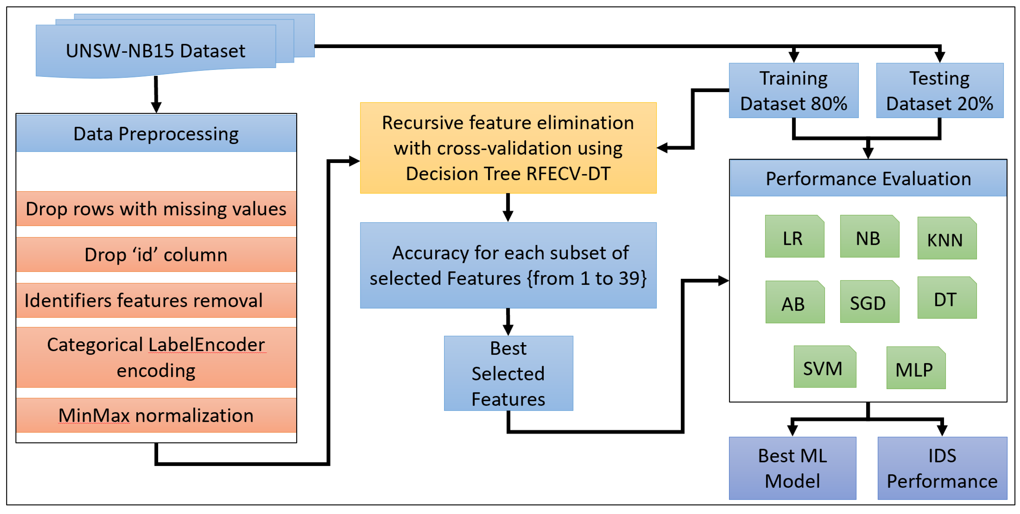
• Proposed a recursive feature elimination with cross-validation (RFECV) approach using binary decision tree classification for machine learning-based intrusion detection systems.
• Generated an optimal set of features selected from the UNSW-NB15 dataset using RFECV with a decision tree model as the estimator. Then, we evaluated their performance prediction capability via multiple well-known machine learning classifier models.
• Applied data preprocessing techniques on the UNSW-NB15 dataset to address overfitting and biasing issues. This included removing duplicate rows and eliminating identifier features such as IP and port-related features and TTL-based features that were deemed unrealistically correlated with the label features and could cause bias.
• Experimental findings using the UNSW-NB15 dataset demonstrated that the proposed model reduced the feature dimension from 42 to 15 while gaining a prediction accuracy of 95.30% compared to 95.56% with the original dataset and maintaining a similar F1-score (95.29% compared to 95.55%).

The rest of this paper is structured as follows: Section 2 explores the literature, Section 3 presents the methodology, Section 4 explains the results and analysis, and Section 5 concludes the paper and sheds light on future work directions.

2. Related Work

UNSW-NB15 is an intrusion network dataset that researchers have widely utilized in recent years. The research interest varied based on the work objective [15,16,17,18]. This section presents relevant intrusion detection systems that used UNSW-NB15 and reports their results. Additionally, this section sheds light on the use of RFE in feature selection for intrusion detection.

In [19], Yin et al. proposed an anomaly-based network intrusion detection system utilizing UNSW-NB15. Their feature selection process consisted of two stages. In the first stage, they applied information gain followed by random forest to eliminate less important features. In the second stage, the authors employed RFE with an MLP classifier to reduce the number of features further down to 23 features. Yin et al. proposed a multiclassification model that resulted in %84.24 accuracy and %82.85 F1-score.

In [20], Alissa et al. utilized 34 features from the partial UNSW-NB15 dataset and performed binary classification. The authors tested their model using several classifiers: decision tree, XGB, and Logistic Regression. The decision tree classifier outperformed the others with an accuracy of 94%. Likewise, the F-1 score, recall, and precision resulted in a similar score.

In [21], the authors combined Grey Wolf Optimizer and Bald Eagle Search to select the best 31 features. The classification was achieved using Deep Sparse Auto-Encoder (DSAE). Mulyanto et al. reported an accuracy, F-1 score, recall, and precision above 99%.

In another study, Tama et al. [22] selected 19 UNSW-NB15 features using particle swarm optimization (PSO) and achieved 91.27% accuracy and 91.44% F1-score using a combined Rotation Forest and Bagging classifier. During their work on the partial dataset, the authors also tried Ant Colony Optimization (ACO) and Genetic Algorithm (GA) for feature selection. However, PSO’s chosen features showed the best results.

Nawir et al. [23] attempted to differentiate between benign and malicious network flows using the entire dataset, including all 42 features. The authors experimented with three classifiers: Average One Dependence Estimator (AODE), Naive Bayes (NB), and Bayesian Network (BN) and reported the highest accuracy of 94.37% using AODE.

In a recent study [24], Thakkar and Lohiya employed statistical importance to select 21 features. The authors utilized deep neural networks (DNNs) to predict network traffic. The study resulted in 89.03% accuracy and an F1-score of 96.93%. Liu and Shi also employed deep neural networks in their classification [25]. However, they extracted 30 features using the genetic algorithm. Liu and Shi reported an accuracy of 76.70% and an F1-score of 93.83%. A DNN was employed by another study but as a feature selection method. Eunice et al. fed the twenty chosen features into a random forest model, achieving 82.1% accuracy [26].

Barkah et al. [27] utilized UNSW-NB15 and conducted several experiments to determine the best detection model. In one of the scenarios, RFE was used to choose the best 13 features. The selected features were fed to four classifiers. Random forest and decision tree exhibited the best multiclassification results, whereas RF scored an accuracy of 85.07% and an F1-score of 85.68%, while DT resulted in 85.64% accuracy and an F1-score of 86.87%. Their results were similar (or lower) in other scenarios where they attempted to handle imbalanced data using oversampling and adaptive synthetic techniques.

In another study, Kumar et al. utilized the UNSW-NB15 dataset to build their multiclass detection model [28]. The authors applied Information Gain to select 13 features. The model resulted in an accuracy of 83.84% and was later used to assess a real-time generated dataset with a reported accuracy of 83.8%.

Kasongo and Sun [29] opted for XGBoost to extract 19 features from the UNSW-NB15 dataset. They achieved 90.85% accuracy and 88.45% F1-score using the Decision Tree (DT) classifier. In another study [30], the authors employed an enhanced Pigeon Inspired Optimizer (PIO) version to select five UNSW-NB15 features (dstip, dsport, sbytes, sloss, and stime). The authors reported an accuracy of 91.7% and 90.9% F1-score. However, it is essential to highlight that the five chosen features included two destination-related features for the port and IP addresses (dstip and dsport). Typically, these features and timestamps-related ones, such as stime, are dropped in the preprocessing phase to avoid learning bias [31].

Sarhan et al. investigated the usability of UNSW-NB15 in the network security domain [32]. One of their observations was the biased prediction results when including any Time-to-Live (TTL)-based features, namely sttl, dttl, and ct_state_ttl. In their work, and due to the high correlation between these features and the outcome labels, they referred to the TTL features as “hidden labels”. In their opinion, the high predictive powers of these features relate to the dataset’s testbed design issues. Thus, we opted to exclude these three features from our experiments. However, and to the best of our knowledge, none of the related work followed a similar approach. In fact, some [15,16] deemed the sttl feature to be highly efficient [32]. Likewise, as mentioned earlier, it is essential in artificial datasets to drop features that may result in a bias toward a specific victim or attacking nodes. Thus, identifying characteristics related to IP and port source/destination and timestamps are usually dropped. Therefore, we excluded srcip, sport, dstip, dsport, stime, and ltime in our research.

Many researchers investigated using RFE as a wrapper method, either by itself or combined with another selection method, to reduce the feature subset. For example, Megantara et al. combined RFE and Gini importance to determine the most suitable features for detecting multiclass attacks in the NSL-KDD dataset [33]. In [34], the authors utilized RFE to find the most suitable four features to predict attacks in CICIDS2017. Their Multi-layer Perceptron classifier resulted in an accuracy of 89%. Sharma et al. [35] also employed RFE to find the best features to detect multiclass attacks in the KDD CUP99 dataset. The authors tested their features using several models, including decision tree and support vector machine (SVM), and reported a reasonable classification rate. In another study, Tonni et al. [36] used RFE to select a subset of CSE-CIC-IDS-2018 features and then verified their model using random forest.

Lastly, two recent studies [37,38] applied Recursive Feature Elimination over CSE-CIC-IDS2018. In [37], Ren et al. reduced about 80% of the dataset features before implementing deep reinforcement learning to detect anomalies. Alahmed et al. used RFE and principal component analysis (PCA) on the same dataset [38].

3. Proposed Methodology

This section illustrates the research methodology’s architectural framework, beginning with the proposed system’s architecture. As Figure 1 shows, the proposed system comprises three primary blocks: Data Preprocessing, Features Selection, and Classification.

3.1. Data Preprocessing

Data processing, known as data engineering, plays a vital role in the success of the learning process. Data processing consists of Columns and Rows Cleaning, Features Encoding, and Data Normalization.This subsection discusses the procedures applied in the preprocessing phase, which aims to adequately prepare the data for analysis.

3.1.1. Drop Rows with Missing Values

All rows were examined to identify any missing values. Since the partitioned 10% dataset used in this research has been processed, no missing values were detected except for the “service” feature. We decide to retain this feature in its current state, as it signifies the absence of service. It will be encoded later during the encoding phase.

3.1.2. Drop id Column

Dropping the “id” column is a common step in data preprocessing because it does not provide any meaningful information. Removing the “id” column ensures that only relevant features are considered for further analysis. It is important to mention that the 10% dataset did not include any features related to port and IP addresses, as well as timestamps, which are considered identifiers.

3.1.3. Identifiers Features Removal

As raised by Sarhan et al. and reported by others [32,39], the inclusion of the TTL-based features “sttl”, “dttl”, and “ct_state_ttl” in the UNSW-NB15 dataset could introduce bias during the classification process and impact the reliability of classifier evaluation. These features are considered unrealistically highly correlated to “Label”. For this reason, these features were removed from the dataset to ensure a more accurate and unbiased analysis. Consequently, the number of features were reduced from 42 to 39 features. As mentioned earlier, the 42 features do not include other identifiers, such as those related to IP and port source/destination and timestamps.

3.1.4. Categorical LabelEncoder Encoding

Categorical transformation is important for improving the learning capability of classifiers that can only process numeric values. In the case of the used UNSW-NB15 dataset, the features “proto”, “service”, and “state” contain categorical data that have been encoded into numerical values.

As encoding techniques, we have decided to use LabelEncoder [40]. It is suitable with the UNSW_NB15 dataset as it assigns a unique numerical label to each unique categorical value. This transformation allows the classifier to interpret and learn from the encoded labels. Although LabelEncoder does not create separate binary columns like OneHotEncoder, it still captures the categorical nature of the feature [41].

The “service” feature contains 13 categorical values, such as [‘-’ (unknown), ‘ftp’, ‘smtp’, ‘snmp’, ‘http’, ‘ftp-data’, ‘dns’, ‘ssh’, ‘radius’, ‘pop3’, ‘dhcp’, ‘ssl’, and ‘irc’]. These categorical values have been encoded into numbers ranging from 0 to 12. Similarly, the “state” feature contains nine categorical values, namely [‘FIN’, ‘INT’, ‘CON’, ‘ECO’, ‘REQ’, ‘RST’, ‘PAR’, ‘URN’, and ‘no’], which are encoded into numbers from 0 to 8. Lastly, the “proto” feature contains 128 categorical values that are encoded into numbers from 0 to 127.

3.1.5. MinMax Normalization

The presence of high numerical values in different features affects the learning process of machine learning classifiers such as LR, NB, SVM, SGD, and MLP. Additionally, training high-dimensional datasets requires significant computational resources. To address these issues, various normalization methods, such as Min-Max Normalization, Z-score Normalization, Decimal Scaling, or Max normalization could be used [42]. The choice of method typically depends on the application. In this step, Min-Max scaling was applied on the dataset using Equation (1).

$$X_{\mathrm{scaled}}=\frac{X-X_{\min }}{X_{\max }-X_{\min }}$$

(1)

This scaling technique mapped the original values to a range between 0 and 1, preserving the relative relationships among the data points.

It is important to note that normalization was not applied during the feature selection phase, as the decision tree (DT) model used in this phase is not sensitive to high numerical values of features. However, the training and testing datasets used to train the machine learning classifiers were normalized to ensure accurate and reliable model performance.

Additional details about UNSW-NB15 are provided in the upcoming sections.

3.2. RFECV Using DT for Features Selection

To perform feature selection, a DT-REFCV method is applied on the processed data, which generates the best-selected features based on their importance scores. This subsection illustrates how the features were chosen using recursive feature elimination.

3.2.1. Decision Tree

A Decision Tree (DT) is a supervised ML technique widely used for classification and regression tasks. DT depicts a tree-like structure wherein the internal nodes represent the features, while leaf nodes comprise the class labels or predicted values. Thus, a prediction is made by traversing the path from the root to one of the leaf nodes depending on the input’s feature values.

A decision tree makes predictions by following a sequence of if-else conditions, as  represented in Equation (2) [43]:

$$F\left(x\right)=\left\{\begin{array}{cc}{C}_1,\hfill & \mathrm{if}x\in S_1\hfill \\ C_2,\hfill & \mathrm{if}x\in S_2\hfill \\ \dots \hfill \\ C_k,\hfill & \mathrm{if}x\in S_k\hfill \end{array}\right.$$

(2)

where $F\left(x\right)$ is the final prediction, $C_i$ is the class label or predicted value for input subset $S_i$, and x depicts the input. The input subsets $S_i$ are defined by the tree’s decision boundaries.

Decision trees are easy to comprehend and interpret, as the decision rules can be visualized. DTs can handle numerical and categorical features and are robust to outliers and missing values. Additionally, DTs can capture complex nonlinear relationships within the data with simple preprocessing. DTs are also utilized for feature selection, as they assign importance scores to the attributes based on their contribution to the decision-making process.

Decision tree is a powerful technique that has been employed in numerous fields, including machine learning, image processing, and pattern identification. Furthermore, it has been used in various applications across different disciplines.

There are various types of DT algorithms, including ID3, C4.5, CART, CHAID, MARS, GUIDE, CTREE, CRUISE, and QUEST [43]. In our study, we used the CART algorithm, which is the default DT algorithm implemented in the scikit-learn library.

The DT algorithms have different characteristics and are suitable for various data types and tasks. Each algorithm has its benefits and can be applied depending on the problem’s requirements. For example, some algorithms, like ID3 and C4.5, use entropy and information gain for tree construction [44], while others, such as CART and CHAID, use impurity measures like Gini index or chi-squared tests [45]. MARS employs piecewise linear functions instead of binary splits, while GUIDE and CTREE focus on detecting interactions [46]. CRUISE and QUEST use statistical tests for partitioning.

3.2.2. Recursive Feature Elimination with Cross-Validation

RFECV is a wrapper feature selection method that uses a machine learning algorithm to select the most relevant features for the intrusion detection problem. To ensure its robustness, RFECV combines recursive feature elimination and cross-validation to identify the optimal number of features that maximize the performance of the model [8].

RFECV uses a classification machine learning model to score each feature and iteratively eliminates features that do not enhance the classification accuracy. As outlined in Algorithm 1, the feature search process uses backward selection, beginning with the complete feature set and progressively removing features that do not contribute to the accuracy of classification, ultimately identifying the most effective feature subset. In this research work, the implementation of RFECV was conducted using the decision tree classification model DT-RFECV as an estimator and the fold (k) for cross-validation equal to 10 with StratifiedKFold as splitting strategy to preserve the percentage of samples for each class. With 10-fold cross-validation, the dataset was split into 10 equal-sized folds.

Algorithm 1 RFECV with DT

Require: Training set X Ensure: Ranked features   1: for all features in X do   2:       for $k=1$ to 10 do                                                      ▹k is the number of folds for   3: cross-validation.   4:             X is randomly divided into ten equal subsets   5: using StratifiedKFold method;   6:             One subset is used as validation data, and the   7: remaining nine subsets are used as training data;   8:             Train a DT model using the training data;   9:             Calculate the prediction accuracy using the validation data; 10:             Obtain the weight of each feature produced by the DT model; 11:             Drop l least weighted features and update the training data; 12:       end for 13:   14:       Obtain the feature subset $FS$ with the highest prediction accuracy; 15:       if prediction accuracy of $FS$ is the highest then 16:             Selected features = $FS$; 17:       end if 18: end for 19: Return ranked selected features.

During the recursive elimination process, as features are eliminated in a recursive manner, the accuracy metric is calculated at each iteration for evaluating the impact of feature elimination on the model performance. By observing how the accuracy metrics change with each iteration, insights can be gained regarding the importance and contribution of each feature to the model’s performance. The optimal feature set was determined by the classifier with the highest overall accuracy.

After the recursive elimination process is completed, the selected set of features is evaluated using 10-fold cross-validation. Subsequently, the DT model is repeatedly trained and evaluated (ten times), each time using a distinct fold as the validation set and the remaining folds serve as the training set. The accuracy metrics were used to estimate how well the model generalizes to unseen data and helps in evaluating DT model robustness. The average and standard deviation of the accuracy metrics across the 10 iterations are calculated to provide a thorough evaluation of the model’s performance.

For each iteration of the cross-validation process, the RFE process calculates internal accuracy metrics to evaluate the performance of feature selection. It helps in assessing the effectiveness of the selected features in classifying attack and non-attack classes.

It is important to emphasize that the accuracy values utilized to identify the model with the highest accuracy within each training sample set were determined based on the final accuracy assessment using the test dataset. These accuracy values were not derived from the inner accuracy metrics calculated during the RFE execution and the 10-fold cross-validation tuning [8].

3.3. Classification Using Machine Learning Algorithms

Once the best features are selected, several machine learning classification models are trained using the training set. Then, the performances of the trained models are evaluated using the test dataset. This step exhibits the best performing machine learning based IDS. As stated earlier, machine learning plays a pivotal role in predicting network anomalies, which is a main priority for network intrusion detection systems. This subsection presents and describes six well-known classifiers utilized in our study.

3.3.1. Logistic Regression

Despite the name’s insinuation, logistic regression (LR) is a machine learning technique commonly used for binary classification tasks. Additionally, LR can also be extended to handle multi-classification tasks using the one-vs-rest method. The LR model applies the sigmoid function or its variations to a linear machine learning model. This transformation confines the output values within the range of [0, 1]. A value closer to 1 signifies a higher probability of belonging to a particular class. Equations (3) and (4) provide the mathematical formulation of LR [9].

$$h_{\beta }\left(x\right)={\beta }_0+{\beta }_1{x}_1+{\beta }_2{x}_2+\dots +{\beta }_n{x}_n$$

(3)

$$P(y=1\mid x)=\frac{1}{1+e^{-h_{\beta }\left(x\right)}}$$

(4)

Equation (3) represents the linear combination of the input features $x_1,x_2,\dots ,x_n$ and their corresponding coefficients ${\beta }_0,{\beta }_1,{\beta }_2,\dots ,{\beta }_n$. This linear combination is used as an input to the sigmoid function.

The sigmoid function denoted by $e^{-h_{\beta }\left(x\right)}$, transforms the linear combination into a probability value between 0 and 1. The final Equation (4) $(y=1\mid x)$ represents the probability of the binary outcome y being 1 given the input variables x.

3.3.2. Naive Bayes

Naive Bayes (NB) is a probabilistic classification algorithm based on Bayes’ theorem and presumes that the features are conditionally independent of the class [10]. NB is suited for binary classification problems. By evaluating the input features, NB computes the probability of each class and chooses the one with the most significant likelihood, as depicted in Equation (5):

$$P\left(C_k\right|x_1,x_2,\dots ,x_n)=\frac{P\left(C_k\right){\prod }_{i=1}^{n}P\left(x_i\right|C_k)}{P(x_1,x_2,\dots ,x_n)}$$

(5)

where $P\left(C_k\right|x_1,x_2,\dots ,x_n)$ is the posterior probability of class $C_k$ given the input features $x_1,x_2,\dots ,x_n$, $P\left(C_k\right)$ is the prior probability of class $C_k$, $P\left(x_i\right|C_k)$ is the likelihood of feature $x_i$ given class $C_k$, and $P(x_1,x_2,\dots ,x_n)$ is the probability of the input features. The classifier chooses the class with the highest posterior probability [10].

Despite its straightforward approach, Naive Bayes has achieved promising results in diverse domains, such as text classification, spam filtering, and sentiment analysis.

3.3.3. Stochastic Gradient Descent

Stochastic gradient descent (SGD) is an iterative optimization algorithm that has also been widely utilized in training machine learning models [11]. SGD can efficiently update the model’s parameters incrementally, making it extremely suitable for large-scale datasets. SGD updates the model parameters by taking small steps toward the negative gradient of the loss function with respect to the parameters. The update rule for each parameter ${\theta }_j$ is represented in Equation (6):

$${\theta }_j^{(t+1)}={\theta }_j^{\left(t\right)}-\eta \frac{\partial L}{\partial {\theta }_j}$$

(6)

where ${\theta }_j^{(t+1)}$ is the updated value of parameter ${\theta }_j$ at iteration $t+1$, $\eta$ is the learning rate that controls the step size, and $\frac{\partial L}{\partial {\theta }_j}$ is the gradient of the loss function with respect to ${\theta }_j$. The gradients are commonly estimated using a randomly selected subset of the training data, commonly known as mini-batch, to reduce computational cost. SGD iteratively performs these parameter updates until convergence or a predefined number of iterations.

Although it is susceptible to noisy updates, SGD shows fast convergence and can handle large datasets efficiently, making it a popular choice for training a variety of machine learning models.

3.3.4. Random Forest

Random forest (RF) is an ensemble learning technique that merges several decision trees to create a robust and accurate model. It performs by creating multiple decision trees during training and predicts the class based on the most frequent class predicted by the individual trees. Each decision tree in the forest is trained on a different subset of the training data, and the final prediction is determined by a voting method based on the predictions of all the trees [12]. The prediction of a random forest model is represented in Equation (7):

$$F\left(x\right)=\frac{1}{N}\sum _{i=1}^N{f}_i\left(x\right)$$

(7)

where $F\left(x\right)$ is the final prediction, N is the number of decision trees in the forest, and $f_i\left(x\right)$ is the prediction of the ith decision tree. The RF algorithm introduces randomness in two ways. Firstly, by unsystematically selecting subsets of the features for each tree. Then, by bootstrapping the training data after determining the number of trees to build, allowing each tree to be trained on a different data subset. Such randomness reduces overfitting and improves the model’s generalizability and robustness.

Random forest models apply to both classification and regression tasks. RF is capable of handling large datasets with high-dimensional feature spaces and is resistant to overfitting. Additionally, it provides estimates of feature importance, allowing for feature selection. Furthermore, RF can capture complex relationships and interactions between features, making it a popular choice in various domains. However, it may be sensitive to noisy data and can be computationally demanding when training large forests.

3.3.5. AdaBoost

Adaptive Boosting (AdaBoost) is an ensemble learning method that merges multiple classifiers to produce a robust classifier [13]. It works by iteratively training learners on different weighted subsets of the training data. The algorithm assigns higher weights to misclassified samples. The final prediction is determined by a weighted mixture of the weak learners’ predictions. The weight of each weak learner is determined by its performance in classifying the training examples. The prediction of the AdaBoost model is computed using Equation (8):

$$F\left(x\right)=\sum _{t=1}^T{\alpha }_t{h}_t\left(x\right)$$

(8)

where $F\left(x\right)$ denotes the final prediction, T is the number of weak learners, ${\alpha }_t$ represents the weight assigned to the tth weak learner, and $h_t\left(x\right)$ is the prediction of the tth weak learner. The weight ${\alpha }_t$, determined by Equation (9), depends on the accuracy of the weak learner.

$${\alpha }_t=\frac{1}{2}log\left(\frac{1-{ϵ}_t}{{ϵ}_t}\right)$$

(9)

where ${ϵ}_t$ denotes the weighted error of the tth weak learner. AdaBoost is known for its capability to handle complex classification problems by merging multiple weak learners into a robust ensemble model.

One limitation of Adaboost is that it can be sensitive to noisy data and outliers, as the weights assigned to misclassified samples can increase over iterations.

3.3.6. Multi-Layer Perceptron

The Multilayer Perceptron (MLP) is a renowned robust artificial neural network architecture used for various machine learning tasks [14]. MLP comprises multiple layers of interconnected nodes, known as neurons, organized in a feedforward manner. Each neuron performs a weighted sum of its inputs, followed by an activation function that introduces non-linearity. Equation (10) shows how a neuron’s output is determined.

$$a_j=\sigma \left(\sum _{i=1}^n{w}_{ij}{a}_i+b_j\right)$$

(10)

where $a_j$ denotes the output of neuron j, $w_{ij}$ represents the weight connecting neuron i to neuron j, $a_i$ denotes the output of neuron i, and $b_j$ is the bias term for neuron j. The activation function $\sigma (·)$, which introduces non-linearity, is used to transform the input.

The MLP typically consists of an input layer, one or more hidden layers, and an output layer. The hidden layers allow the network to learn complex representations of the input data. Each layer performs the weighted sum and activation function operation. The output of the final layer is the predicted output of the MLP model.

Training an MLP involves adjusting the weights and biases to minimize a specified loss function, which is often achieved using an optimization algorithm such as gradient descent. The weights are updated iteratively using Equation (11):

$$w_{ij}^{new}=w_{ij}^{old}-\eta \frac{\partial L}{\partial w_{ij}}$$

(11)

where $w_{ij}^{new}$ and $w_{ij}^{old}$ represent the updated and connections weights, respectively, $\eta$ is the learning rate that controls the size of the weight update, and $\frac{\partial L}{\partial w_{ij}}$ is the partial derivative of the loss function L with respect to the weight $w_{ij}$. In our proposed method, we used the default values for the MLP hyperparameters as defined in sklearn.neural_network library, where the MLP architecture consists of three layers: (1) an Input layer, with a number of neurons equal to the number of features, (2) a Single hidden layer with 100 neurons, (3) an Output layer with two neurons because it is a binary classification task. The activation function used is the rectified linear unit (ReLU). The optimizer used for optimization is the Adam algorithm. For regularization, the default alpha value is set to 0.0001. The initial learning rate is 0.001. The maximum number of iterations is 200.

4. Experiments and Results

In this section, we delve into the comprehensive landscape of our study, including the experimental environment, dataset characteristics, and the evaluation metrics employed. Finally, we provide a meticulous examination of our experiments and the astute analysis of their results.

4.1. Hardware and Environment Setting

The ML classification models LR, NB, SGD, RF, AdaBoost, and MLP were applied using Python 3.9.7. The implementation utilized various libraries such as Scikit-learn [47], Pandas, and Numpy, among others, that facilitated the feature selection and supported the data processing and visualization of our experiments.

The experiments were conducted on a desktop computer running the Windows 11 Enterprise 64-bits operating system. The hardware specifications of the desktop include 32 GB RAM, an Intel Core i7-10750H processor with a clock speed of 2.6 GHz and 16 cores, and an NVIDIA Quadro T1000 graphics card.

4.2. Unsw-Nb15 Dataset

Synthetic datasets play a critical role in machine learning-based intrusion detection systems. They are essential for assessing the system’s effectiveness against unknown attacks (zero-day attacks), testing its performance, and ensuring its ability to generalize to real-world scenarios [31]. In binary classification, a good intrusion detection dataset should include an adequate number of benign and attack records.

UNSW-NB15 is a well-known network intrusion detection dataset that gained popularity among researchers and network security experts. The UNSW-NB15 dataset was developed at the University of New South Wales (UNSW) to provide comprehensive network flows with a wide range of artificial attacks to facilitate research and analysis in network security [48]. The dataset aims to simulate real-world network traffic scenarios and covers various network attacks and normal network behavior. The dataset consists of a vast collection of features extracted from network traffic. For example, each record contains packet-level information, network flow statistical measures, and protocol headers.

The UNSW-NB15 dataset is derived from 100 GB of network traffic data containing normal or modern attack traffic. The entire UNSW-NB15 dataset comprises about 2.5 million records categorized into ten classes. Normal network behavior, alternatively referred to as benign, represents one of the dataset classes. In contrast, the other nine classes represent different types of attacks: Analysis, Backdoor, DoS, Exploits, Fuzzers, Generic, Reconnaissance, Shellcode, and Worms. The original dataset contains 49 features, categorized into six groups: flow features, basic features, content features, time features, additional generated features, and labeled features. These features provide valuable information for analyzing network traffic and identifying potential attacks.

A partitioned 10% version of the dataset is provided, consisting of a training set and a test set [49]. The training set contains 175,341 flows, while the test set includes 82,332. The distribution of these records across the ten mentioned classes is presented in

Table 1. UNSW-NB15 dataset: partitioned version.

Class	Training Dataset	Testing Dataset
Normal	56,000	37,000
Generic	40,000	18,871
Exploits	33,393	11,132
Fuzzers	18,184	6062
DoS	12,264	4089
Reconnaissance	10,491	3496
Analysis	2000	667
Backdoor	1746	583
Shellcode	1133	378
Worms	130	44
Total	175,341	82,332

. The statistical distributions of these sets have been carefully examined and found to be highly correlated, ensuring the reliability of the partitioning for training machine learning models. As mentioned earlier, this work aims to differentiate between benign and malicious traffic regardless of the attack-specific type.

In the partitioned dataset version, there are some underrepresented classes, such as Analysis, Backdoor, Shellcode, and Worms, which represent under 2% of the data. The 10% dataset has been processed to remove features that are not relevant. As a result, the number of features has been reduced to 42, including 39 numerical features and three categorical ones.

Table 2. UNSW-NB15 features format and description: partitioned version.

No.	Feature	Format	Description
1	dur	Float	Duration of the connection
2	proto	Categorical	Protocol type of the connection
3	service	Categorical	Network service on the destination machine
4	state	Categorical	State of the connection
5	spkts	Integer	Number of data packets sent from source to destination
6	dpkts	Integer	Number of data packets sent from destination to source
7	sbytes	Integer	Number of data bytes sent from source to destination
8	dbytes	Integer	Number of data bytes sent from destination to source
9	rate	Float	Transfer rate (packets/second)
10	sttl	Integer	Source TTL (Time to Live)
11	dttl	Integer	Destination TTL (Time to Live)
12	sload	Float	Source load (bytes/second)
13	dload	Float	Destination load (bytes/second)
14	sloss	Integer	Number of lost packets from source to destination
15	dloss	Integer	Number of lost packets from destination to source
16	sinpkt	Float	Interarrival time of packets sent from source
17	dinpkt	Float	Interarrival time of packets sent from destination
18	sjit	Float	Source jitter (variance of packet interarrival time)
19	djit	Float	Destination jitter (variance of packet interarrival time)
20	swin	Integer	Source TCP window size
21	stcpb	Integer	Source TCP base sequence number
22	dtcpb	Integer	Destination TCP base sequence number
23	dwin	Integer	Destination TCP window size
24	tcprtt	Float	TCP round-trip time
25	synack	Float	TCP SYN-ACK time
26	ackdat	Float	TCP ACK data time
27	smean	Integer	Mean of the packet sizes in the connection from source to destination
28	dmean	Integer	Mean of the packet sizes in the connection from destination to source
29	trans_depth	Integer	Transaction depth (if applicable)
30	response_body_len	Integer	Length of the response body (if applicable)
31	ct_srv_src	Integer	Number of connections to the same service and source IP
32	ct_state_ttl	Integer	Number of connections with the same state and source IP
33	ct_dst_ltm	Integer	Number of connections to the same destination IP in the last two minutes
34	ct_src_dport_ltm	Integer	Number of connections with the same source IP and destination port in the last two minutes
35	ct_dst_sport_ltm	Integer	Number of connections with the same destination IP and source port in the last two minutes
36	ct_dst_src_ltm	Integer	Number of connections with the same source and destination IP in the last two minutes
37	is_ftp_login	Binary	Indicates if the connection is an FTP login attempt (0 or 1)
38	ct_ftp_cmd	Integer	Number of FTP commands in the connection
39	ct _fw_http_mthd	Integer	Number of firewall and HTTP methods in the connection
40	ct_src_ltm	Integer	Number of connections with the same source IP in the last two minutes
41	ct_srv_dst	Integer	Number of connections to the same service and destination IP
42	is_sm_ips_ports	Binary	Indicates if the source IP and source port are the same (0 or 1)

illustrates the format and description of the 42 features in the partitioned version of the UNSW-NB15 dataset [48]. As mentioned earlier, the three TTL-based features, listed in Table 2, were excluded from the selection process to avoid unintentional bias. For the binary classification task in this research, the partitioned dataset was used as it provided a reliable and representative subset of the original dataset.

4.3. Evaluation Metrics

Various well-known evaluation measures were employed to assess the results of the conducted experiments. As the models used for binary classification, metrics such as Precision, Recall, F1-score, Accuracy, Dimensionality Reduction rate, and Fit time [50] were utilized. These metrics played a crucial role in evaluating the accuracy and effectiveness of the proposed intrusion detection system when distinguishing between normal and anomaly classes. Furthermore, the confusion matrix, illustrated in

Table 3. Confusion matrix.

		Actual Class
		Attack	Benign
Predicted  Class	Attack	True Positives (TP)	False Positives (FP)
	Benign	False Negatives (FN)	True Negatives (TN)

, offered valuable insights by presenting the true positive (TP), true negative (TN), false positive (FP), and false negative (FN) results associated with attack and benign classes.

The precision measure, as indicated in Equation (12), quantifies the ratio of correctly predicted attack records to the total number of records predicted as attacks.

$$Precision=\frac{TP}{TP+FP}$$

(12)

The recall measure, presented in Equation (13), represents the ratio of correctly predicted attack records to the total number of records in the attack class.

$$Recall=\frac{TP}{TP+FN}$$

(13)

The $F1\text{-}Score$, defined by Equation (14), is the harmonic mean of the precision and recall measures.

$$F1\text{-}Score=\frac{2·(Precision·Recall)}{(Preciion+Recall)}$$

(14)

The accuracy measure, given in Equation (15), captures the ratio of correctly classified detection records (both benign and attack) to the total number of detection records.

$$Accuracy=\frac{TP+TN}{TP+FP+TN+FN}$$

(15)

The dimensionality reduction rate ($DRR$), as shown in Equation (16), is the proportion of selected features to the total number of features in the respective dataset.

$$DRR=\frac{numberofselectedfeatures}{totalnumberoffeatures}$$

(16)

The Fit time measure is calculated by measuring the execution time it takes for the classifier to fit the training data. The fit() function is a built-in method provided by scikit-learn to train a classifier on a given dataset. The Fit time was measured by the following steps:

• Begin a timer function before calling the fit() method of the classifier.
• Call the fit() method, passing in the training data.
• Stop the timer function after the fit() method completes.
• Calculate the duration of the fit() method by subtracting the start time from the stop time.

4.4. Experiments Results

Our experimental design comprised two major phases. In the first phase, all 39 features (42-3 TTL-based features) of the UNSW-NB15 dataset were utilized to train and test the recursive feature elimination with cross-validation (RFECV) combined with the decision tree (DT) machine learning algorithm. The objective was to identify the optimal set of features for the binary classification task of intrusion detection.

In the second phase, the selected features obtained from the first phase were used to train and test various machine learning classifiers, namely LR, NB, KNN, SVM, SGD, RF, AdaBoost, and MLP. This process allowed for the assessment of the performance of these classifiers in the context of intrusion detection.

Figure 2 illustrates the relationship between the classification score and the number of selected features using recursive feature elimination (RFE) with a DT classifier as estimator. The analysis is performed for each cross-validation fold, with k-fold set to 10. As shown, the number of features that achieved the highest classification score is 15, denoting the optimal choice. The classification scores using the best 15 selected features is around 95%. Consequently, the original dataset is reduced from 42 features (including the three TTL-based features) to only 15, which represents a dimensionality reduction of around 65% of the number of dataset features. The 15 best features resulted by the RFECV-DT model are as follows: [‘dload’, ‘tcprtt’,‘sload’, ‘synack’, ‘rate’, ‘dinpkt’, ‘sbytes’, ‘dur’, ‘smean’, ‘ct_dst_src_ltm’, ‘ct_srv_src’, ‘ct_srv_dst’, ‘ackdat’, ‘sjit’, ‘sinpkt’].

Table 4. Accuracies of the 6 machine learning models using the original dataset (39 features), top 15 features, and the selected features dataset.

	Original Dataset (39 Features)	Original Dataset (Top 15 Features)	Selected Dataset (15 Features)
Logistic Regression	0.851122	0.701149	0.847957
Naive Bayes	0.789615	0.703457	0.847187
Stochastic Gradient Descent	0.403205	0.594228	0.805783
Random Forest	0.955602	0.872613	0.953007
AdaBoost	0.931278	0.801560	0.922011
Multi-layer Perceptron	0.872765	0.764357	0.897516

and Figure 3 illustrate a comparison between the classification performance accuracy of six well-known machine learning models (including LR, NB, SGD, RF, AdaBoost, and MLP) on the original and feature-selected datasets. It is worth mentioning that both support vector machine (SVM) and k-nearest neighbor (k-NN) algorithms were excluded from the comparison due to their excessively long training time. As can be observed from Figure 3, the 15 selected features dataset showed better performance than the original dataset, which means that these features were effective in reducing the dimensionality without sacrificing classification accuracy and were able to represent the important information required for accurate classification. Interestingly, Table 4 also shows that the resultant accuracy of the 15 features is superior to that of the dataset’s top 15 features across all models. In terms of classification accuracy performance, it could be observed that the RF model achieved the highest accuracy on both the original dataset and the Selected Features dataset, which mean that RF is a strong classifier for the intrusion detection task. The LR, NB, AdaBoost, and MLP achieved relatively high accuracies on both datasets. The SGD model had significantly lower accuracies compared to other models on both datasets. For the SGD model, the selected features have highly improved the performance of the SDG model for the classification. This indicates that these features are the most informative and relevant for the SGD algorithm from the list of features in the original dataset.

Table 5. Evaluation metrics for the 6 machine learning models using the original dataset (39 features) and the selected features dataset (15 features): precision, recall, F1-score, macro avg, and weighted avg.

		Original Dataset (39 Features)			Selected Dataset (15 Features)
		Precision	Recall	F1-Score	Precision	Recall	F1-Score
Logistic Regression	Class Benign	0.8998	0.6007	0.7205	0.7859	0.7202	0.7516
	Class Attack	0.8379	0.9686	0.8985	0.8737	0.9079	0.8905
	macro avg	0.8689	0.7847	0.8095	0.8298	0.8140	0.8210
	weighted avg	0.8577	0.8511	0.8417	0.8456	0.8480	0.8461
Naive Bayes	Class Benign	0.6685	0.6768	0.6726	0.9011	0.5858	0.7100
	Class Attack	0.8475	0.8426	0.8450	0.8331	0.9698	0.8963
	macro avg	0.7580	0.7597	0.7588	0.8671	0.7778	0.8031
	weighted avg	0.7903	0.7896	0.7900	0.8548	0.8472	0.8368
Stochastic Gradient Descent	Class Benign	0.2899	0.5993	0.3908	0.7223	0.6366	0.6768
	Class Attack	0.6234	0.3112	0.4151	0.8385	0.8852	0.8612
	macro avg	0.4566	0.4552	0.4030	0.7804	0.7609	0.7690
	weighted avg	0.5169	0.4032	0.4074	0.8014	0.8058	0.8023
Random Forest	Class Benign	0.9354	0.9248	0.9301	0.9345	0.9171	0.9257
	Class Attack	0.9649	0.9700	0.9675	0.9615	0.9698	0.9656
	macro avg	0.9502	0.9474	0.9488	0.9480	0.9435	0.9457
	weighted avg	0.9555	0.9556	0.9555	0.9528	0.9530	0.9529
AdaBoost	Class Benign	0.9239	0.8553	0.8883	0.9422	0.8052	0.8683
	Class Attack	0.9344	0.9669	0.9504	0.9144	0.9768	0.9446
	macro avg	0.9291	0.9111	0.9193	0.9283	0.8910	0.9065
	weighted avg	0.9310	0.9313	0.9305	0.9233	0.9220	0.9202
Multi-layer Perceptron	Class Benign	0.9079	0.6696	0.7707	0.8838	0.7819	0.8297
	Class Attack	0.8619	0.9681	0.9120	0.9029	0.9518	0.9267
	macro avg	0.8849	0.8188	0.8413	0.8934	0.8668	0.8782
	weighted avg	0.8766	0.8728	0.8668	0.8968	0.8975	0.8957

illustrates the most used evaluation metrics of the six machine learning models using the original dataset (39 features) and the selected features dataset (15 features). The main observation from this table is that RF outperforms the other models in terms of precision, recall, and F1-score for both classes (benign and attack) and for macro average and weighted average metrics, and this is for both the original dataset with 39 features and the selected features dataset with only 15 features.

In addition, for class Attack, LR, RF, and AdaBoost perform slightly the same with the selected features dataset and original dataset, while NB performs better with the selected features dataset and SGD and MLP perform better with the original dataset. However, for benign class, NB and SGD performed better with the selected features dataset while the other models performed better or same with the original dataset.

To summarize, the 15 selected features dataset generally shows better performance across all models compared to the original dataset leading to higher precision, recall, and F1-scores for most models and classes.

Table 6. Comparison of the confusion matrix of the 6 machine learning models on the original dataset and on the Selected Features dataset.

MLs	Original Dataset	Selected Features Dataset
Logistic Regression
Naive Bayes
Stochastic Gradient Descent
Random Forest
AdaBoost
Multi-layer Perceptron

shows a comparison between the confusion matrix of the six classifiers models on the original dataset and the selected features dataset. It is important to note that, in an intrusion detection system, minimizing false negatives (attack missed) may be more critical, while false positives (benign classified as an attack) could be tolerated.

As could be observed from this table, RF has the highest benign and attack class detection. The RF confusion matrix shows a higher number of true positives and true negatives compared to false negatives and false positives for both datasets. LR, NB, AdaBoost, and MLP confusion matrixes for both datasets show that these models perform well in correctly identifying attack class with a high number of true positives. However, they have a large number of false positives, indicating a higher rate of misclassifying instances as attacks when they are benign. The SGD classifier has a higher number of false negatives and false positives compared to true positives and true negatives. In addition, for SGD, the false positive rate is higher than the false negative rate for the original dataset, which is a critical issue for the IDS. However, this issue was solved using the selected feature dataset.

An additional observation from Table 6 is that the misclassification rate is reduced for the LR and MLP classifiers when using the selected features dataset and it increases for SGD, RF, and AdaBoost classifiers.

Figure 4 present the comparison of the Fit time of all machine learning models using the original dataset with 39 features and with the 15 selected features dataset. As observed, the 15 selected features considerably reduce the fit time of all the classifier models. More specifically, for the RF, MLP, AdaBoost, LR, and NB models, the fit time reductions correspond to 18%, 25%, 35%, 36%, and 63%. However, for the SGD model, the fit time is drastically reduced with the 15 feature-selected to 87%.

Figure 5 and Figure 6, illustrate the ranking of feature importance for the original dataset with 39 features and the 15 features selected using the RFECV-DT method, respectively. The RF was used for the calculation of the features’ importance scores, since it is the most effective model for the classification task with the highest overall performance, the highest precision, recall, and F1-scores for both classes in both datasets. As shown, the 15 most important features of RF models are slightly different. The RF classifier was trained on original data on the fifth rank of its feature importance, while this feature is not selected during the RFECV-DT step.

As shown in Figure 5 and Figure 6, there is a notable difference in the selection of the 15 most important features between the RF classifier trained on the original data and selected data using the RFECV-DT method. In the original data trained by the RF classifier, features such as “dmean”, “dloss”, “state”, “dbytes”, “ct_srv_dst”, and “ct_dst_sport_itm” are included in the top fifth most important features. However, these features were not selected by the RFECV-DT method, indicating a divergence in the prioritization of features between the two methods. In addition, the features ct_srv_src, dur, dinpt, sjit, sinpkt, ct_dst_itm, and ct_dst_itm are identified as important by the RFECV-DT method but do not appear in the top 15 features selected by the RF method. This indicates that RFECV-DT is capable of identifying and selecting features that are most closely related to the attack pattern.

It is also observed that 9 out of the 15 features selected by the RFECV-DT method are included in the top 15 features selected by the RF using the original dataset. This indicates some overlap and agreement between the two methods in identifying important features. But the importance ranks of these nine features differ between the two methods, indicating that there is some variation in the relative importance assigned to these features. However, considering the accuracy of the models, the RFECV-DT method is more effective in prioritizing and assigning importance to these features, leading to improved performance in terms of both the number of features selected and the accuracy of the model.

4.5. Comparison with Others

Table 7. Performance comparison with some of the existing approaches using UNSW-NB15.

	Classifier	Feature Extraction Method	Number of Selected Features	Accuracy	F1-Score
Thakkar and Lohiya, 2023 [24]	DNN	Statistical	21	89.03	96.93
Liu and Shi, 2022 [25]	DNN	GA	30	76.70	93.83
Kasongo and Sun, 2020 [29]	DT	XGBoost	19	90.85	88.45
Tama et al., 2019 [22]	DT	PSO-CO-GA	19	91.27	91.44
Eunice et al., 2021 [26]	RF	DNN	20	82.1	-
Proposed method	RF	DT-RFECV	15	95.30	95.29

presents a comparative analysis of existing feature selection approaches and the proposed method for intrusion detection using the UNSW-NB15 dataset. The proposed method is evaluated against similar studies that utilize DT-based algorithms with different feature selection methods on the UNSW-NB15 features.

The results show that the proposed method, using DT-RFECV as a feature extraction technique, achieves the highest accuracy (95.30%) and a competitive F1-score (95.29%) on the UNSW-NB15 dataset compared to the existing approaches. Furthermore, the proposed feature selection approach improves accuracy and F1-score while reducing the number of selected features to only 15 out of the original 42 UNSW-NB15 features.

It is important to highlight that the proposed method addresses potential bias by excluding TTL-based features, which is not the case with the other existing methods. This enhances the fairness and reliability of the evaluation.

5. Conclusions and Future Research Prospects

This study proposed an improved feature selection method and provided insights into the limitations of the existing approaches. This proposed method is called recursive feature elimination with cross-validation using a decision tree estimator (RFECV-DT). The selected features were utilized for training state-of-the-art machine learning models for intrusion detection systems such as NB, LR, AdaBoost, RF, and MLP, using the well-renowned network intrusion dataset, UNSW-NB15.

By applying RFECV-DT, 15 optimal features were selected out of the original set of 42. The selection was made based on the features’ importance ranking, as determined by the decision tree estimator. Experimental results using the random forest classifier demonstrated that our feature selection method achieved an accuracy of 95.30% and a weighted F1-score of 95.29%. These results outperform other machine learning classifiers and outperform existing feature selection methods regarding accuracy and F1-score while using a minimal number of features. Furthermore, the chosen 15 features’ resultant classification accuracy was higher than the dataset’s top 15 features.

The results highlight the effectiveness of the proposed RFECV-DT feature selection method in selecting only essential features and enhancing the efficiency of intrusion detection systems while reducing the fitting time required.

Finally, we believe that this method could be applied to feature selection in other benchmark datasets. Thus, in the future, we plan to apply the suggested feature selection method to different relevant datasets using alternative estimator models and machine learning classifiers, which will allow us to gain a better understanding of its effectiveness across different contexts.

References

1. The Growth in Connected IoT Devices Is Expected to Generate 79.4 ZB of Data in 2025, According to a New IDC Forecast. 2019. Available online: https://www.businesswire.com/news/home/20190618005012/en/The-Growth-in-Connected-IoT-Devices-is-Expected-to-Generate-79.4ZB-of-Data-in-2025-According-to-a-New-IDC-Forecast (accessed on 20 May 2022).
2. Rose, K.; Eldridge, S.; Chapin, L. The internet of things: An overview. Internet Soc. (ISOC) 2015, 80, 1–50. [Google Scholar]
3. Radanliev, P.; De Roure, D.; Burnap, P.; Santos, O. Epistemological equation for analysing uncontrollable states in complex systems: Quantifying cyber risks from the internet of things. Rev. Socionetw. Strateg. 2021, 15, 381–411. [Google Scholar] [CrossRef] [PubMed]
4. Al-Fawa’reh, M.; Al-Fayoumi, M.; Nashwan, S.; Fraihat, S. Cyber threat intelligence using PCA-DNN model to detect abnormal network behavior. Egypt. Inform. J. 2022, 23, 173–185. [Google Scholar] [CrossRef]
5. Haq, N.F.; Onik, A.R.; Hridoy, M.A.K.; Rafni, M.; Shah, F.M.; Farid, D.M. Application of machine learning approaches in intrusion detection system: A survey. IJARAI-Int. J. Adv. Res. Artif. Intell. 2015, 4, 9–18. [Google Scholar]
6. Moualla, S.; Khorzom, K.; Jafar, A. Improving the Performance of Machine Learning-Based Network Intrusion Detection Systems on the UNSW-NB15 Dataset. Comput. Intell. Neurosci. 2021, 2021, 5557577. [Google Scholar] [CrossRef] [PubMed]
7. Divekar, A.; Parekh, M.; Savla, V.; Mishra, R.; Shirole, M. Benchmarking datasets for Anomaly-based Network Intrusion Detection: KDD CUP 99 alternatives. In Proceedings of the 2018 IEEE 3rd International Conference on Computing, Communication and Security (ICCCS), Kathmandu, Nepal, 25–27 October 2018; pp. 1–8. [Google Scholar] [CrossRef]
8. Kuhn, M.; Johnson, K. Applied Predictive Modeling; Springer: Berlin/Heidelberg, Germany, 2013; Volume 26. [Google Scholar]
9. Itoo, F.; Meenakshi; Singh, S. Comparison and analysis of logistic regression, Naïve Bayes and KNN machine learning algorithms for credit card fraud detection. Int. J. Inf. Technol. 2021, 13, 1503–1511. [Google Scholar] [CrossRef]
10. Berrar, D. Bayes’ theorem and naive Bayes classifier. Encycl. Bioinform. Comput. Biol. ABC Bioinform. 2018, 403, 412. [Google Scholar]
11. Li, X.; Orabona, F. On the convergence of stochastic gradient descent with adaptive stepsizes. In Proceedings of the 22nd International Conference on Artificial Intelligence and Statistics PMLR, Naha, Japan, 16–18 April 2019; pp. 983–992. [Google Scholar]
12. Speiser, J.L.; Miller, M.E.; Tooze, J.; Ip, E. A comparison of random forest variable selection methods for classification prediction modeling. Expert Syst. Appl. 2019, 134, 93–101. [Google Scholar] [CrossRef] [PubMed]
13. Shahraki, A.; Abbasi, M.; Haugen, Ø. Boosting algorithms for network intrusion detection: A comparative evaluation of Real AdaBoost, Gentle AdaBoost and Modest AdaBoost. Eng. Appl. Artif. Intell. 2020, 94, 103770. [Google Scholar] [CrossRef]
14. Taud, H.; Mas, J. Multilayer perceptron (MLP). In Geomatic Approaches for Modeling Land Change Scenarios; Springer: Berlin/Heidelberg, Germany, 2018; pp. 451–455. [Google Scholar]
15. Al-Zewairi, M.; Almajali, S.; Awajan, A. Experimental evaluation of a multi-layer feed-forward artificial neural network classifier for network intrusion detection system. In Proceedings of the 2017 International Conference on New Trends in Computing Sciences (ICTCS), Amman, Jordan, 11–13 October 2017; IEEE: New York, NY, USA, 2017; pp. 167–172. [Google Scholar]
16. Zhang, H.; Wu, C.Q.; Gao, S.; Wang, Z.; Xu, Y.; Liu, Y. An Effective Deep Learning Based Scheme for Network Intrusion Detection. In Proceedings of the 2018 24th International Conference on Pattern Recognition (ICPR), Beijing, China, 20–24 August 2018; pp. 682–687. [Google Scholar] [CrossRef]
17. Gharaee, H.; Hosseinvand, H. A new feature selection IDS based on genetic algorithm and SVM. In Proceedings of the 2016 8th International Symposium on Telecommunications (IST), Tehran, Iran, 27–28 September 2016; IEEE: New York, NY, USA, 2016; pp. 139–144. [Google Scholar]
18. Salman, T.; Bhamare, D.; Erbad, A.; Jain, R.; Samaka, M. Machine learning for anomaly detection and categorization in multi-cloud environments. In Proceedings of the 2017 IEEE 4th International Conference on Cyber Security and Cloud Computing (CSCloud), New York, NY, USA, 26–28 June 2017; IEEE: New York, NY, USA, 2017; pp. 97–103. [Google Scholar]
19. Yin, Y.; Jang-Jaccard, J.; Xu, W.; Singh, A.; Zhu, J.; Sabrina, F.; Kwak, J. IGRF-RFE: A hybrid feature selection method for MLP-based network intrusion detection on UNSW-NB15 Dataset. J. Big Data 2023, 10, 1–26. [Google Scholar] [CrossRef]
20. Alissa, K.; Alyas, T.; Zafar, K.; Abbas, Q.; Tabassum, N.; Sakib, S. Botnet Attack Detection in IoT Using Machine Learning. Comput. Intell. Neurosci. 2022, 2022, 4515642. [Google Scholar] [CrossRef] [PubMed]
21. Mulyanto, M.; Faisal, M.; Prakosa, S.W.; Leu, J.S. Effectiveness of focal loss for minority classification in network intrusion detection systems. Symmetry 2020, 13, 4. [Google Scholar] [CrossRef]
22. Tama, B.A.; Comuzzi, M.; Rhee, K.H. TSE-IDS: A two-stage classifier ensemble for intelligent anomaly-based intrusion detection system. IEEE Access 2019, 7, 94497–94507. [Google Scholar] [CrossRef]
23. Nawir, M.; Amir, A.; Lynn, O.B.; Yaakob, N.; Badlishah Ahmad, R. Performances of machine learning algorithms for binary classification of network anomaly detection system. J. Physics Conf. Ser. 2018, 1018, 012015. [Google Scholar] [CrossRef]
24. Thakkar, A.; Lohiya, R. Fusion of statistical importance for feature selection in Deep Neural Network-based Intrusion Detection System. Inf. Fusion 2023, 90, 353–363. [Google Scholar] [CrossRef]
25. Liu, Z.; Shi, Y. A hybrid IDS using GA-based feature selection method and random forest. Int. J. Mach. Learn. Comput. 2022, 12, 43–50. [Google Scholar]
26. Eunice, A.D.; Gao, Q.; Zhu, M.Y.; Chen, Z.; LV, N. Network Anomaly Detection Technology Based on Deep Learning. In Proceedings of the 2021 IEEE 3rd International Conference on Frontiers Technology of Information and Computer (ICFTIC), Virtual, 12–14 November 2021; pp. 6–9. [Google Scholar] [CrossRef]
27. Barkah, A.S.; Selamat, S.R.; Abidin, Z.Z.; Wahyudi, R. Impact of Data Balancing and Feature Selection on Machine Learning-based Network Intrusion Detection. Int. J. Inform. Vis. 2023, 7, 241–248. [Google Scholar] [CrossRef]
28. Kumar, V.; Sinha, D.; Das, A.K.; Pandey, S.C.; Goswami, R.T. An integrated rule based intrusion detection system: Analysis on UNSW-NB15 data set and the real time online dataset. Clust. Comput. 2020, 23, 1397–1418. [Google Scholar] [CrossRef]
29. Kasongo, S.M.; Sun, Y. Performance analysis of intrusion detection systems using a feature selection method on the UNSW-NB15 dataset. J. Big Data 2020, 7, 1–20. [Google Scholar] [CrossRef]
30. Alazzam, H.; Sharieh, A.; Sabri, K.E. A feature selection algorithm for intrusion detection system based on pigeon inspired optimizer. Expert Syst. Appl. 2020, 148, 113249. [Google Scholar] [CrossRef]
31. Sarhan, M.; Layeghy, S.; Portmann, M. Towards a standard feature set for network intrusion detection system datasets. Mob. Netw. Appl. 2022, 27, 357–370. [Google Scholar] [CrossRef]
32. Sarhan, M.; Layeghy, S.; Portmann, M. Feature Analysis for Machine Learning-based IoT Intrusion Detection. arXiv 2021, arXiv:2108.12732. [Google Scholar]
33. Megantara, A.A.; Ahmad, T. Feature importance ranking for increasing performance of intrusion detection system. In Proceedings of the 2020 3rd International Conference on Computer and Informatics Engineering (IC2IE), Yogyakarta, Indonesia, 15–16 September 2020; IEEE: New York, NY, USA, 2020; pp. 37–42. [Google Scholar]
34. Ustebay, S.; Turgut, Z.; Aydin, M.A. Intrusion detection system with recursive feature elimination by using random forest and deep learning classifier. In Proceedings of the 2018 International Congress on Big Data, Deep Learning and Fighting Cyber Terrorism (IBIGDELFT), Ankara, Turkey, 3–4 December 2018; IEEE: New York, NY, USA, 2018; pp. 71–76. [Google Scholar]
35. Sharma, N.V.; Yadav, N.S. An optimal intrusion detection system using recursive feature elimination and ensemble of classifiers. Microprocess Microsyst. 2021, 85, 104293. [Google Scholar] [CrossRef]
36. Tonni, Z.A.; Mazumder, R. A Novel Feature Selection Technique for Intrusion Detection System Using RF-RFE and Bio-inspired Optimization. In Proceedings of the 2023 57th Annual Conference on Information Sciences and Systems (CISS), Baltimore, MD, USA, 22–24 March 2023; pp. 1–6. [Google Scholar] [CrossRef]
37. Ren, K.; Zeng, Y.; Cao, Z.; Zhang, Y. ID-RDRL: A deep reinforcement learning-based feature selection intrusion detection model. Sci. Rep. 2022, 12, 15370. [Google Scholar] [CrossRef] [PubMed]
38. Alahmed, S.; Alasad, Q.; Hammood, M.M.; Yuan, J.; Alawad, M. Mitigation of Black-Box Attacks on Intrusion Detection Systems-Based ML. Computers 2022, 11, 115. [Google Scholar] [CrossRef]
39. Fraihat, S.; Makhadmeh, S.; Awad, M.; Al-Betar, M.A.; Al-Redhaei, A. Intrusion detection system for large-scale IoT NetFlow networks using machine learning with modified Arithmetic Optimization Algorithm. Internet Things 2023, 22, 100819. [Google Scholar] [CrossRef]
40. Bisong, E.; Bisong, E. Introduction to Scikit-learn. In Building Machine Learning and Deep Learning Models on Google Cloud Platform: A Comprehensive Guide for Beginners; Springer: Berlin/Heidelberg, Germany, 2019; pp. 215–229. [Google Scholar]
41. Jackson, E.; Agrawal, R. Performance Evaluation of Different Feature Encoding Schemes on Cybersecurity Logs; IEEE: New York, NY, USA, 2019. [Google Scholar]
42. Raju, V.G.; Lakshmi, K.P.; Jain, V.M.; Kalidindi, A.; Padma, V. Study the influence of normalization/transformation process on the accuracy of supervised classification. In Proceedings of the 2020 Third International Conference on Smart Systems and Inventive Technology (ICSSIT), Tirunelveli, India, 20–22 August 2020; IEEE: New York, NY, USA, 2020; pp. 729–735. [Google Scholar]
43. Batra, M.; Agrawal, R. Comparative analysis of decision tree algorithms. In Nature Inspired Computing: Proceedings of CSI 2015; Springer: Berlin/Heidelberg, Germany, 2018; pp. 31–36. [Google Scholar]
44. Elaidi, H.; Benabbou, Z.; Abbar, H. A comparative study of algorithms constructing decision trees: Id3 and c4.5. In Proceedings of the International Conference on Learning and Optimization Algorithms: Theory and Applications, Rabat, Morocco, 2–5 May 2018; pp. 1–5. [Google Scholar]
45. Lin, C.L.; Fan, C.L. Evaluation of CART, CHAID, and QUEST algorithms: A case study of construction defects in Taiwan. J. Asian Archit. Build. Eng. 2019, 18, 539–553. [Google Scholar] [CrossRef]
46. Canete-Sifuentes, L.; Monroy, R.; Medina-Perez, M.A. A review and experimental comparison of multivariate decision trees. IEEE Access 2021, 9, 110451–110479. [Google Scholar] [CrossRef]
47. Scikit Learn, Machine Learning in Python. Available online: https://scikit-learn.org (accessed on 20 April 2023).
48. Moustafa, N.; Slay, J. UNSW-NB15: A comprehensive data set for network intrusion detection systems (UNSW-NB15 network data set). In Proceedings of the 2015 Military Communications and Information Systems Conference (MilCIS), Canberra, Australia, 10–12 November 2015; IEEE: New York, NY, USA, 2015; pp. 1–6. [Google Scholar]
49. Moustafa, N.; Slay, J. The evaluation of Network Anomaly Detection Systems: Statistical analysis of the UNSW-NB15 data set and the comparison with the KDD99 data set. Inf. Secur. J. Glob. Perspect. 2016, 25, 18–31. [Google Scholar] [CrossRef]
50. Powers, D.M. Evaluation: From precision, recall and F-measure to ROC, informedness, markedness and correlation. arXiv 2020, arXiv:2010.16061. [Google Scholar]
Figure 1. The proposed system architecture.
Jsan 12 00067 g001
Figure 2. Relationship between the classification score and the number of selected features using recursive feature elimination using cross-validation with a DT classifier as the estimator. Each line plot represents a different cross-validation fold, with k-fold set to 10.
Jsan 12 00067 g002
Figure 3. The accuracies of all machine learning models using the original dataset (39 features) and the selected features dataset (15 features).
Jsan 12 00067 g003
Figure 4. Fit time of all machine learning models on the Original dataset and on the Selected Features dataset.
Jsan 12 00067 g004
Figure 5. Ranking of feature importance using random forest classifier for the original UNSW-NB15 dataset with 39 features (in orange and blue). The orange bars represent the 15 features selected by DT-RFECV algorithm, with the number beside each bar indicating the feature’s rank.
Jsan 12 00067 g005
Figure 6. Ranking of feature importance using random forest classifier for the UNSW-NB1 dataset with the 15 features selected using RFECV with decision tree estimator model.
Jsan 12 00067 g006