
Build–Launch–Consolidate Framework and Toolkit for Impact Analysis on Wireless Sensor Networks

1
Information & Computer Science Department, King Fahd University of Petroleum and Minerals, Dhahran 31261, Saudi Arabia
2
Technical Services, Saudi Aramco, Dhahran 31311, Saudi Arabia
3
Networks and Communication Department, Imam Abdulrahman Bin Faisal University, Dammam 32214, Saudi Arabia
4
Interdisciplinary Research Center for Intelligent Secure Systems, King Fahd University of Petroleum and Minerals, Dhahran 31261, Saudi Arabia
*
Author to whom correspondence should be addressed.
J. Sens. Actuator Netw. 2024, 13(1), 17; https://doi.org/10.3390/jsan13010017
Submission received: 11 December 2023
/
Revised: 4 February 2024
/
Accepted: 6 February 2024
/
Published: 18 February 2024
Abstract
:The Internet of Things (IoT) and wireless sensor networks (WSNs) utilize their connectivity to enable solutions supporting a spectrum of industries in different and volatile environments. To effectively enhance the security and quality of the service of networks, empirical research should consider a variety of factors and be reproducible. This will not only ensure scalability but also enable the verification of conclusions, leading to more reliable solutions. Cooja offers limited performance analysis capabilities of simulations, which are often extracted and calculated manually. In this paper, we introduce the Build–Launch–Consolidate (BLC) framework and a toolkit that enable researchers to conduct structured and conclusive experiments considering different factors and metrics, experiment design, and results analysis. Furthermore, the toolkit analyzes diverse network metrics across various scenarios. As a proof of concept, this paper studies the flooding attacks on the IoT and illustrates their impact on the network, utilizing the BLC framework and toolkit.
Keywords:
RPL; framework; tool; flooding; cybersecurity; Denial of Service; wireless sensor networks; Internet of Things1. Introduction
Wireless sensor networks (WSNs) are networks consisting of sensing devices of different sizes, and sensing and computational abilities. These sensors collaborate to sense, collect, and process raw information in the sensing area and transmit the processed information to the observers [1]. The Internet of Things (IoT) refers to a network of physical devices, vehicles, and appliances embedded with sensors, software, and network connectivity. These smart devices have the ability to collect and share data by communicating with one another, and with other internet-enabled devices such as smartphones and gateways [2,3]. The IoT is considered the foundation for the fourth Industrial Revolution (IR 4.0) [4].
Protecting WSNs and the IoT from security threats and attacks is a primary research area to safely unlock their full potential. Performing impact analysis enables the identification of vulnerabilities and development of effective solutions. As a matter of fact, IoT devices are candidate targets for cyber attacks, including Zero Day [5,6,7] and Denial-of-Service (DoS) attacks. DoS attacks aim to bring the service provided by the network to a halt [3]. An example of a DoS attack is a flooding attack, where a malicious node in the network generates a large number of packets that disrupt the node’s neighbors’ ability to process further packets, rendering a portion of the network unavailable.
WSNs are particularly vulnerable to such attacks because of their inherent limitations and protocol implementations. Accordingly, the performance of these networks and their resilience against threat actors are continuously evaluated by scholars. Different studies [8,9,10,11,12] have considered the impact of certain attacks (including flooding) on the IoT as well as the overheads associated with deploying mitigation for these attacks.
To maximize the potential of WSNs and the IoT and ensure their reliability and performance, it is vital to consider carefully and tailor network topologies and physical specifications to the unique requirements of each scenario.
Empirical studies require the ability to be replicated to verify findings and confirm conclusions. In the WSN context, replicating experiments is necessary to reflect the impact of any change in the network configuration, report different behaviors, and, consequentially, draw different conclusions [13]. Therefore, manual placement and configuration for a relatively large number of sensor nodes might be tedious, time-consuming, and lacking in accuracy [14]. For instance, Cooja [15], the simulation tool provided by Contiki [16], offers limited choices of automatic placement (either linear or ellipse) in addition to manual and random placement. In addition, Cooja does not provide network performance metrics for the entire network, which need to be extracted and calculated. Therefore, structured frameworks are essential so that research studies in a specific field can converge in terms of findings and by building on shared foundations. To fully understand the impact of an attack, it is crucial to analyze the network under various attacker positions, network topologies, and software/hardware implementations. Random configurations and placements may be utilized in experiments, but they have limited generalization, are difficult to replicate, and may be biased. If not controlled in a research experiment, these elements pose a potential confounding factor that hinders the conclusiveness and generalization of the findings. The lack of a consistent and structured approach, and automated tools that provide replication and reporting of WSN experiments motivated us to develop the Build–Launch–Consolidate (BLC) framework and toolkits. BLC enables researchers to conduct replicable experiments under predefined conditions, leveraging systems and methods that ensure replicable research and robust findings by addressing the following:
- The framework provides a systematic approach to conducting experiments by enabling the user to run simulations on Cooja using a replicable setup of node types and their precise position.
- The framework can be used to establish a more accurate understanding of different attacks on WSNs and their impact by considering different attack scenarios, network topologies, and attacker placements.
- Additionally, BLC automatically collects three popular metrics to measure the performance of the network, namely, the Packet Delivery Ratio (PDR), End-to-End (E2E) delay, and Power Consumption (PC). It can also be expanded to accommodate additional metrics with proper configuration.
The BLC framework can be scaled and leveraged for faster replication of empirical studies on further attacks on the IoT and improve the quality of published research in the field. To demonstrate the effectiveness of our framework and tools, we utilize them to analyze flooding attacks on WSNs and their propagation and impact on different network topologies. The framework and tools were initially developed to conduct and report on the experiments for various DoS attacks in [17]. The rest of this article is organized as follows. For clarity and completeness purposes, Section 2 covers related research on frameworks and tools related to WSN and IoT experiments, as well as works in the literature that studied the impact of Routing Protocol for Low-Power and Lossy Networks (RPL) attacks under different network topologies and attacker positions. In Section 3, we present our proposed BLC framework for conducting replicable experiments in a structured approach, including the tools that help at each stage. As a demonstration of the effectiveness of utilizing this framework, Section 4 provides an empirical analysis and evaluation of the impact of flooding attacks on a WSN considering different topologies. Finally, Section 5 concludes the manuscript and envisions new directions.
2. Related Work
In this section, we will delve into studies that consider different network topologies and configurations when they analyze the impact of RPL attacks, given that our framework considers these as major factors when studying different attacks. We will also highlight various frameworks designed for the purpose of extracting and managing data from wireless sensor networks.
2.1. Performance Analysis Considering Attack Scenarios, Placements, and Network Layouts
The literature includes a wealth of studies on the effect of different treatments and attacks on WSNs. Unfortunately, few of these considered a structured approach and limited potential confounding factors to provide more comprehensive insights. For example, the study presented in [11] drew conclusions on the differences between blackhole and grayhole attacks based on a network of random distribution, without considering the effect of other factors. Ramya and Vamsi [18] conducted an experiment to study a blackhole attack in various network sizes and attacker placements. They found that the impact of the attack on packet delivery was inversely proportional to the number of nodes and directly proportional to the number of attackers. Several studies have investigated the impact of various attacks on different topologies. For instance, Ref. [9] is an evaluation study of rank attacks on a grid topology network. The study considered dispersed adversary nodes at random over the grid in each multiple-attacker scenario. The analysis considers how the assault affected various network nodes. The findings show that an attack may have a significant negative effect on the network’s performance, particularly if it is carried out in an area with a high forwarding load or involves several attackers [9]. Version attacks have been considered by multiple studies to investigate the effects of the topology on the attack’s impact. Other studies [19,20] investigated version attack detection in the context of cluster-based, random, and grid topologies. Their findings show that the scalability of their detection solution was reduced in randomly generated topologies compared to the grid topology. However, more realistic cluster-based topologies exhibit performance comparable to grid topologies. Moreover, the authors of [21] employed grid and random node placement techniques in their work to study how the performance of the mitigation changes with the topological properties. Under version attacks, the study noted that the amount of control messages approximately doubled for a grid corner network, and it tripled for a random network [21]. The rationale was that a grid topology had more consistent node densities than random placement, which resulted in topologies with varying node densities. Because of it having longer links than others, grid topology showed the highest average power consumption values for the attack-free condition [21].
Hachemi et al. [22] conducted a study to investigate the impact of sinkhole attacks on a network consisting of 10 nodes in a tree layout with one attacker. The study was conducted in three scenarios, and it noted that the DODAG Information Object (DIO) messages within the network increased significantly as the attacker was placed further in the network and closer to the sink node. Although the Quality of Service metrics of the network were not measured in multiple studies, the overall findings suggest that the network became less stable, which is evident in the frequent DODAG formations. This study provides valuable insights into the potential vulnerabilities of networks to sinkhole attacks and highlights the need for further research to develop effective countermeasures to mitigate such attacks.
Rai and Asawa [23] studied the implications of a decreased rank attack on a simulated network in a grid pattern. Although the paper assessed varying attacker placements with regard to the sink, it did not explore the differences in the aftermath. Nonetheless, the findings of the study show that the attack had more impact when the attacker was placed in an active network area [23].
Alternatively, in [24], the study tackled a node reset attack, which includes both local repair and version attacks under a binary tree and mesh topologies. In the binary tree topology, each node has only one way to the sink. As a result, removing each node causes the graph to split. In the mesh topology, each node has many nearby nodes, and the removal of any node will not lead to a partition of the graph. The results in [24] illustrate that mesh topology increases overall energy consumption but marginally less than that of binary tree topology. Because of the mesh topology, when a node reset happens, some nodes may already be utilizing alternate paths. Affected nodes might adapt their routes to avoid missing nodes. To the best of our knowledge, version, local repair, and rank attacks are the only attacks to have been studied under different topologies.
Table 1 provides a summary of the studies that take into account multiple attack scenarios, placements, or network layouts.
2.2. Approaches and Tools for Analyzing WSNs’ Performance
Several researchers have developed tools to replicate nodes’ places and types systematically in RPL networks. Moreover, other tools have been designed to collect network performance parameters.
The authors in [25] introduced Multi-Trace, which is an extension of the Cooja simulator that offers multi-level tracing capabilities. These capabilities allow for data logging at varying levels while keeping track of a collective time. The proposed system also includes customized scripts to expand a simulation into different ones with varying sizes, distributions, and logical implementations. Because all generated simulations reflect the same scenario, implying that all simulations are following the same timeline, the generated logs and results can be tracked through a global timestamp. However, this tool does not provide additional abilities to select other topologies for placing the network’s nodes.
Additionally, George et al. [26] introduced ASSET—an IDS for RPL that addresses 13 different types of attacks, such as blackhole, flooding, replay, and rank attacks. The system uses diverse profiles to combat these issues. The application plane offers a user-friendly interface for real-time visualization and monitoring of the IoT topology. It also identifies potential IoT nodes that may act as attackers. It is important to note that this tool does not automatically place network nodes, and the results are presented at the node level rather than the network level. Another study [27] presented a software built on top of Cooja called ViTool-BC, which allows real-time visualization of the network construction and connection behavior. In addition, ViTool-BC offers a heatmap of energy consumption traces and battery depletion. Therefore, this tool helps researchers monitor and analyze the available routing protocols in Cooja. It is important to note that this tool does not provide the ability to replicate nodes’ placement in the network. Additionally, other metrics like the PDR and E2E delay are not visually presented in a heatmap. Moreover, it lacks consolidation of the network’s performance results.
PyFUNS [28] is a framework that allows for rapid development of WSN-based applications through Python and CoAP APIs without requiring specialized expertise in embedded systems development. It abstracts networking and native codes, allowing the developer to focus more on the application development [28]. When evaluating the framework’s performance, it is noted that the authors considered evaluating it in different topologies (star, tree, and mesh), running different applications and different placements. Another study introduced a multi-protocol Software-Defined Networking platform for the IoT called MINOS [29]. This platform utilizes appropriate interfaces for centralized network control of diverse and resource-constrained IoT environments. In addition, the introduced graphical user interface provides a bespoke dashboard and real-time visualization tool. The main focus of this tool is handling mobility and heterogeneity in the experimentation setup. The calculated metric in this platform is the PDR and control overhead.
A summary of studies that offer tools for analyzing the performance of WSNs is provided in Table 2.
3. Framework Overview
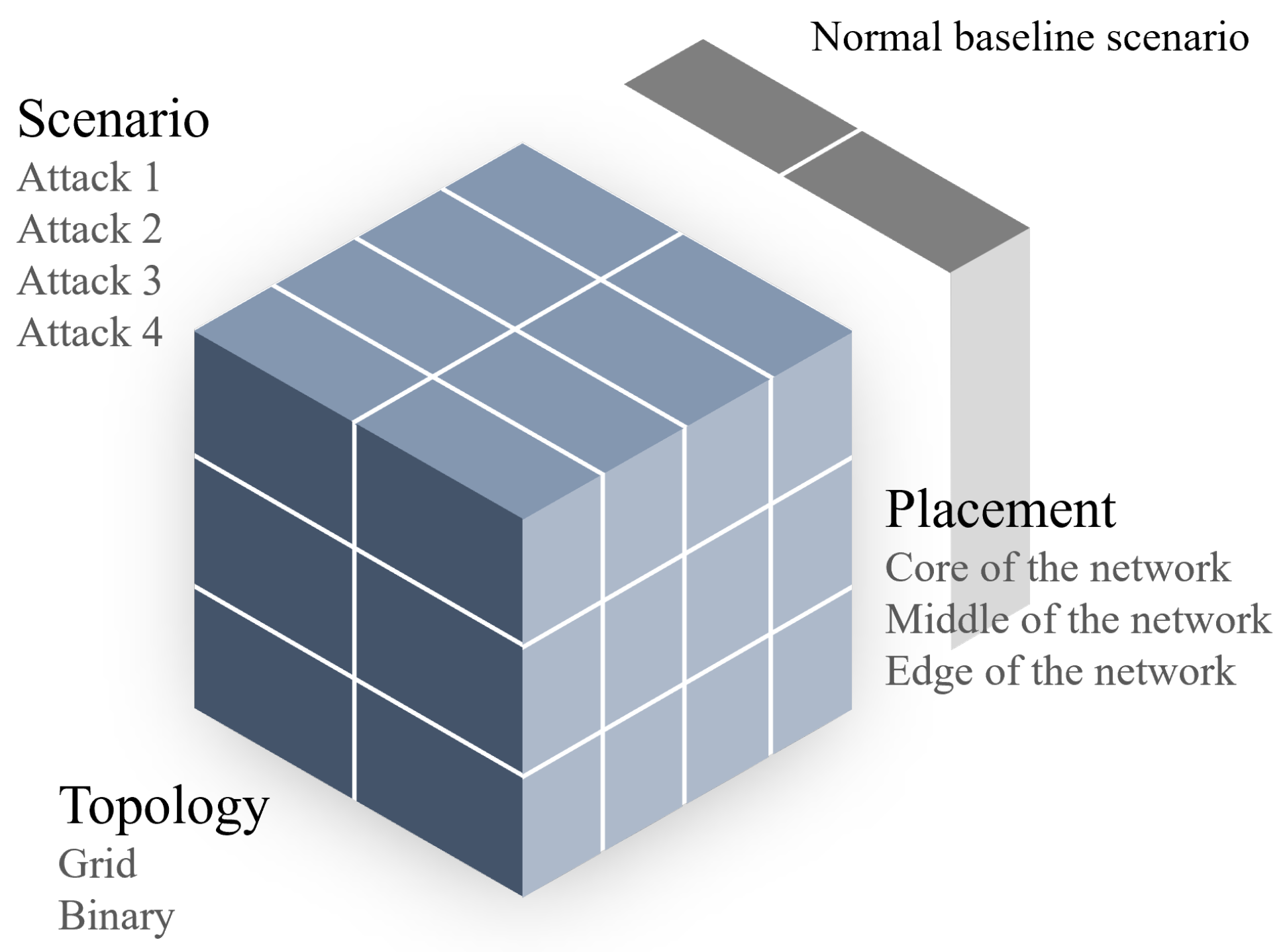
In this section, we introduce a BLC framework that enables researchers to conduct replicable experiments under predefined conditions. The framework provides a systematic approach to conducting conclusive experiments on WSNs by considering varying factors that may impact its results’ generalization. In the case of studying the impact of malicious attacks on WSNs, a researcher can leverage this framework to conduct structured experiments by considering different attack scenarios, network topologies, and attacker placements. The attack scenarios may be scaled in breadth by covering different attacks, or in depth by considering varying numbers of attackers carrying out the same attack. Figure 1 provides an illustration of the considerations of this framework. Further, we propose a set of tools that aid a researcher to conduct experiments according to this framework through the precise positioning of network nodes in the network, identifying their types, and extracting and summarizing key metrics.
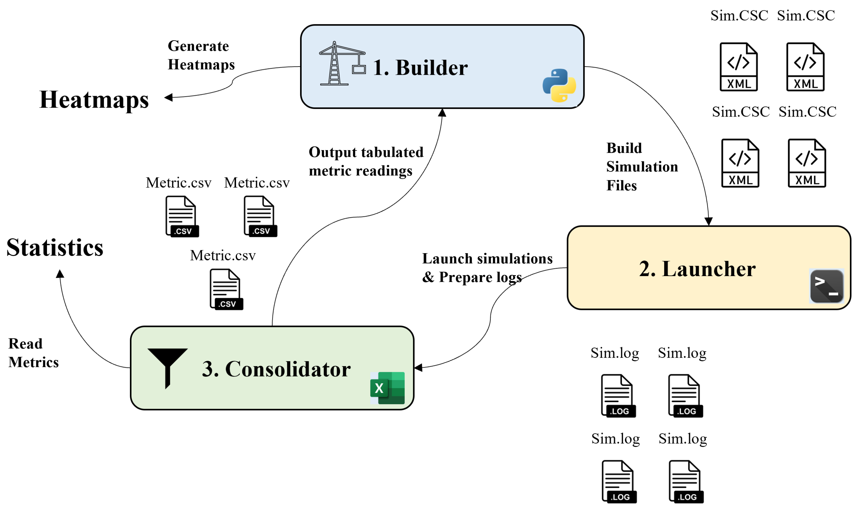
Contiki [16] provided a Java-based simulator called Cooja [15], which facilitates network debugging and performance analysis, including power tracing and profiling. However, each scenario needs to be configured manually by specifying nodes’ types and locations, run separately, and analyzed accordingly. The results collected during each simulation period provide detailed information about each node in the network. These results are often fragmented, limited, and hard to consolidate either at a holistic level or at an individual level. Analyzing both simultaneously is expected to provide further insights into how the overall network behaves during experiments. The framework offers structure and tools built upon three main components, as shown in Figure 2.
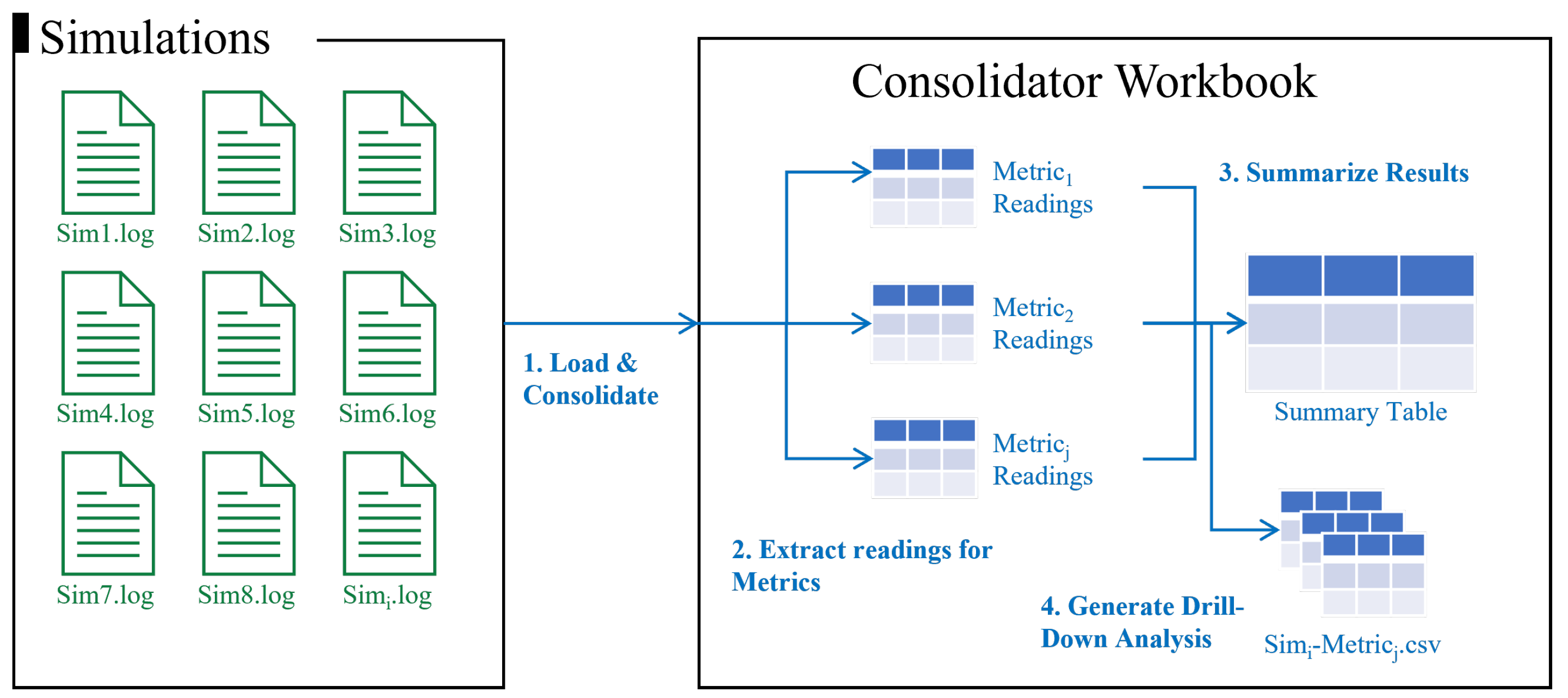
The Builder provides flexible and precise generation of Cooja automated simulation files. It can handle different classes of nodes and place each node with precision to form consistent topologies with different scenarios. The Launcher allows the running of simulation files produced by the builder in masses, with proper labeling and storing of output log files. The Consolidator consolidates all output files into one master worksheet leveraging Power Query. It analyzes and calculates the metrics and statistics of each scenario. These metrics can be interpreted through tables and charts and can also be exported to CSV files. These statistics can also be used to generate heatmaps for further analysis of the network’s state using the builder. We will discuss in detail how each component works, what are the inputs it needs, and what outputs it produces.
3.1. Builder
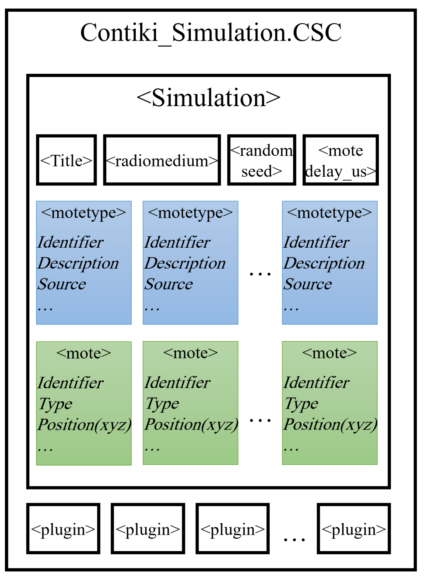
The builder facilitates the experiment setup by allowing the definition of different node/mote types and their position for the simulation to ensure the provision of customized and replicable experiments. To achieve this, the builder utilizes CSC files saved by Cooja simulation (which includes XML descriptors of the simulation environment). Each simulation file contains full configuration data, such as required Cooja extensions, simulation parameters, and information about each mote, such as type and position, as illustrated in Figure 3. In addition, the simulation file includes pointers to Contiki process source files that run for each mote type, allowing the builder to build the simulation with the correct source files for each type of node.
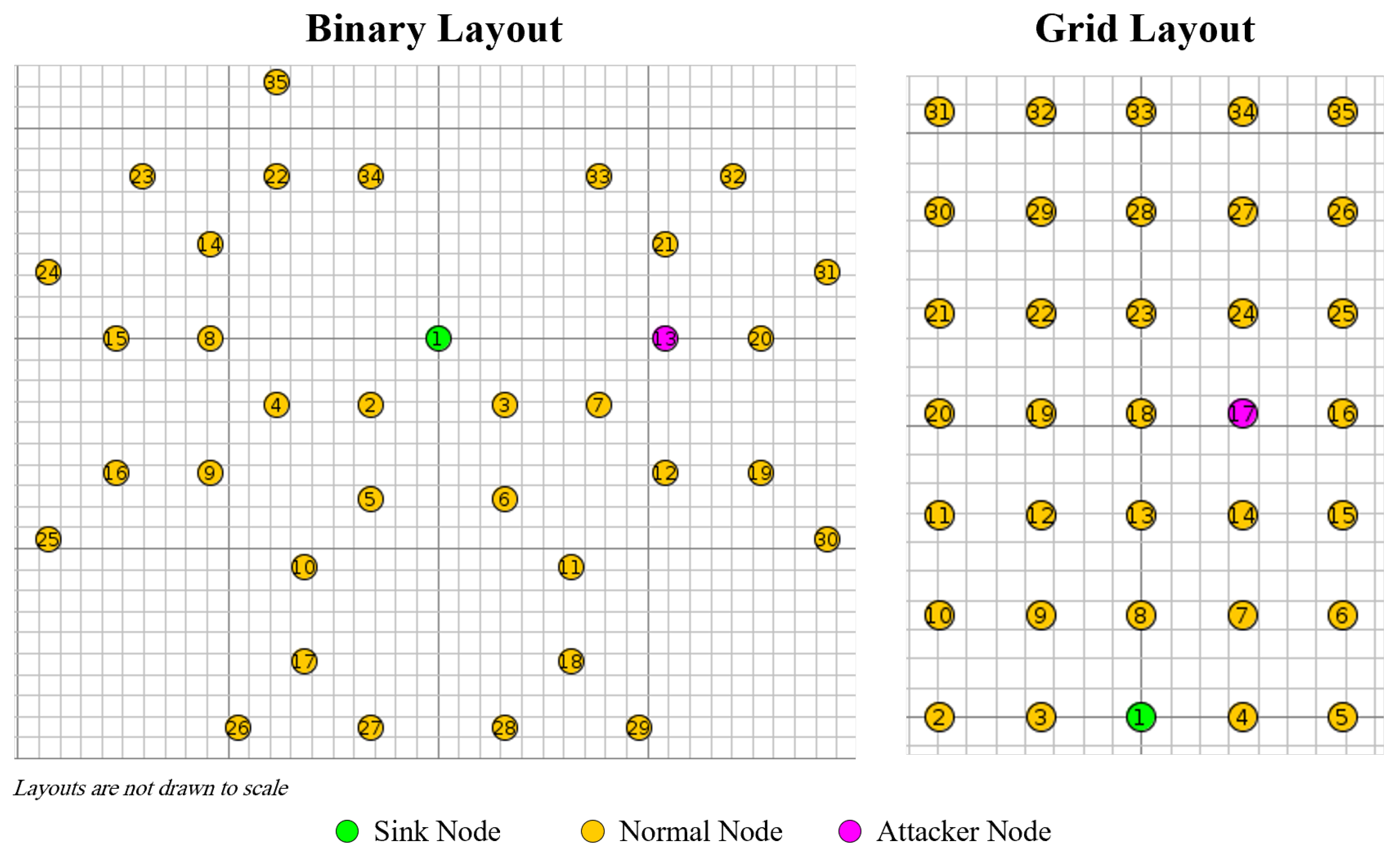
The CSC file also includes exact coordinates for each mote as it is placed in the simulation hyperplane. The builder tool can be used either to position each node programmatically or to use prebuilt methods to build two classes of layouts, which are (1) a binary layout, where each node extends the network’s coverage to a maximum of two additional nodes, and (2) a grid layout, where nodes are structured such that they are arranged in columns and rows. Both layouts are implemented by default, but the builder can still be scaled to accommodate different layouts and topologies. Both layouts offer contradicting trade-offs as the binary layouts favor covering a larger area with a finite set of devices, whereas the grid maximizes redundancy because it avails more paths to the sink for each node at the cost of the area covered. The aim is to obtain more comprehensive insights of our experiment by expanding its scope to cover two contrasting layouts that may exhibit contrasting behavior and produce different results.
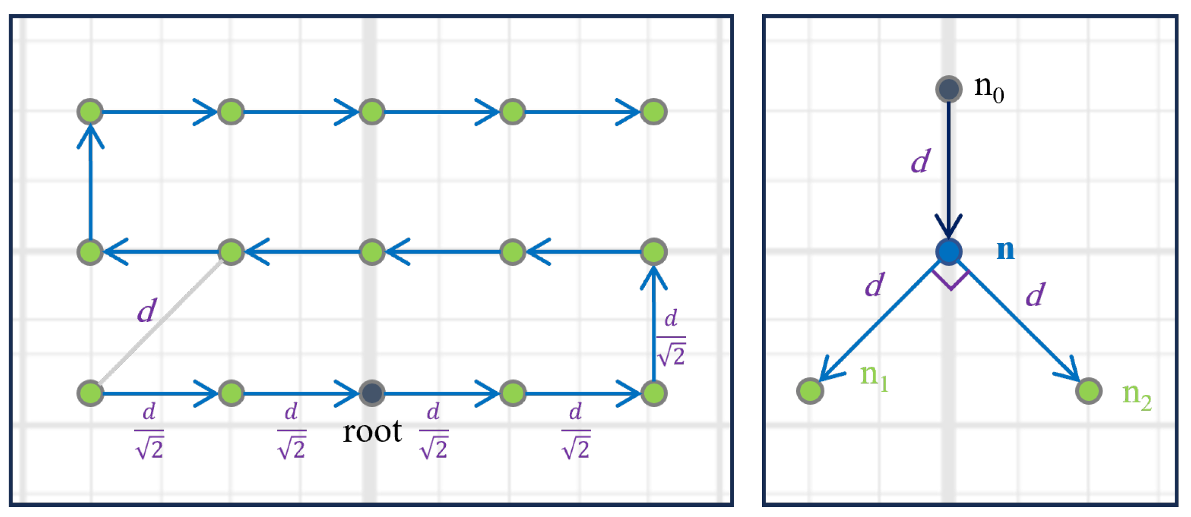
Figure 4 shows how our builder determines the coordinates of each node recursively, based on a previously generated one through the illustrative arrows. In our implementation, nodes in the binary layout are characterized by having a maximum of one potential parent. The distance between the nodes is fixed as the maximum distance for transmission range, and the angle where nodes branch is a constant 90°. The builder tool is capable of generating such networks recursively. Each node branches with two new child nodes, noting the angle of the branch vector. The coordinates for the child nodes created at each branch are calculated algebraically based on their parent’s coordinates and the angle of the parents’ branch vector. Before introducing a new node to the network, the prebuilt graph is traversed to ensure that the node to be added is not close to any other node (besides its parent) to avoid cycles and enforce the binary layout rule. If another node is found in proximity, the new node is not added, leaving its parent with only one child.
However, the grid layout is characterized by its grid-like distribution. In our approach, central nodes will have up to eight neighbors and potential parents. Our builder can have the node at the edge of the layout or position it toward the center. Provided with the number of rows and columns, the builder will build the network by generating coordinates for each node until the network is fully built. It is worth noting that the distance is shorter among vertically and horizontally adjacent nodes compared to diagonally adjacent nodes. Because the distance between a node and its diagonal neighbors is equal to d (the maximum distance), the builder uses basic trigonometry to calculate the distance between a node to its other neighbors, which is . Both layouts can be adjusted programmatically with manually specified coordinates. Further, the user may use direct access to functions for branching at specific points, allowing for more hybrid topologies to be created and merged.
Further, the user can specify which nodes run which source file. Once all parameters are specified, the user can generate the XML excerpt for the simulation parameters, which can be inserted between tags on any existing Cooja simulation file. The user can use the builder to generate as many Cooja simulation files as needed, each with its own parameters according to the experiment design. The simulation files can be run by the launcher to conduct experiments and collect datapoints for analysis. The builder can be leveraged once more to build powerful heatmaps to analyze the network’s performance in each simulation once simulations are run and data points are collected. The builder can also use performance data collected from a simulation to generate a heatmap of the network for each collected metric. This is achieved as the tool capitalizes on its prior knowledge of the positioning of nodes in the network. The heatmap serves as a powerful visual aid to spot the changes in the collected metrics.
3.2. Launcher
We also leverage a launcher to streamline the conducting of our experiments, which is a bash script used to run simulations on Cooja while labeling output logs and packet captures for future use and analysis. Once the builder generates simulation files, the launcher runs each simulation independently without loading the Cooja GUI. Thus, the launcher offloads resources on the host machine and allows experiments to run more efficiently. This feature proved to be vital for sizable simulations consisting of a large population of nodes as well as simulations where expensive processes are run (such as flooding attacks), which would overcome memory issues.
Specifically, the launcher is a bash script that interfaces with Cooja through commands. It requires the simulation name in the format “” as input. As the simulation concludes, the launcher locates the newly generated logs and properly labels and saves them with the proper name of the simulation. Both files are stored properly, ensuring they are not overwritten in the next simulation. If the simulations are run in a virtual machine, it is worth considering storing the results in a shared folder between the guest and host machines to enable faster access and allow the analysis of each scenario’s results while the next simulation is running.
3.3. Consolidator
The consolidator consolidates all output files into one master workbook leveraging Power Query. The consolidator relies on the logs generated by the simulations to calculate different metrics. This implies that the source code for the network’s nodes is programmed to output readings of desired metrics beforehand. Accordingly, log outputs include timestamps of these readings and events. Readings for each metric are collected by a specific query designed to parse for it. Readings for each metric are then stored separately for further analysis. The consolidator preprocesses all the log files resulting from simulations and records individual messages by simulation, timestamp, node ID, and output message. Each message is checked against a match of a predefined signature for each metric.
Our existing implementation collects three popular metrics for measuring the performance of the network; namely, PDR, E2E delay, and power consumption. The consolidator can be expanded to accommodate additional metrics with proper configuration. PDR is a key indicator for the quality of message transmission and reception, and by extension, the availability of the service provided by the network. E2E delay, conversely, looks at the degradation of the service resulting from delayed packets. Both measures rely on the nodes logging timestamped messages of sending and delivering data packets, which are read by the consolidator for each metric. Increased power consumption is detrimental to the lifespan of the network because it quickly depletes the nodes’ batteries. We estimated power consumption using PowerTrace [30] and the ENERGEST module. Both are used to track—at the node level during run time—how long each hardware component has been on (e.g., CPU and transmitter). If we know the rate of energy consumption for each individual component when it is used, then we can use both to calculate an estimated power consumed at a specific interval. These rates are often documented as part of the hardware specification for individual node types and can vary among different manufacturers and architectures. Table 3 illustrates the specification factors used for the Zolertia Z1 motes according to the datasheet [31]. Readings of power consumption rates are collected by reading logged messages by the nodes. The consolidator allows easy modification of these factors to scale to different hardware.
At the core of the consolidator are master lists that include all simulations and their average readings for all nodes for each metric. In addition, the consolidator includes one worksheet that includes holistic average readings for all metrics for all simulations as a summary of experiment results, as illustrated in Figure 5. The consolidator also outputs separate sheets (one for each metric) that include node-level average readings for each experiment. These can be exported to CSV files for further analysis. Because the layouts of these networks were already built using the aforementioned builder, the same tool can be fed with resulting CSV results to help generate visual heatmaps. For example, if an experiment included 6 simulations (1 for each combination of scenario–placement–topology) to collect 3 metrics, we would have 18 heatmaps, each showing average readings of each node in each simulation. This proved to be a strong analysis tool and allowed us to visually trace the impact of each attack or treatment throughout the network structure.
4. Case Study: Analyzing Flooding Attack
In this section, we will examine the impact of a flooding attack on RPL networks considering different topologies, leveraging the framework and tools proposed in Section 3.
4.1. Flooding Attack
A flooding attack is a form of DoS attack that aims to degrade or completely bring the service provided by the network to a halt. There are many forms and methods for carrying out a flooding attack that exploits weaknesses in the communication protocols stack. One such attack is a DODAG Information Solicitation (DIS) flooding attack. As per RPL specifications, the actual topology of a network is built dynamically as nodes in the network exchange information with each other. DIS messages are sent (usually as multicast) by new nodes to solicit information on available networks and candidate parents. Adjacent nodes already in the network respond by sending DIO messages to advertise their information [32]. After receiving DIO messages from neighbor nodes, the new node stops sending further solicitation messages and views all senders as prospective parents [33]. However, in a DIS flooding attack scenario, a malicious node would keep sending DIS messages excessively, overwhelming other nodes in the network and forcing them to generate additional DIO messages, which disrupts their ability to handle their roles in passing benign traffic, leading to congestion across existing links [34]. In our implementation of the attack, the malicious node is assumed to have infiltrated the network and acts as normally as other nodes until the attack is triggered. Flooding attacks are a classic example of DoS attacks. Their footprint on RPL networks has been studied widely and is shown to cause significant disruption to the networks in PDR, throughput, and power consumption [35,36]. Almomani and Alkasasbeh [37] compared flooding attacks to other DoS attacks (namely blackhole, grayhole, and scheduling attacks) and demonstrated in a simulated experiment that they cause severe damage to the target network’s lifetime and service availability.
4.2. Simulation Environment
We carried out the flooding attack in a simulated environment using Cooja and Contiki, leveraging our aforementioned framework tools to build the network and analyze our simulations. Our virtual simulation consists of two layouts (binary and grid), as discussed in Section 3, and two scenarios (one with an attacker and another without an attacker as a baseline scenario), making a total of four simulations. Each simulation consists of 35 nodes (34 sensors and one sink). Each sensor node records some observations and sends its supposed readings to the sink, which in a real application would analyze the different readings and act accordingly. The position of the attacker in central areas of each network, as illustrated in Figure 6, is neither directly adjacent to the root node nor at the edge of the network. Further details on the specifications of our setup are summarized in Table 3. After we had set up the environment, we ran all of our four scenarios using the launcher script. Afterward, we compared the performance of our network when attacked to our original baseline. This experiment aims to compare the effect of a treatment (applying flooding attack) while controlling one potential confounding variable (network topology).
4.3. Results and Analysis
The outcomes of our experiment are summarized in Table 4, where we compare the results of each attack scenario to the baseline for the respective network layout. For each metric, a darker red shading for a cell indicates a larger deviation from the most favorable reading.
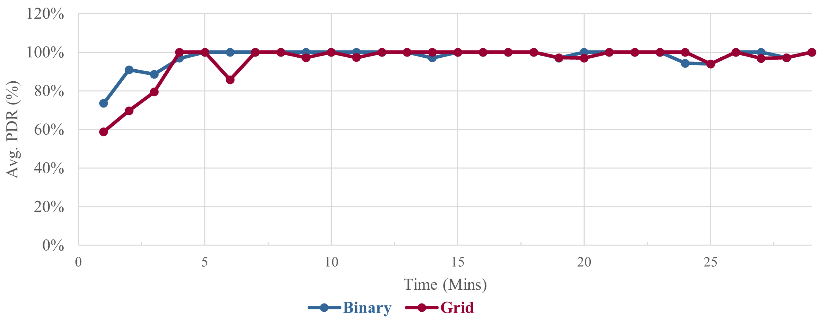
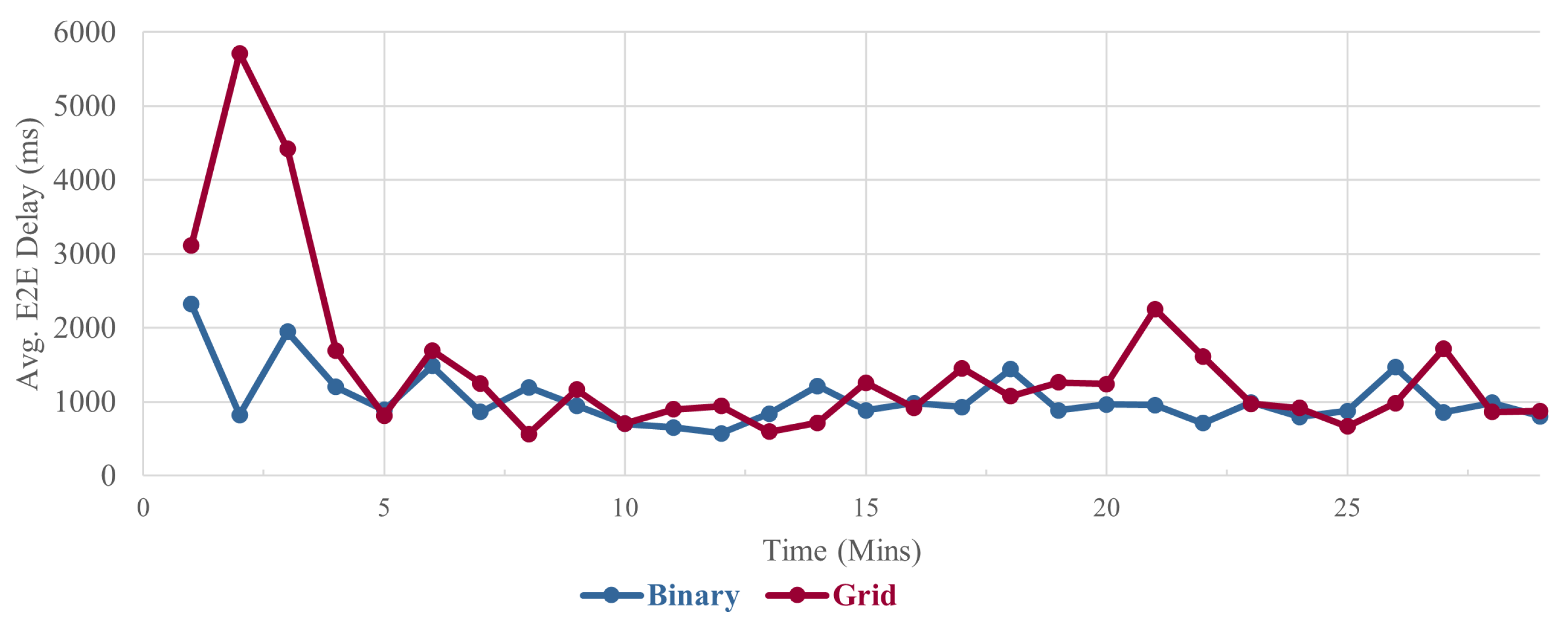
We distinguish both layouts in the baseline scenario. We note that both performed differently, with the binary topology being the most efficient across all metrics. Starting with PDR, we note that on average, it was marginally better in the binary layout compared to the grid layout. After a closer look at Figure 7, we can determine that the marginal difference is mainly driven by the extended time needed to build the grid layout and its DODAG because both layouts performed virtually the same after minute 3. For the average E2E delay, we noted significant delays in the grid layout equal to 35% more compared to the binary layout. The delays were particularly higher for the first 3 min but rapidly decreased thereafter and slightly fluctuated throughout the rest of the simulation, as visible in Figure 8. However, the grid layout still experienced more delays more often than not on average compared with the binary network.
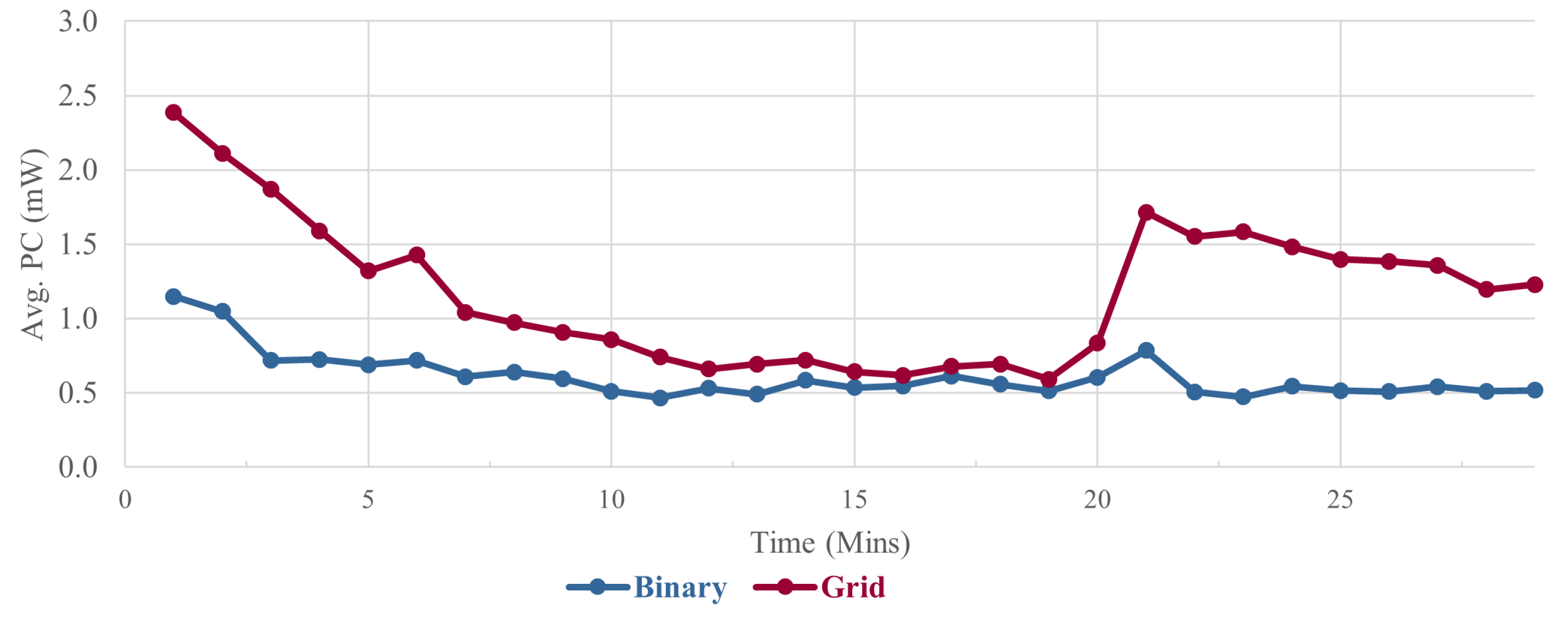
Last, we can see that the binary network showed more efficient power consumption compared to the grid layout throughout the experiment, as illustrated in Figure 9. In fact, there were periods when the power consumption for the grid layout was double and triple that for the binary (e.g., minutes 1, 6, and 21). Over the duration of the experiment, the grid layout had a 46% higher power consumption rate compared to the binary. We attribute this to the increased exchange of control messages in the grid layout because of its increased density.
The results consolidated by our consolidator (shown in Table 4) show that both layouts were impacted when exposed to flooding attacks to a varying degree. To facilitate quick analysis, particularly for larger experiments, the background color of the cells gets redder as the score gets worse for each metric. We note that the grid layout was more impacted by the attack when compared to the binary layout, implying that having more dense networks where a node has more neighbors helps the propagation of the flooding messages to a larger population of the network.
Looking at the network’s population to analyze the impact on different nodes can help us better understand the attack’s propagation and consider the severity when distributing our sensors and planning our mitigation approach. To that end, we will analyze the changes in each metric for each topology in more detail, leveraging the heatmaps generated by our framework and toolkit. There is one heatmap for each metric–topology–attack combination, where each heatmap plots all nodes as colored circles in their corresponding coordinates and highlights potential links as lines. The sink node is colored in light green, whereas the attacker node is highlighted in pink. Other nodes are labeled with their node number as well as the change in the analyzed metric compared to the normal baseline. The nodes themselves are also colored based on the severity of that change for easier interpretation. If there is no change, the node is transparent. As the change becomes more significant, the more saturated the color of the node becomes. If the change reflects an improvement, the color changes to green. If the change reflects a deterioration, the color changes toward red. Thresholds for the significance and polarity of interpreting these changes are defined for each metric and can be customized. If there are no readings for that specific node, the node is labeled with “No data” and colored in gray.
4.3.1. Impact on Packet Delivery Ratio
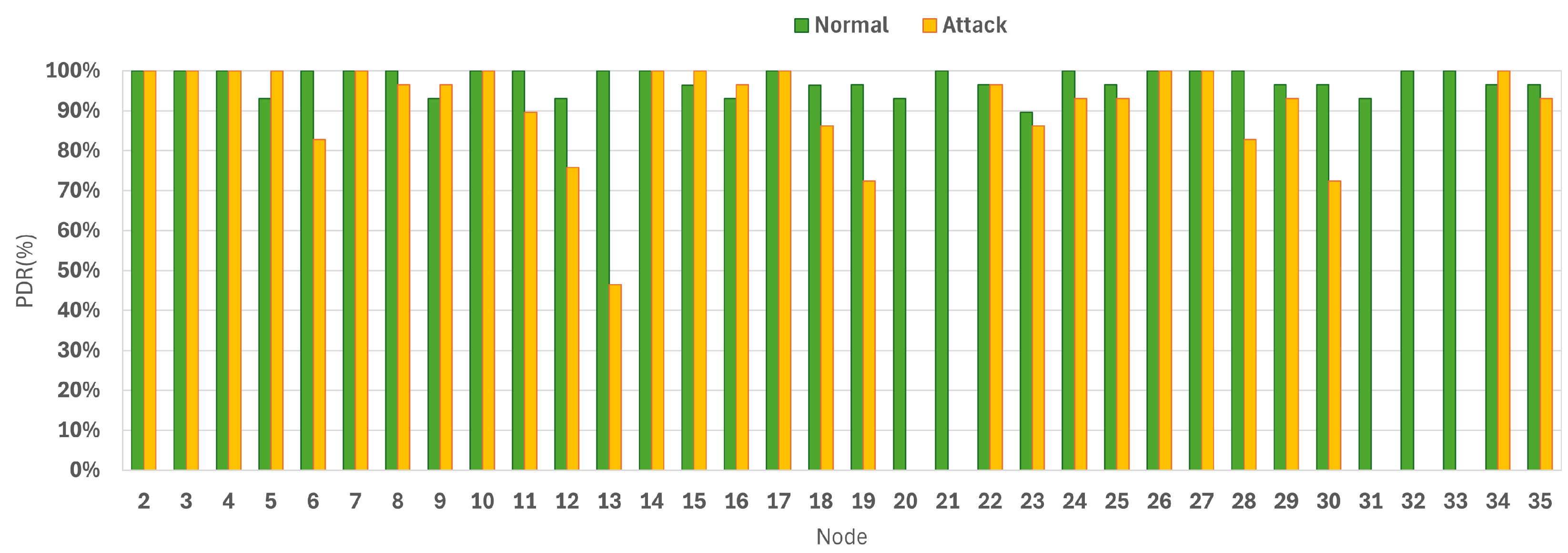
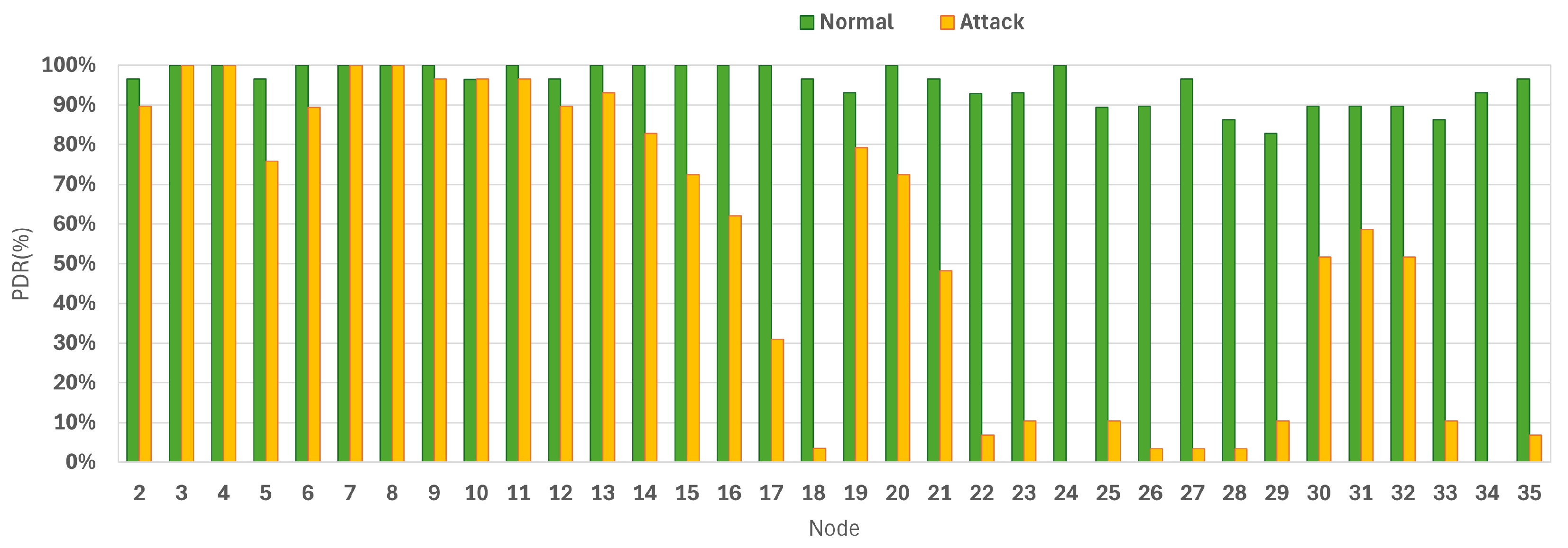
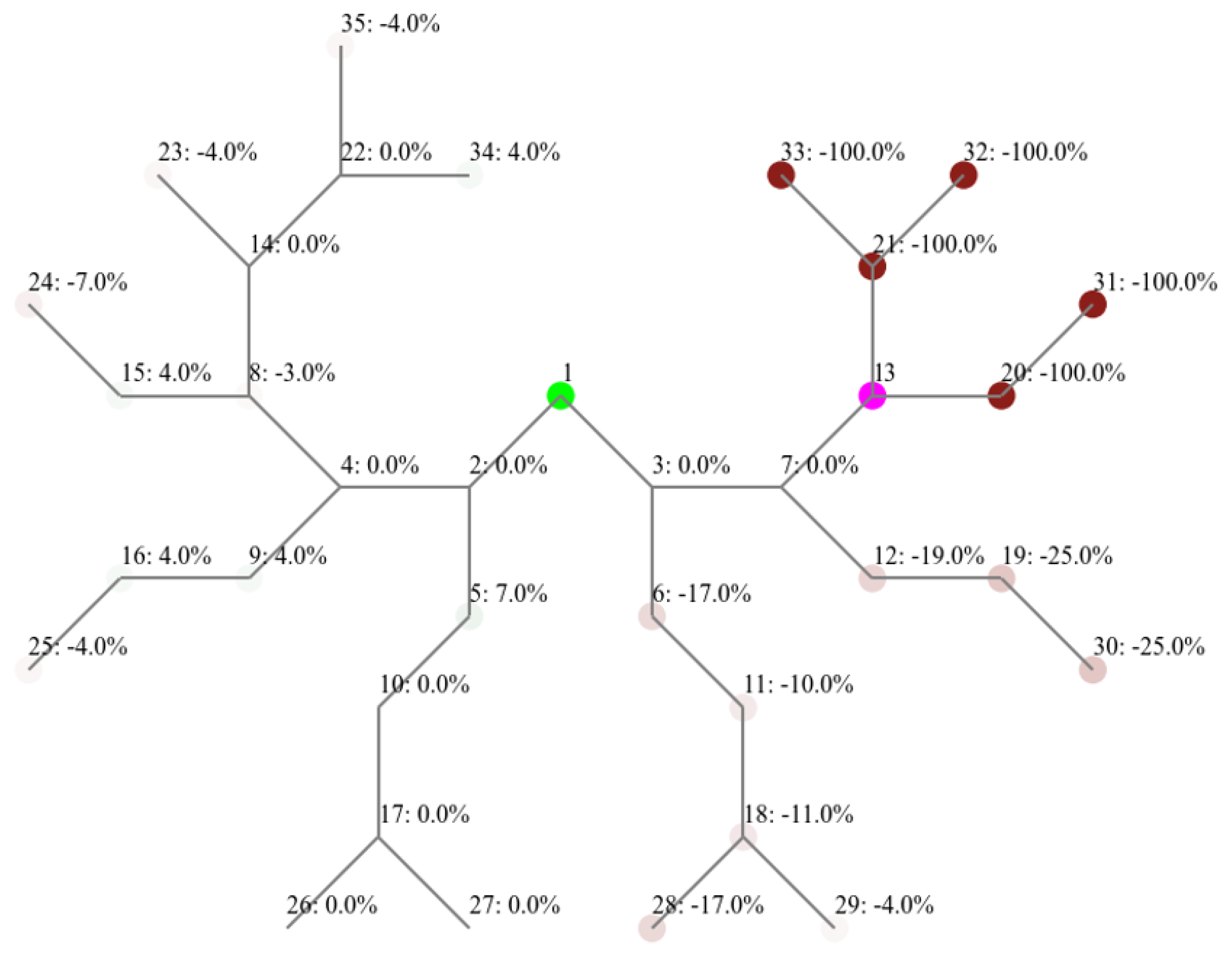
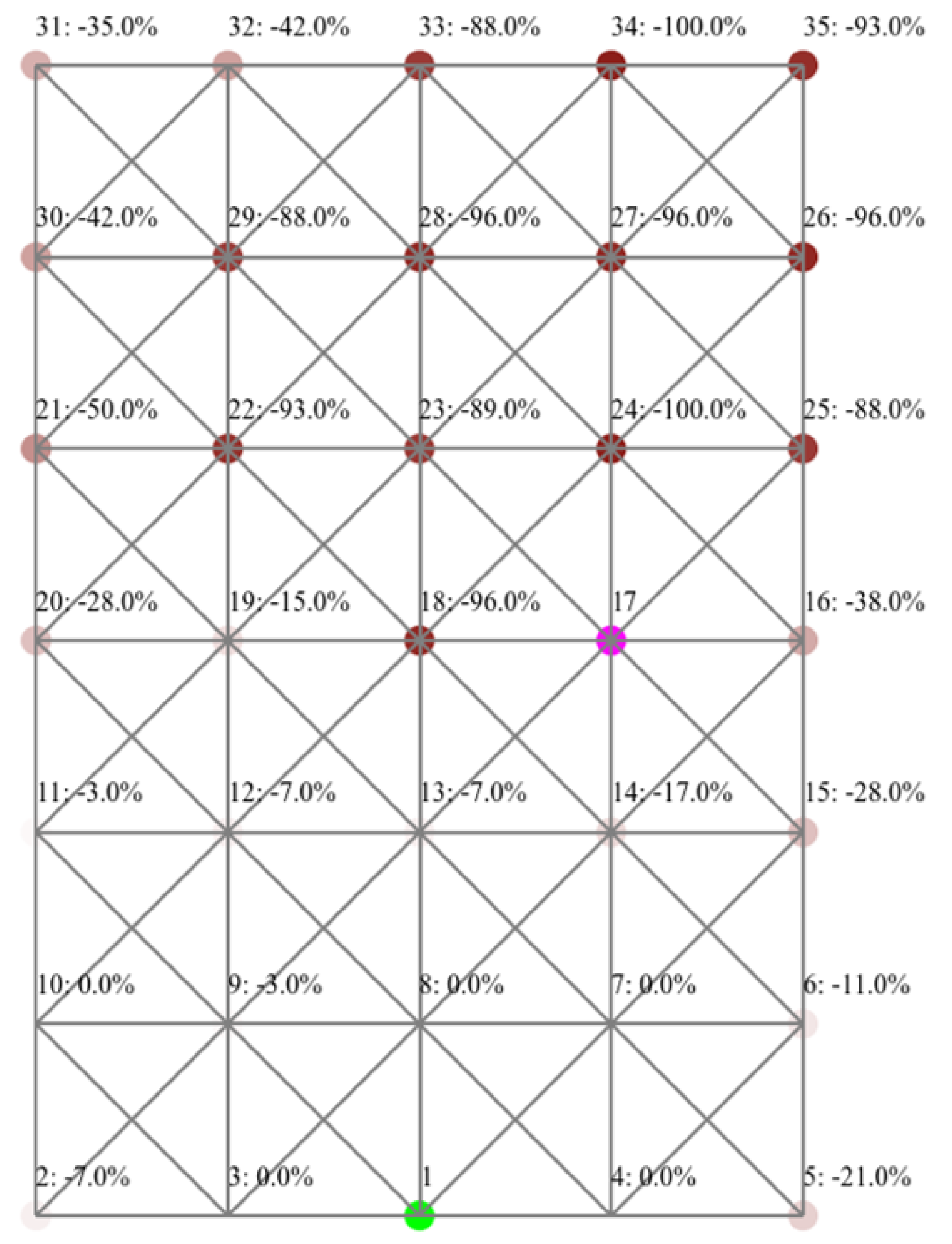
Table 4 shows that the PDR for the binary layout network decreased by 19% under the flooding attack, compared to a 44% decrease in the grid layout. Moreover, Figure 10 and Figure 11 illustrate the average PDR for each node of the binary and grid layouts, comparing the attack’s impact with the normal baseline. In a regular scenario, most of the nodes in both layouts achieve a PDR score of 100%. The binary layout exhibits a minimum PDR of 90%, as shown in Figure 10, whereas the grid layout shows a minimum PDR of 83%, as illustrated in Figure 11. On the other hand, under the flooding attack, multiple nodes in both layouts failed to deliver any data packets and scored 0% PDR. We utilized the heatmaps generated by our tools to analyze how individual nodes performed during each simulation, which gives us insights into how the attack propagates. Figure 12 shows a heatmap for the changes in the PDR across the binary network nodes after the attack compared to the normal baseline scenario (without the attack). Figure 13 shows the same comparison for the grid layout network.
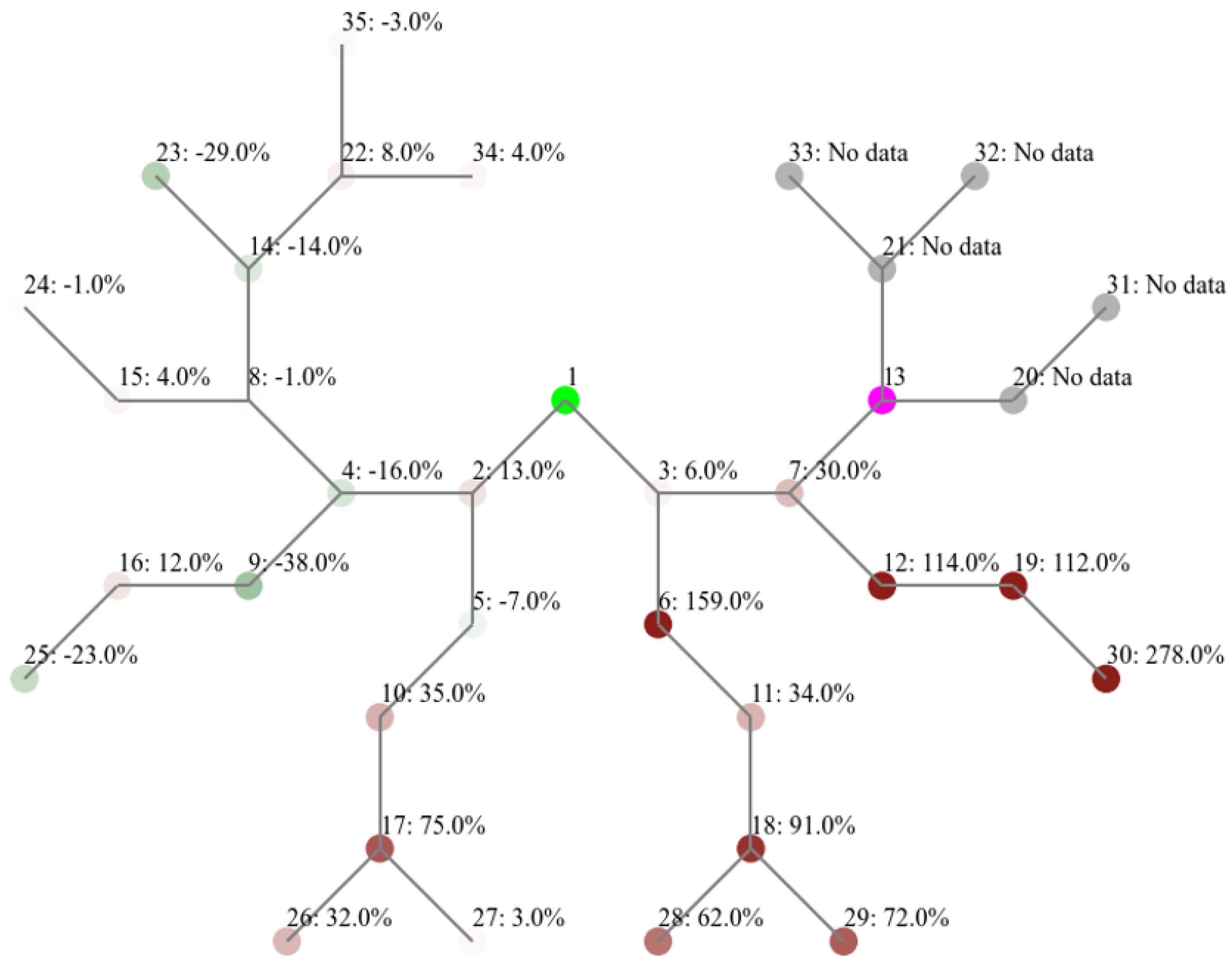
Starting with the binary layout, Figure 12 demonstrates that the child nodes of the attacker failed to deliver any messages to the sink. The attacker’s parent, however, was not impacted, but the average PDR of its other branch (nodes 12, 19, and 30) was notably decreased by 23% on average. The same can also be noted—to a lesser degree—for the further outer branch (nodes 6, 11, 18, 28, 29), which showed a decrease in PDR by an average of 11.8%. The other half of the binary layout showed no significant changes.
As for the grid layout, as Figure 13 reveals, we can see that 13 out of 33 benign nodes (excluding the sink and the attacker) had a decrease in PDR by 50% or more. The most impacted nodes are those closer to the attacker and further away from the sink. We notice that nodes adjacent to the attacker but closer to the sink (nodes 13, 14, and 15) are significantly less impacted compared to those that are further from the sink (nodes 24, 23, 25). Apparently, node 18 changed its parent as the experiment progressed and lost all subsequent packets. The effect of the attack in this layout propagated to a larger and further population compared to the binary layout. For example, it reached node 5, which is one hop away from the sink and two hops away from the attacker.
4.3.2. Impact on End-to-End Delay
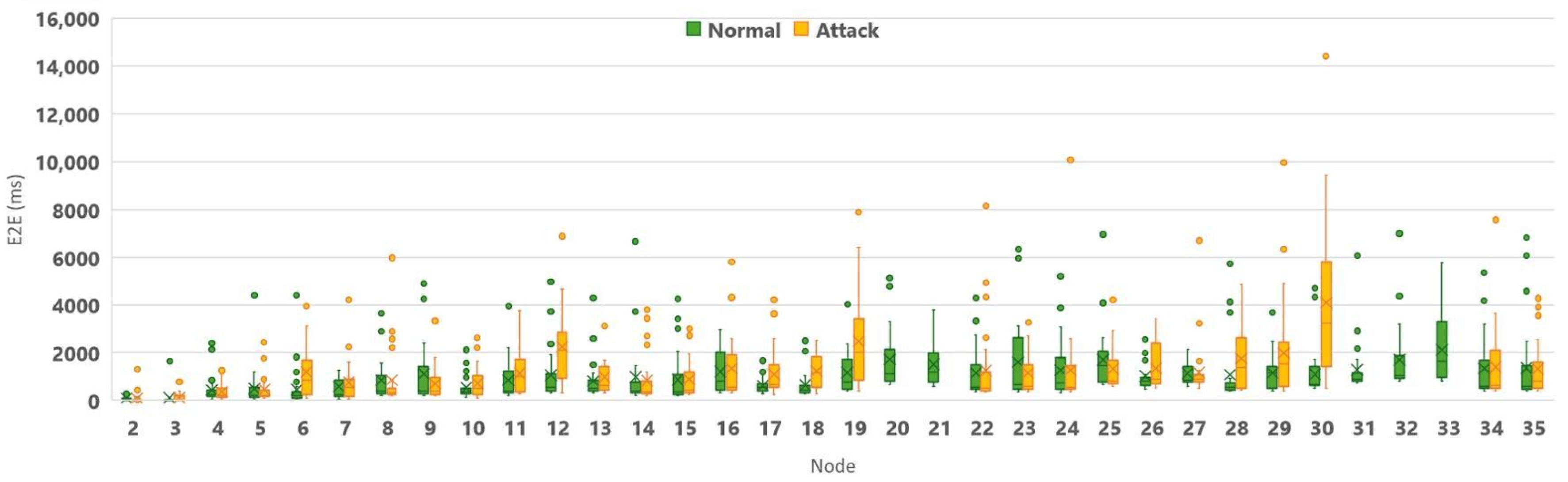
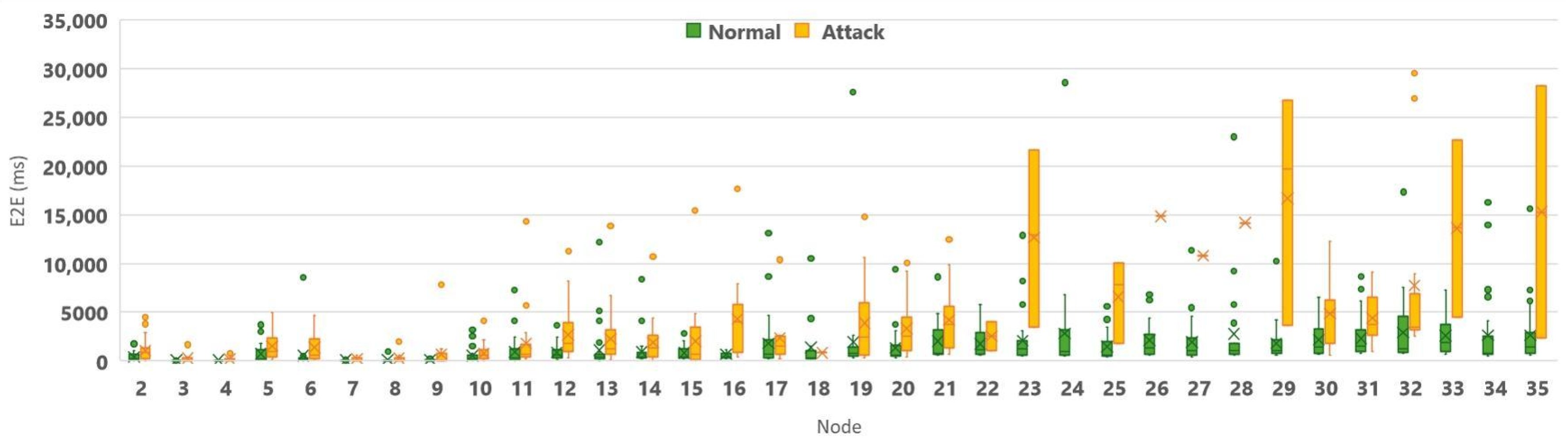
The average E2E delay for binary layout networks, as demonstrated in Table 4, following the flooding attack increased by 15% compared to the normal scenario, unlike the grid layout, where delays in message delivery increased by 72%. Figure 14 and Figure 15 provide boxplots that detail statistics for E2E readings for all messages sent by each node of the binary and grid layouts, under the normal and attack scenarios. Each data point represents the E2E delay of one delivered message throughout each simulation. For each node, scenario pair, we plotted a box representing the interquartile range (bounded by Q1 and Q3), a line indicating the median, a cross indicating the arithmetic mean, and whiskers extending the minimum and maximum values (excluding outliers, which were plotted as individual dots). These figures aim to compare the impact of the attack with the normal baseline. Irrespective of the attack, the minimum delay the nodes recorded in both layouts was 27 milliseconds. However, the maximum delay observed in a normal scenario for the binary layout was approximately 7 s, in contrast to the roughly 14 s delay logged under attack, as depicted in Figure 14. Nodes 20, 21, 31, 32, and 33 had no messages delivered when their parent (node 13) was carrying the attack. Accordingly, Figure 14 does not plot any readings. As for the grid layout, its maximum delay reached up to 28 s in normal network operations and 30 s when the network was under attack, which is illustrated in Figure 15. Nodes 26, 27, and 28 in the attack scenario for the grid layout had a single message delivered, and thus, the mean and median are plotted using the same value. A closer look provides further insights into how each network behaved under the attack, as illustrated in Figure 16 and Figure 17 for the binary and grid layouts, respectively.
Because the child nodes of the attacker in the binary layout had a PDR of 0%, there were no messages to be delivered and, consequentially, no delay to be measured as presented in Figure 16. Although the attacker’s parent witnessed 30% additional delays, its other branch (consisting of nodes 12, 19, and 30) were the most impacted. Across the network, node 30 recorded the largest average delay of 4101 ms ms, followed by node 19 with a delay of 2477 ms, which corresponds to an increase of 278% and 119%, respectively, from their baseline levels. It is noted that the impact of E2E delays spilled over to other branches and impacted a larger proportion of the network. Furthermore, some nodes in further branches recorded notable improvements (e.g., nodes 9, 23, 25, and 4), which slightly offset the average delay of the overall network. It is observed that these nodes are on the other branch away from the attacker. This emphasizes the role of the heatmap in helping us break down the impact on the network and obtain insights that would not have been visible if we measured the performance as an overall.
As for the grid layout, shown in Figure 17, we notice an increased spread of impacted nodes across the network, demonstrating the ripple effect of the flooding attack. Twenty-six nodes witnessed increased delays by more than 100% as a result of the attack. Almost all nodes suffered extensive delays, including some nodes that are close to the sink. For example, node 3 is adjacent to the sink and recorded a 422% increase in delays. Although the attacker’s direct neighbors were significantly impacted, node 18 showed a 40% improvement in E2E delay. After further examination, this was shown to be a measurement of the only packet that was delivered according to the PDR heatmap (4% PDR in Figure 13).
4.3.3. Impact on Power Consumption
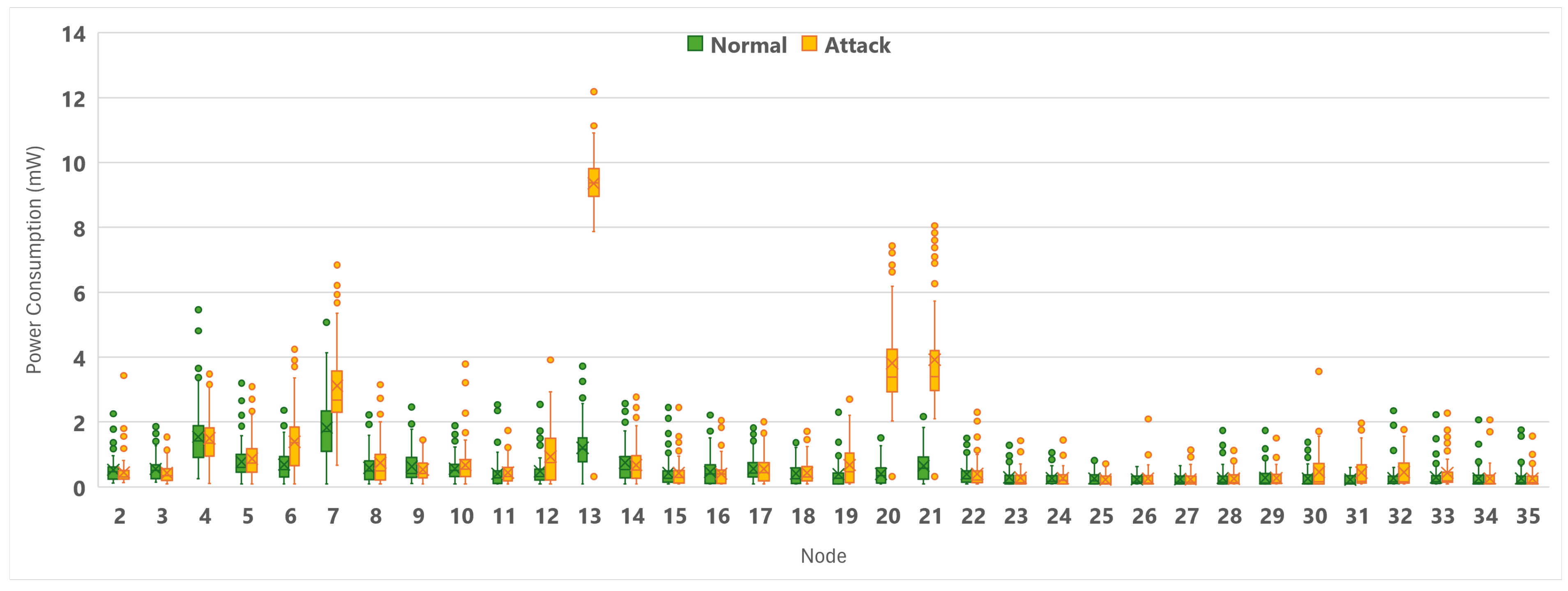
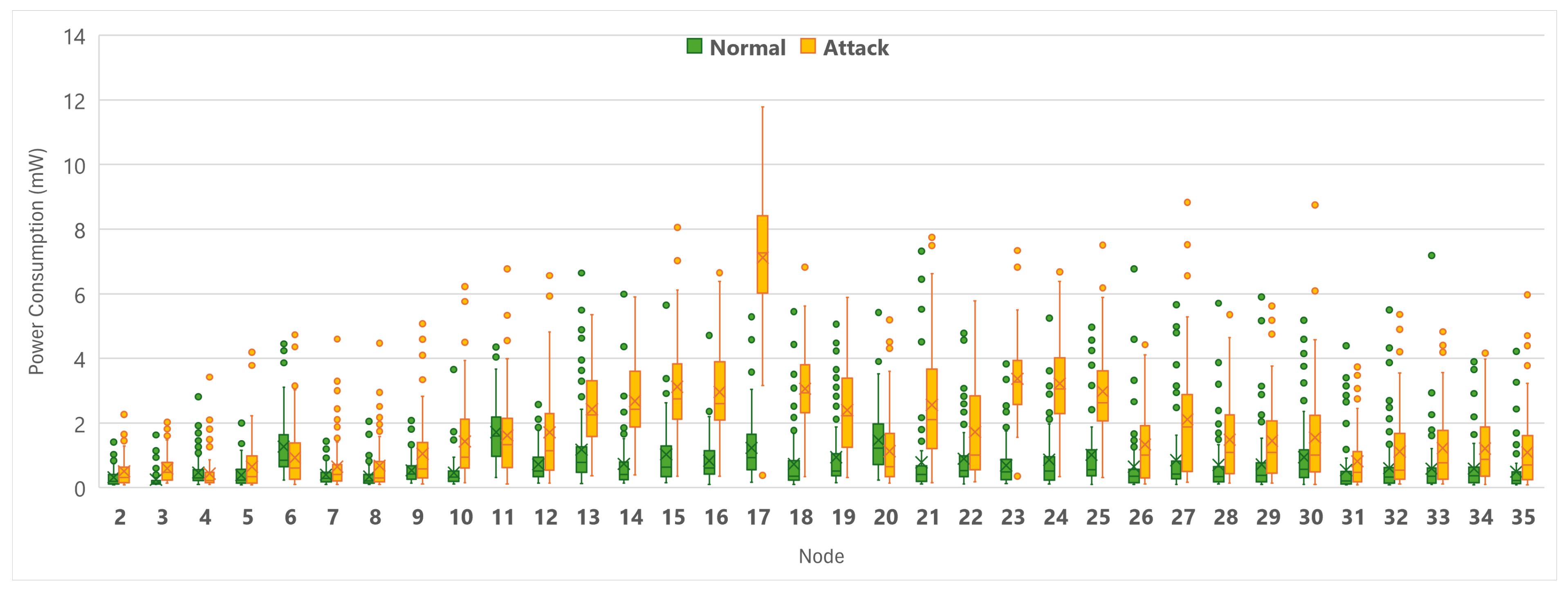
The flooding attack increased the power consumption in binary networks by 55% as presented in Table 4. At the same time, the same metric for the grid layout increased by 120%. The boxplots in Figure 18 and Figure 19 present detailed statistics for the power consumption of each node in both layouts (binary and grid, respectively). Each data point represents one 20-s reading of power consumption by the node. A total of 90 readings were collected for each node throughout each simulation. These boxplots compare the impact of the attack with the normal baseline. The minimum power consumption for both layouts was around 0.09 mW, and this was seen in both normal and attack scenarios. However, the maximum consumption increased from about 5.5 mW in the normal scenario to 12.5 mW under flooding attacks, presented in Figure 18. For the grid layout, the maximum consumption increased from about 7.3 mW in the normal scenario to 11.8 mW under flooding attacks, shown in Figure 19. A drill-down into the performance of individual nodes is summarized in Figure 20 for the binary layout, and Figure 21 for the grid layout.
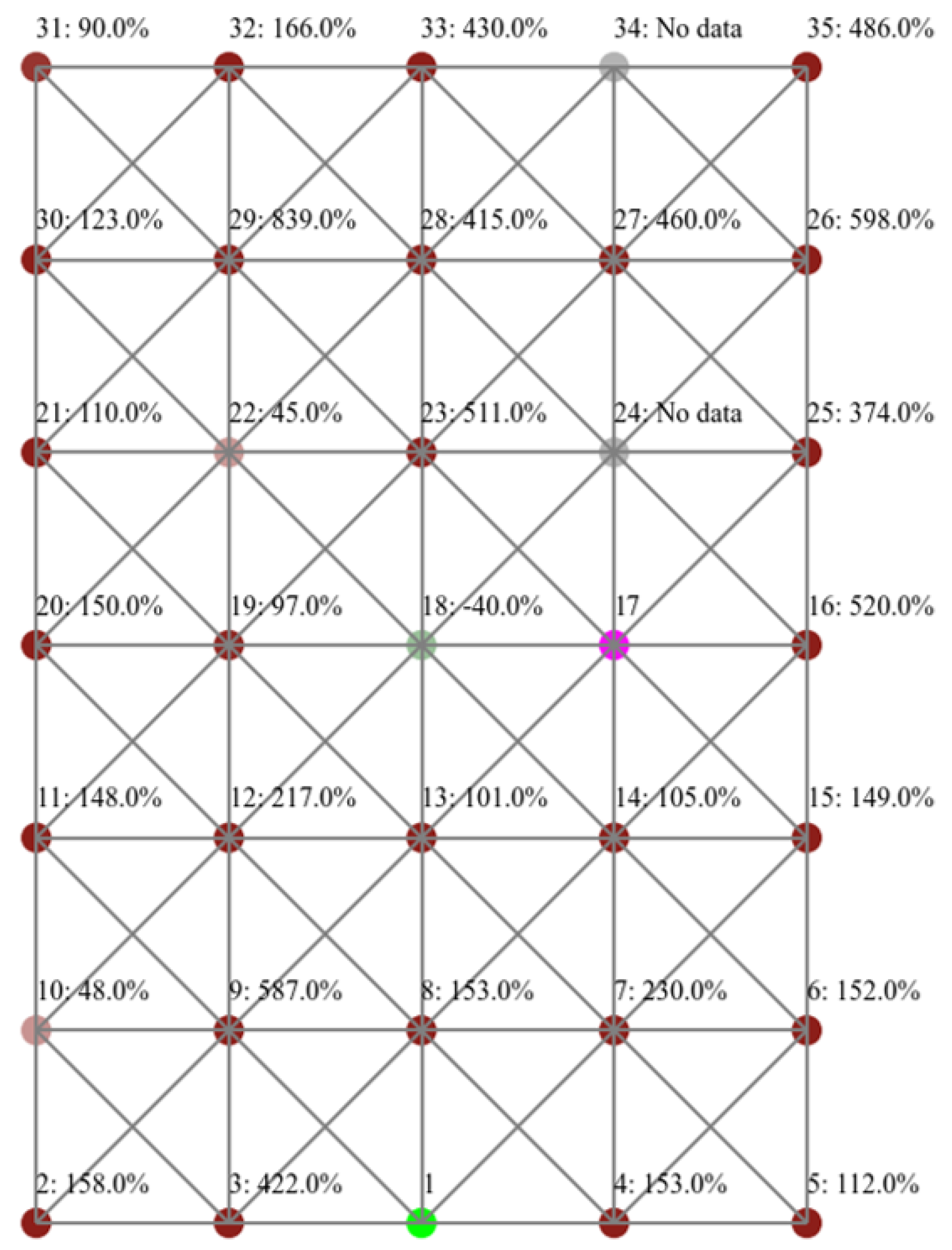
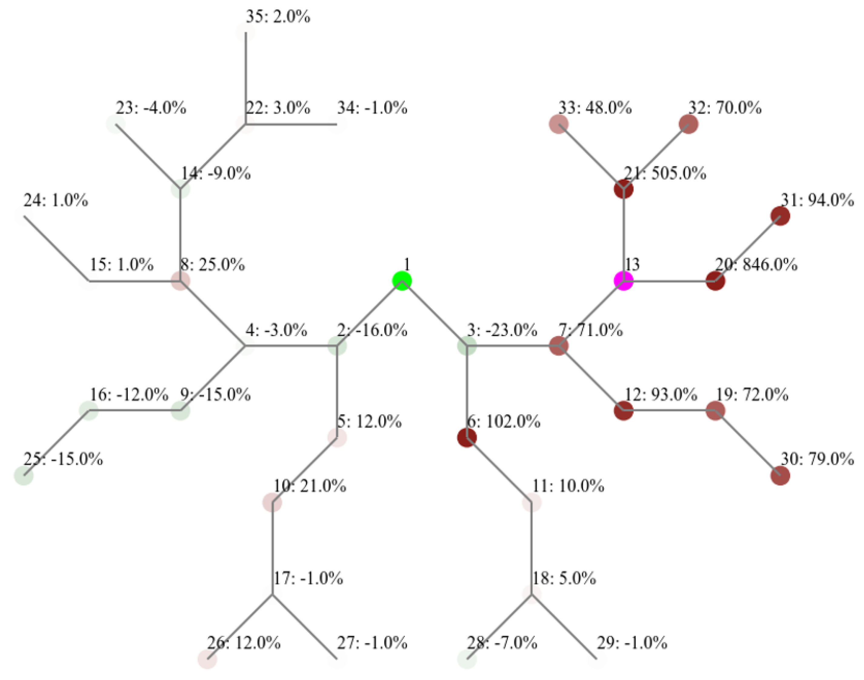
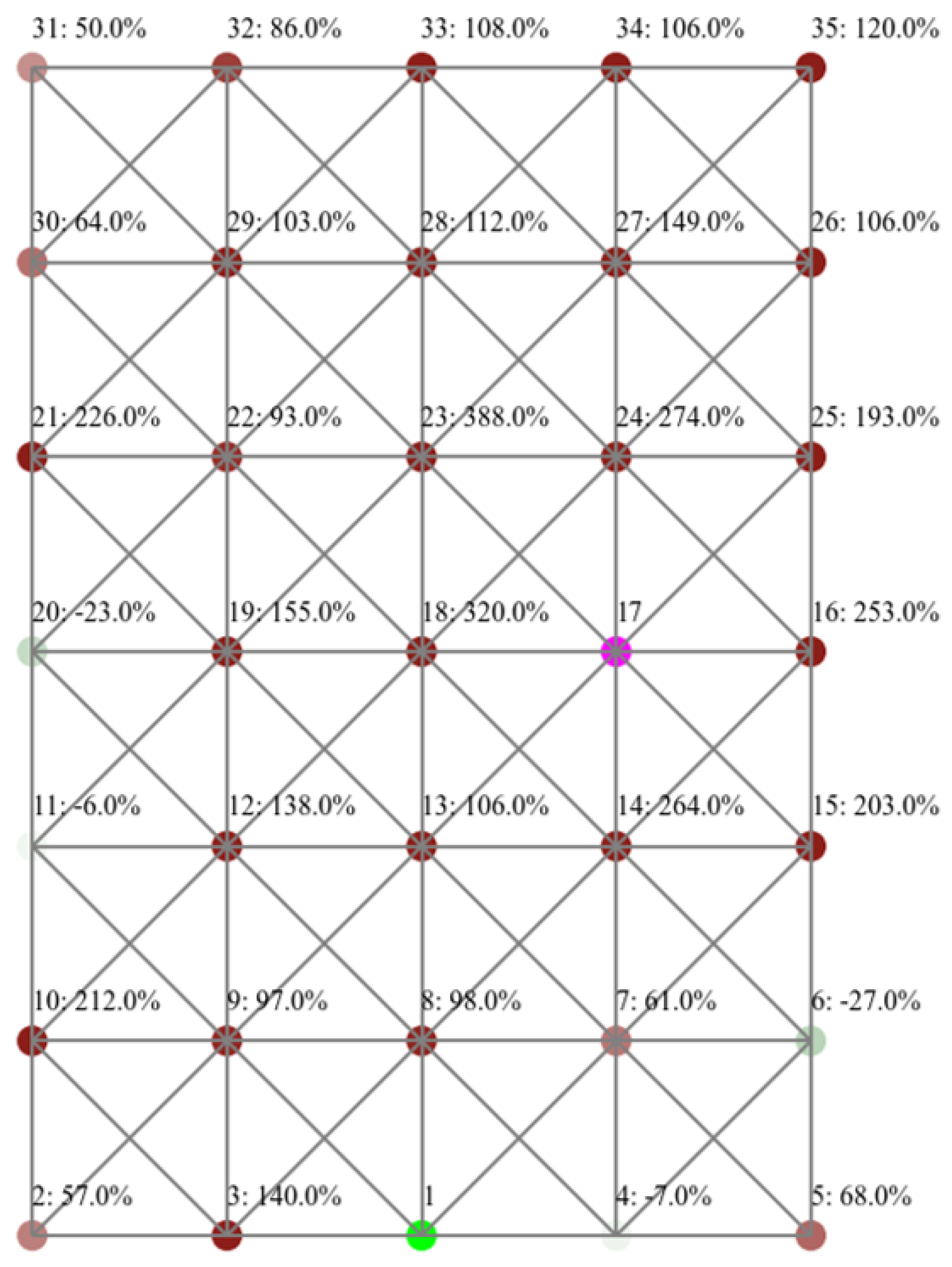
Although both binary and grid layouts were impacted to varying degrees, we notice a common pattern in both layouts: the nodes closer to the attacker are more affected by the attack and thus have a shorter lifetime. In the case of the binary layout, the child nodes of the attacker (nodes 20 and 21) had the most increase in terms of power consumption (by 846% and 505%, respectively). Similarly for the grid layout, adjacent nodes to the attacker showed the highest increase in power consumption across the network. This can be seen through nodes 23, 18, and 24, which increased by 388%, 320%, and 274%, respectively.
Additionally, we also notice that some nodes further away from the attacker showed a slight decrease in power consumption. This is applicable to both the binary layout (e.g., nodes 2 and 3), and the grid layout (e.g., nodes 6 and 23). However, one major distinction between the two layouts is that the effect of power consumption was more contained in the binary layout compared to that of the grid layout. In the binary layout, Figure 20 points out that the average power consumption for the nodes in the right-hand branch where the attacker is located increased by 130%, whereas that of the left-hand branch away from the attacker did not show visible changes. The same cannot be said for the grid layout, Figure 21, because some nodes closer to the sink and further from the attacker demonstrated a significant increase in power consumption, such as node 10, which showed an increase by 212%. The lifespan of the sink and its surrounding nodes is critical for the lifetime of the overall network because it serves the only link for further nodes to get their messages transmitted. Accordingly, we believe that a flooding attack would have a devastating impact if the attacker is positioned closer to the sink.
5. Conclusions and Future Works
In this paper, we presented a structured framework for conducting replicable simulations to study WSNs. It calls for the consideration of different factors when assessing the network performance, such as different nodes’ distribution, source codes (including attack scenarios), and node placements. The framework is complemented with tools that help with conducting experiments by considering different stages, from building each simulation to carrying out the experiments until consolidating the results and analyzing its outcomes. We demonstrated the adoption of such a framework when studying the impact of flooding attacks on two contrasting network topologies (grid and binary). The results showed that the flooding attack had a lesser effect on the binary layout network than the grid layout. After the attack, the PDR decreased by 19% for the binary layout and 44% for the grid layout. End-to-end delay increased by 15% for the binary layout and 72% for the grid layout. Additionally, power consumption increased by 55% for binary networks and 120% for the grid layout. These outcomes emphasize the need to consider network layouts since different topologies showed varying impacts. As a future work, we intend to scale our tools to consider further network topologies (such as Linear, Ring, and Random). Further, we aim to embed applicable capabilities of our tools to interface directly with Cooja for easier and faster conduction of experiments by building on the architecture of ViTool [27], which is modular, scalable, and interfaced with Cooja stack. Further, our study of a flooding attack has demonstrated the attack’s detrimental impact on the performance of the overall network. We also noted that individual nodes were impacted differently to varying degrees, with some nodes recording improvements in their average readings. Accordingly, we believe the framework and tools proposed offer an opportunity for a new approach to analyzing the impact of attacks, which focuses on the behavior of individual nodes.
Author Contributions
Conceptualization, R.A. and F.A.; Methodology, R.A., H.A. and F.A.; Software, R.A.; Validation, R.A., H.A. and F.A.; Formal Analysis, R.A., H.A. and F.A.; Investigation, R.A.; Resources, R.A.; Data Curation, R.A.; Writing—Original Draft Preparation, R.A., H.A. and F.A.; Writing—Review & Editing, H.A., F.A.; Visualization, R.A.; Supervision, F.A. All authors have read and agreed to the published version of the manuscript.
Funding
This research received no external funding.
Data Availability Statement
The raw data supporting the conclusions of this article will be made available by the authors on request.
Conflicts of Interest
Author Rakan Alghofaili were employed by the company Technical Services, Saudi Aramco. The remaining authors declare that the research was conducted in the absence of any commercial or financial relationships that could be construed as a potential conflict of interest.
References
- Lata, S.; Mehfuz, S.; Urooj, S. Secure and Reliable WSN for Internet of Things: Challenges and Enabling Technologies. IEEE Access 2021, 9, 161103–161128. [Google Scholar] [CrossRef]
- Muzammal, S.M.; Murugesan, R.K.; Jhanjhi, N.Z. A Comprehensive Review on Secure Routing in Internet of Things: Mitigation Methods and Trust-based Approaches. IEEE Internet Things J. 2020, 4662, 4186–4210. [Google Scholar] [CrossRef]
- Swessi, D.; Idoudi, H. A Survey on Internet-of-Things Security: Threats and Emerging Countermeasures. Wirel. Pers. Comm. 2022, 124, 1557–1592. [Google Scholar] [CrossRef]
- Saravanan, G.; Parkhe, S.S.; Thakar, C.M.; Kulkarni, V.V.; Mishra, H.G.; Gulothungan, G. Implementation of IoT in production and manufacturing: An Industry 4.0 approach. Mater. Today Proc. 2022, 51, 2427–2430. [Google Scholar] [CrossRef]
- Azzedin, F.; Suwad, H.; Alyafeai, Z. Countermeasureing zero day attacks: Asset-based approach. In Proceedings of the 2017 International Conference on High Performance Computing & Simulation (HPCS), Genoa, Italy, 17–21 July 2017; pp. 854–857. [Google Scholar]
- Suwad, H.I.M.; Azzedin, F.A.M. Asset-Based Security Systems and Methods. U.S. Patent 11,347,843, 31 May 2022. [Google Scholar]
- Azzedin, F.; Suwad, H.; Rahman, M.M. An Asset-Based Approach to Mitigate Zero-Day Ransomware Attacks. Comput. Mater. Contin. 2022, 73, 3003–3020. [Google Scholar] [CrossRef]
- Azzedin, F.; Albinali, H. Security in internet of things: Rpl attacks taxonomy. In Proceedings of the 5th International Conference on Future Networks & Distributed Systems, Dubai, United Arab Emirates, 15–16 December 2021; pp. 820–825. [Google Scholar]
- Le, A.; Loo, J.; Lasebae, A.; Vinel, A.; Chen, Y.; Chai, M. The impact of rank attack on network topology of routing protocol for low-power and lossy networks. IEEE Sens. J. 2013, 13, 3685–3692. [Google Scholar] [CrossRef]
- Panda, N.; Supriya, M. Blackhole Attack Impact Analysis on Low Power Lossy Networks. In Proceedings of the 2022 IEEE 3rd Global Conference for Advancement in Technology (GCAT), Bangalore, India, 7–9 October 2022; pp. 1–5. [Google Scholar] [CrossRef]
- Tripathi, M.; Gaur, M.S.; Laxmi, V. Comparing the impact of black hole and gray hole attack on LEACH in WSN. Procedia Comput. Sci. 2013, 19, 1101–1107. [Google Scholar] [CrossRef]
- Iqbal, M.M.; Ahmed, A.; Khadam, U. Sinkhole Attack in Multi-sink Paradigm: Detection and Performance Evaluation in RPL based IoT. In Proceedings of the 2020 International Conference on Computing and Information Technology (ICCIT-1441), Tabuk, Saudi Arabia, 9–10 September 2020; pp. 1–5. [Google Scholar] [CrossRef]
- Sun, X.; Wang, G.; Xu, L.; Yuan, H. Data replication techniques in the Internet of Things: A systematic literature review. Libr. Hi Tech 2021, 39, 1121–1136. [Google Scholar] [CrossRef]
- Argota Sánchez-Vaquerizo, J. Getting real: The challenge of building and validating a large-scale digital twin of Barcelona’s traffic with empirical data. ISPRS Int. J. Geo-Inf. 2022, 11, 24. [Google Scholar] [CrossRef]
- Osterlind, F.; Dunkels, A.; Eriksson, J.; Finne, N.; Voigt, T. Cross-Level Sensor Network Simulation with COOJA. In Proceedings of the 2006 31st IEEE Conference on Local Computer Networks, Tampa, FL, USA, 14–16 November 2006; pp. 641–648. [Google Scholar] [CrossRef]
- Oikonomou, G.; Duquennoy, S.; Elsts, A.; Eriksson, J.; Tanaka, Y.; Tsiftes, N. The Contiki-NG open source operating system for next generation IoT devices. SoftwareX 2022, 18, 101089. [Google Scholar] [CrossRef]
- Alghofaili, R.I. Impact and ML-Based Detection of Denial-of-Service Attacks on Wireless Sensor Networks. Master’s Thesis, King Fahd University of Petroleum and Minerals, Dhahran, Saudi Arabia, 2023. [Google Scholar]
- Ramya, P.; Sairamvamsi, T. Impact Analysis of Blackhole, Flooding, and Grayhole Attacks and Security Enhancements in Mobile Ad Hoc Networks Using SHA3 Algorithm. In Lecture Notes in Electrical Engineering; Springer: Singapore, 2018; pp. 639–647. [Google Scholar] [CrossRef]
- Mayzaud, A.; Badonnel, R.; Chrisment, I. A distributed monitoring strategy for detecting version number attacks in RPL-based networks. IEEE Trans. Netw. Serv. Manag. 2017, 14, 472–486. [Google Scholar] [CrossRef]
- Mayzaud, A. Monitoring and Security for the RPL-based Internet of Things. Ph.D. Thesis, The University of Lorraine, Lorraine, Grand Est region, France, 2016. [Google Scholar]
- Arış, A.; Örs Yalçın, S.B.; Oktuğ, S.F. New lightweight mitigation techniques for RPL version number attacks. Ad Hoc Netw. 2019, 85, 81–91. [Google Scholar] [CrossRef]
- Hachemi, F.E.; Mana, M.; Bensaber, B.A. Study of the Impact of Sinkhole Attack in IoT Using Shewhart Control Charts. In Proceedings of the GLOBECOM 2020—2020 IEEE Global Communications Conference, Taipei, Taiwan, 7–11 December 2020; pp. 1–5. [Google Scholar] [CrossRef]
- Rai, K.K.; Asawa, K. Impact analysis of rank attack with spoofed IP on routing in 6LoWPAN network. In Proceedings of the 2017 Tenth International Conference on Contemporary Computing (IC3), Noida, India, 10–12 August 2017; pp. 1–5. [Google Scholar] [CrossRef]
- Kulau, U.; Müller, S.; Schildt, S.; Büsching, F.; Wolf, L. Investigation & Mitigation of the Energy Efficiency Impact of Node Resets in RPL. Ad Hoc Netw. 2021, 114, 102417. [Google Scholar] [CrossRef]
- Finne, N.; Eriksson, J.; Voigt, T.; Suciu, G.; Sachian, M.A.; Ko, J.; Keipour, H. Multi-trace: Multi-level data trace generation with the cooja simulator. In Proceedings of the 2021 17th International Conference on Distributed Computing in Sensor Systems (DCOSS), Pafos, Cyprus, 14–16 July 2021; pp. 390–395. [Google Scholar]
- Violettas, G.; Simoglou, G.; Petridou, S.; Mamatas, L. A Softwarized Intrusion Detection System for the RPL-based Internet of Things networks. Future Gener. Comput. Syst. 2021, 125, 698–714. [Google Scholar] [CrossRef]
- Jabba, D.; Acevedo, P. ViTool-BC: Visualization Tool Based on Cooja Simulator for WSN. Appl. Sci. 2021, 11, 7665. [Google Scholar] [CrossRef]
- Bocchino, S.; Fedor, S.; Petracca, M. Pyfuns: A python framework for ubiquitous networked sensors. In Lecture Notes in Computer Science, Wireless Sensor Networks, EWSN 2015, Porto, Portugal, 9–11 February 2015; Springer: Cham, Switzerland, 2015; pp. 1–18. [Google Scholar] [CrossRef]
- Theodorou, T.; Violettas, G.; Valsamas, P.; Petridou, S.; Mamatas, L. A Multi-Protocol Software-Defined Networking Solution for the Internet of Things. IEEE Commun. Mag. 2019, 57, 42–48. [Google Scholar] [CrossRef]
- Dunkels, A.; Osterlind, F.; Tsiftes, N.; He, Z. Software-Based on-Line Energy Estimation for Sensor Nodes. In Proceedings of the 4th Workshop on Embedded Networked Sensors, New York, NY, USA, 25–26 June 2007; EmNets ’07. pp. 28–32. [Google Scholar] [CrossRef]
- Texas Instruments CC2420 Datasheet. Texas Instruments. 2024. Available online: https://www.ti.com/product/CC2420 (accessed on 10 December 2023).
- Gaddour, O.; Koubâa, A. RPL in a nutshell: A survey. Comput. Netw. 2012, 56, 3163–3178. [Google Scholar] [CrossRef]
- Alexander, R.; Brandt, A.; Vasseur, J.P.; Hui, J.; Pister, K.; Thubert, P.; Levis, P.; Struik, R.; Kelsey, R.; Winter, T. RPL: IPv6 Routing Protocol for Low-Power and Lossy Networks. 2012. Available online: https://www.rfc-editor.org/info/rfc6550 (accessed on 10 December 2023).
- Medjek, F.; Tandjaoui, D.; Djedjig, N.; Romdhani, I. Multicast DIS attack mitigation in RPL-based IoT-LLNs. J. Inf. Secur. Appl. 2021, 61, 102939. [Google Scholar] [CrossRef]
- Bokka, R.; Sadasivam, T. DIS flooding attack Impact on the Performance of RPL Based Internet of Things Networks: Analysis. In Proceedings of the 2021 Second International Conference on Electronics and Sustainable Communication Systems (ICESC), Coimbatore, India, 4–6 August 2021; pp. 1017–1022. [Google Scholar] [CrossRef]
- Banga, S.; Arora, H.; Sankhla, S.; Sharma, G.; Jain, B. Performance Analysis of Hello Flood Attack in WSN. In International Conference on Communication and Computational Technologies; Purohit, S.D., Singh Jat, D., Poonia, R.C., Kumar, S., Hiranwal, S., Eds.; Springer: Singapore, 2021; pp. 335–342. [Google Scholar]
- Almomani, I.; Al-Kasasbeh, B. Performance analysis of LEACH protocol under Denial of Service attacks. In Proceedings of the 2015 6th International Conference on Information and Communication Systems (ICICS), Amman, Jordan, 7–9 April 2015; pp. 292–297. [Google Scholar] [CrossRef]
Figure 1.
Visual representation of BLC framework.

Figure 2.
Process flow of interactions for proposed tools to execute and analyze simulations.

Figure 3.
CSC XML structure highlighting fragments generated by our builder.

Figure 4.
Branching approach as implemented by the builder for the grid layout (left) and the binary layout (right).
Figure 4.
Branching approach as implemented by the builder for the grid layout (left) and the binary layout (right).

Figure 5.
Consolidator process map.

Figure 6.
Layouts in our experiments highlighting the sinks’ and attackers’ positions.

Figure 7.
PDR performance for grid and normal topologies under normal conditions.

Figure 8.
E2E performance for grid and normal topologies under normal conditions.

Figure 9.
PC for grid and normal topologies under normal conditions.

Figure 10.
Average PDR for nodes in the binary layout, comparing normal and attack scenarios.

Figure 11.
Average PDR for nodes in the grid layout, comparing normal and attack scenarios.

Figure 12.
Heatmap of binary layout, highlighting percentage change in average PDR post attack.

Figure 13.
Heatmap of grid layout, highlighting percentage change in average PDR post attack.

Figure 14.
Boxplot visualizing E2E of the binary layout nodes, comparing normal and attack scenarios.
Figure 14.
Boxplot visualizing E2E of the binary layout nodes, comparing normal and attack scenarios.

Figure 15.
Boxplot visualizing E2E of the grid layout nodes, comparing normal and attack scenarios.

Figure 16.
Heatmap of binary layout, highlighting percentage change in average E2E post attack.

Figure 17.
Heatmap of grid layout, highlighting percentage change in average E2E post attack.

Figure 18.
Boxplot visualizing PC of the binary layout nodes, comparing normal and attack scenarios.
Figure 18.
Boxplot visualizing PC of the binary layout nodes, comparing normal and attack scenarios.

Figure 19.
Boxplot visualizing PC of the grid layout nodes, comparing normal and attack scenarios.

Figure 20.
Heatmap of binary layout, highlighting percentage change in average PC post attack.

Figure 21.
Heatmap of grid layout, highlighting percentage change in average PC post attack.


Table 1.
Summary of studies that consider multiple attack scenarios, placements, or network layouts.
Table 1.
Summary of studies that consider multiple attack scenarios, placements, or network layouts.
| Ref. | Studied Attacks | Attacker Placements | Network Layout | Performance Metrics |
|---|---|---|---|---|
| [11] | Blackhole, grayhole | Random position | Random | Control overhead, network lifetime, power consumption |
| [18] | Blackhole, flooding, and grayhole | Mobile | Mobile | Network lifetime, power consumption, PDR, throughput |
| [9] | Decreased rank | Each network node position | Grid | Control overhead, E2E delay, power consumption, throughput |
| [19] | Version | Each network node position | Cluster-based, random, and grid | Scalability |
| [21] | Version | Each network node position | Grid and random | Control overhead, E2E delay, power consumption, PDR |
| [22] | Decreased rank | Three positions: close to the sink, in the middle, and at the network’s edge. | Tree | Control overhead |
| [23] | Decreased rank | Multiple fixed positions | Grid | E2E delay, PDR |
| [24] | Version and local repair | Fixed position | Binary tree and mesh | Power consumption |
Table 2.
Summary of studies that provide tools for analyzing WSN performance.
| Ref. | Tool | Base | Capabilities | Limitations |
|---|---|---|---|---|
| [25] | Multi-Trace | Cooja simulator | Multiple levels of data logging; generating multiple simulations from a single scenario. | Node placement and topology selections are not provided. |
| [26] | ASSET | Cooja simulator | Real-time visualization of topology; provides 13 types of RPL attacks. | Manual node placement; summary results are not provided. |
| [27] | ViTool-BC | Cooja simulator | Real-time visualization of network connections; heatmaps of energy consumption, and battery depletion. | Node placement and topology selections are not provided; PDR, latency, and control overhead are not reported. |
| [28] | PyFUNS | Python and CoAP API | Allows multiple topologies and placements; and provides energy and latency metrics. | PDR and control overhead are not reported. |
| [29] | MINOS | Not specified | Real-time visualization of network connections; provides PDR and control overhead. | Power consumption is not reported; the results are presented at the node level. |
Table 3.
Simulation environment parameters.
| # | Parameter | Value |
|---|---|---|
| 1 | Number of motes | 34 + 1 Sink |
| 2 | Malicious motes | 0 or 1 |
| 3 | Mote type | Zolertia Z1 |
| 4 | Mote distribution | Binary or Grid |
| 5 | Tx and Rx success ratios | 1.0 |
| 6 | Duration | 30 Min |
Table 4.
Experiment results as shown by the consolidator.
| Scenario | Binary | Grid | ||||
|---|---|---|---|---|---|---|
| Avg PDR (%) | Avg E2E (ms) | Avg PC (mW) | Avg PDR (%) | Avg E2E (ms) | Avg PC (mW) | |
| Normal | 98% | 1027 | 0.52 | 96% | 1385 | 0.76 |
| Flooding Attack | 79% | 1177 | 0.80 | 54% | 2389 | 1.67 |
| Impact (%) | −19% | +15% | +55% | −44% | +72% | +120% |
Disclaimer/Publisher’s Note: The statements, opinions and data contained in all publications are solely those of the individual author(s) and contributor(s) and not of MDPI and/or the editor(s). MDPI and/or the editor(s) disclaim responsibility for any injury to people or property resulting from any ideas, methods, instructions or products referred to in the content. |
© 2024 by the authors. Licensee MDPI, Basel, Switzerland. This article is an open access article distributed under the terms and conditions of the Creative Commons Attribution (CC BY) license (https://creativecommons.org/licenses/by/4.0/).
Share and Cite
MDPI and ACS Style
Alghofaili, R.; Albinali, H.; Azzedin, F. Build–Launch–Consolidate Framework and Toolkit for Impact Analysis on Wireless Sensor Networks. J. Sens. Actuator Netw. 2024, 13, 17. https://doi.org/10.3390/jsan13010017
AMA Style
Alghofaili R, Albinali H, Azzedin F. Build–Launch–Consolidate Framework and Toolkit for Impact Analysis on Wireless Sensor Networks. Journal of Sensor and Actuator Networks. 2024; 13(1):17. https://doi.org/10.3390/jsan13010017
Chicago/Turabian StyleAlghofaili, Rakan, Hussah Albinali, and Farag Azzedin. 2024. "Build–Launch–Consolidate Framework and Toolkit for Impact Analysis on Wireless Sensor Networks" Journal of Sensor and Actuator Networks 13, no. 1: 17. https://doi.org/10.3390/jsan13010017
Note that from the first issue of 2016, this journal uses article numbers instead of page numbers. See further details here.