
Hybrid Adaptive Impedance and Admittance Control Based on the Sensorless Estimation of Interaction Joint Torque for Exoskeletons: A Case Study of an Upper Limb Rehabilitation Robot

Abstract
:1. Introduction
2. Related Work
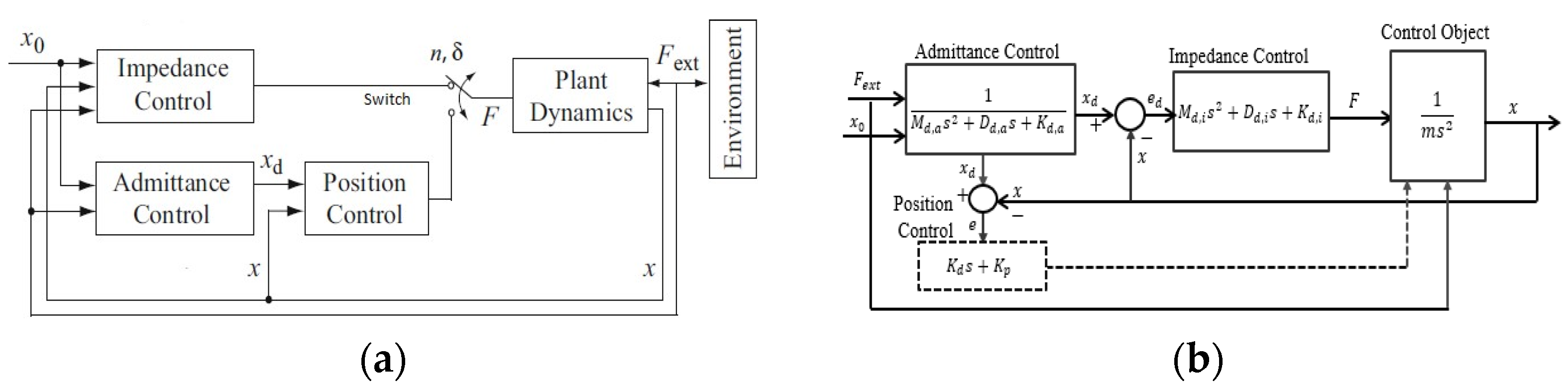
2.1. Parallel Structure with a Switched Framework
2.2. Series Structure without a Switched Framework
2.3. Interaction Force/Torque Sensorless Estimation
2.4. Conclusion
2.5. Research Contributions
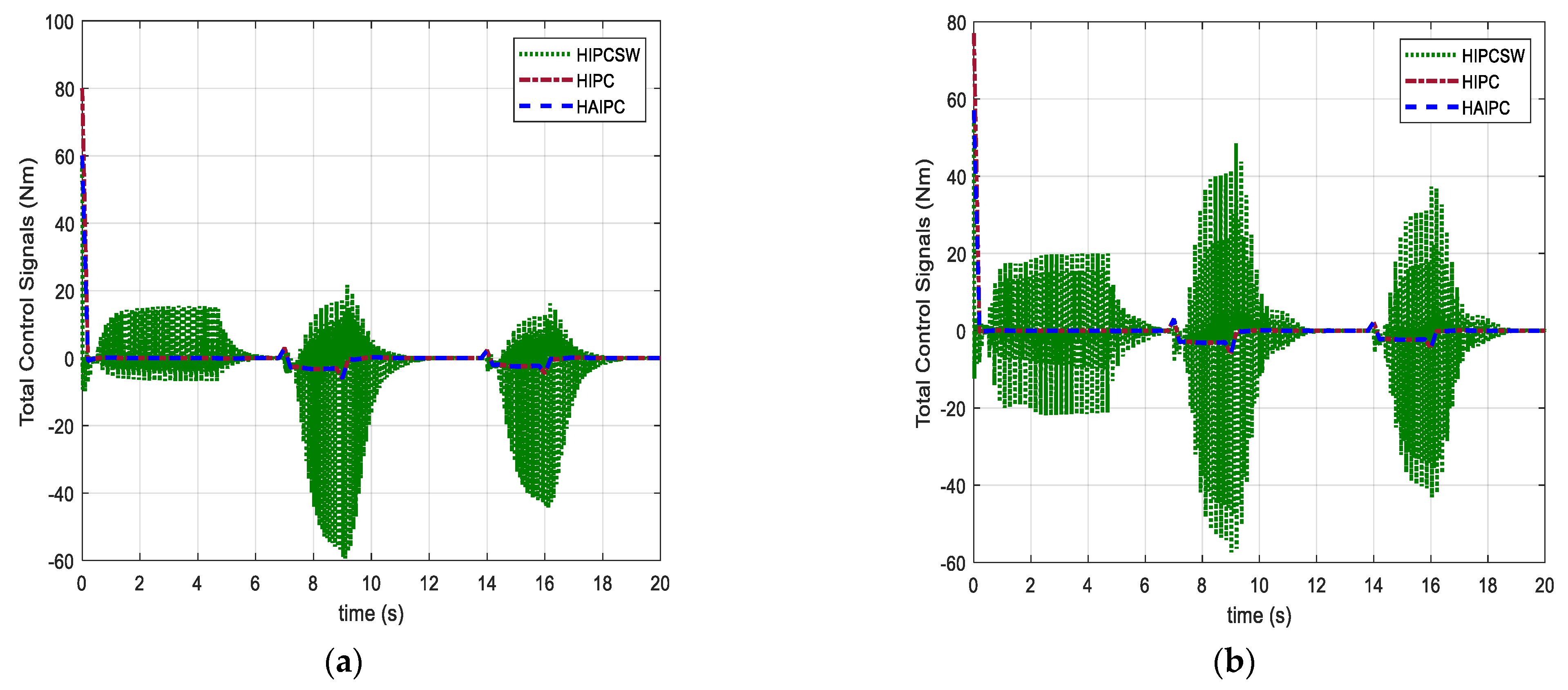
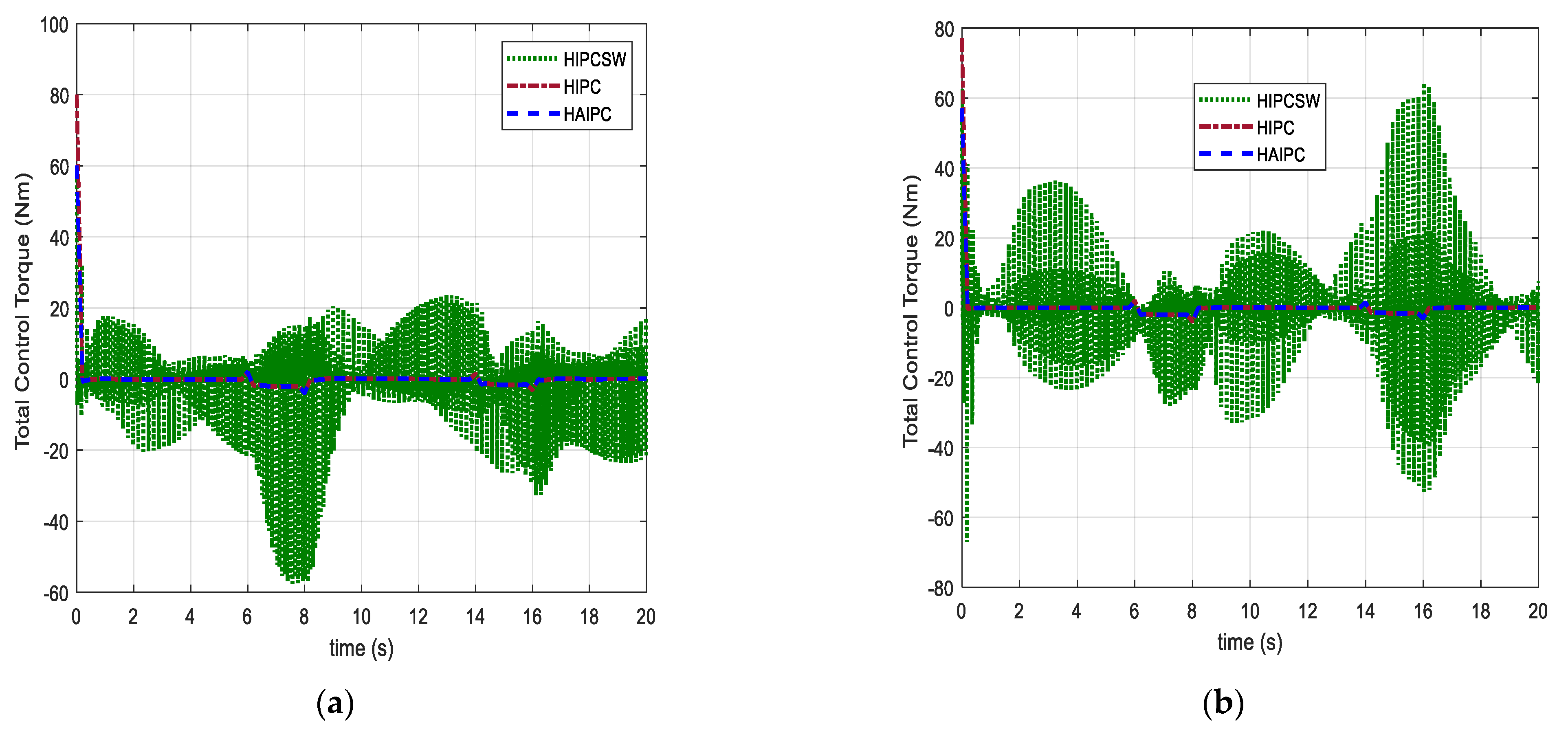
- The proposed method used the sensorless estimated interaction joint torque based on the actuator input torque of the system to update the stiffness and damping constants in the impedance control. This implies that the control torque due to impedance control is zero during soft contact, unlike the HIPC, which has high constant stiffness and damping gains both during soft and stiff contacts. Thus, the proposed method has low starting control input torque.
- The proposed method is adaptive and is designed based on series structure to avoid possible instability and chattering due to the switching process. Therefore, it combines the advantages of both HIPCSW and HIPC, namely low starting control input torque, the avoidance of instability and chattering effects, and low total control input torque consumption.
- To the best of our knowledge, based on the literature review, the proposed method is the first to use the sensorless estimation of interaction joint torque in the adaptive algorithm to update the stiffness and damping constant in the impedance control.
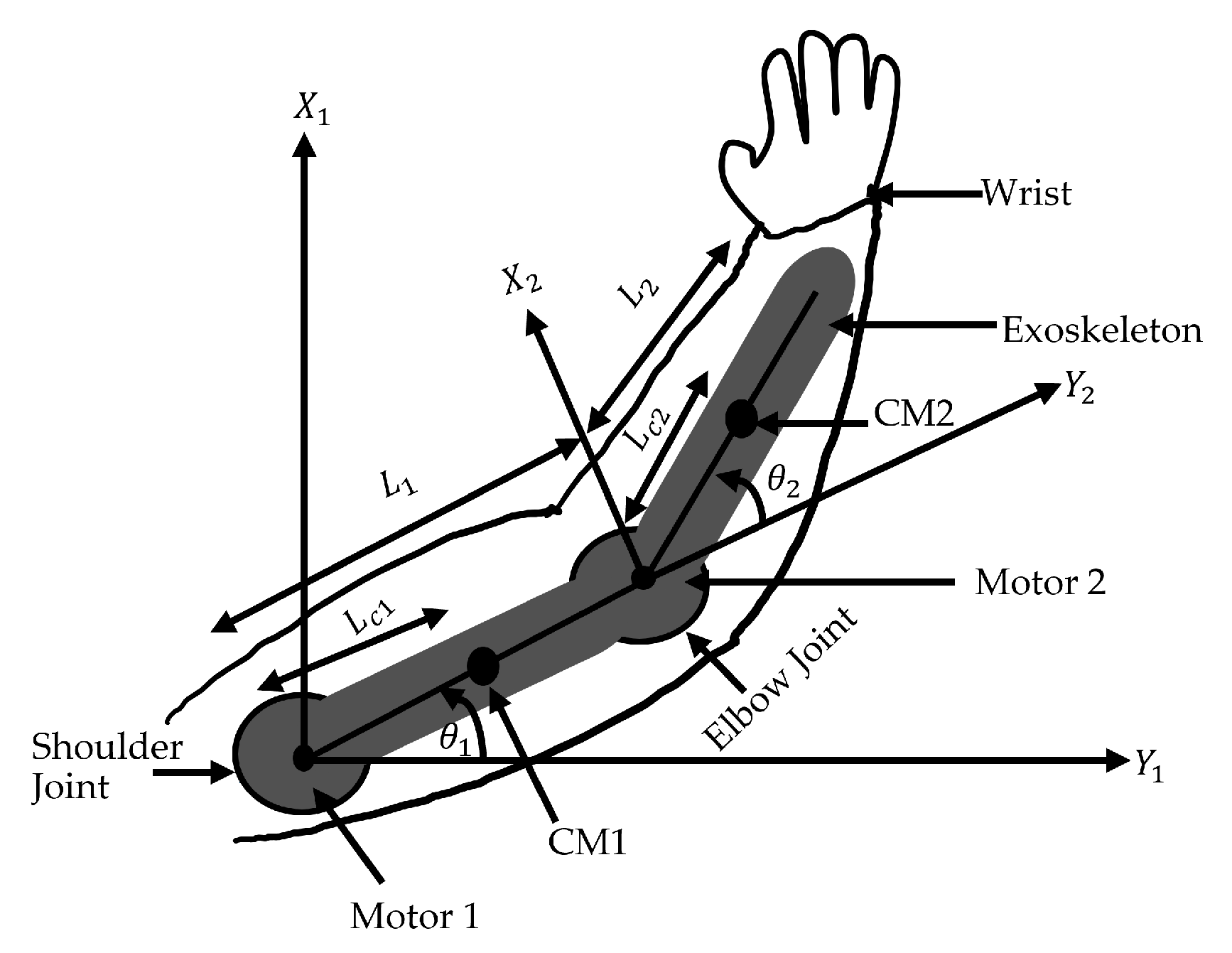
3. Mathematical Modelling
Nonlinear Model
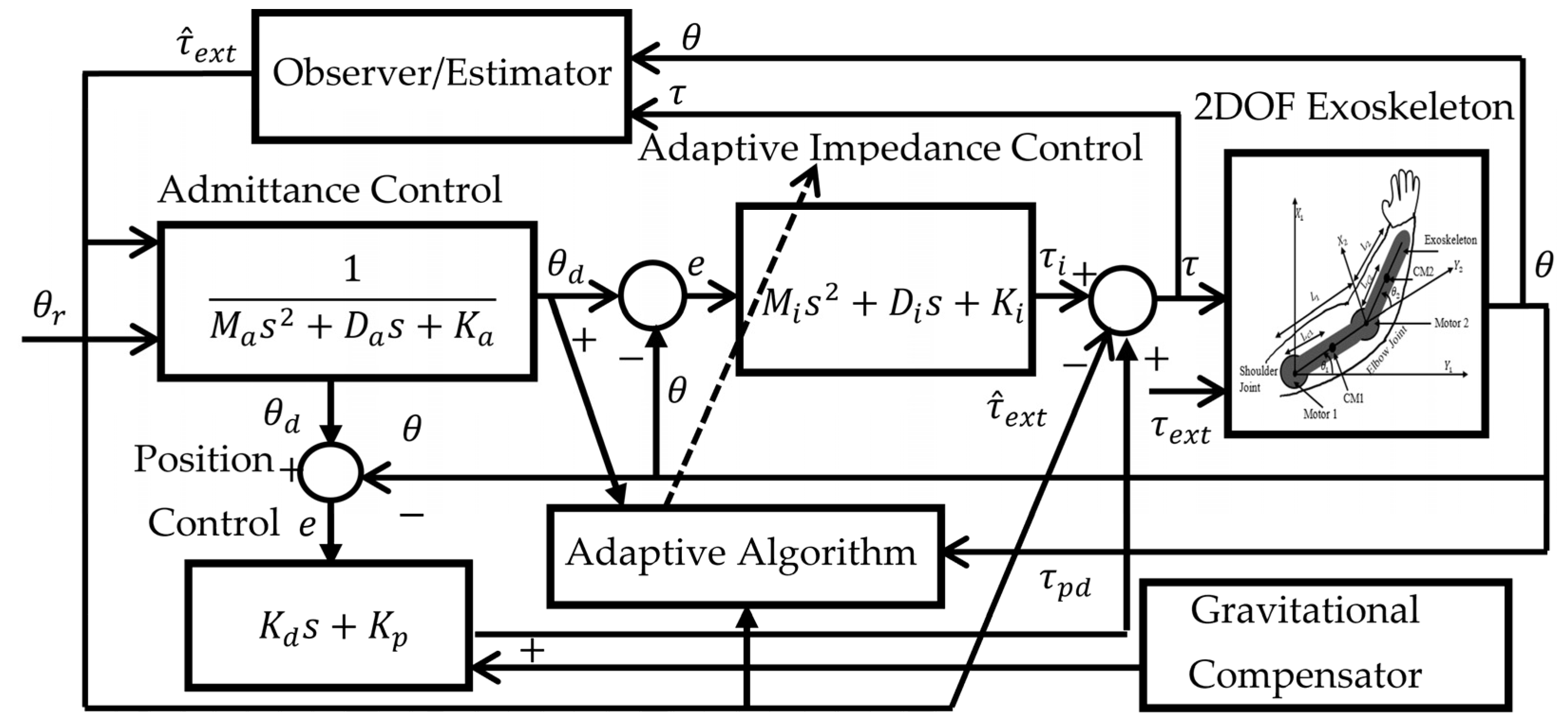
4. Control Design
4.1. PCGC Design
4.2. Interaction Joint Torque Estimation
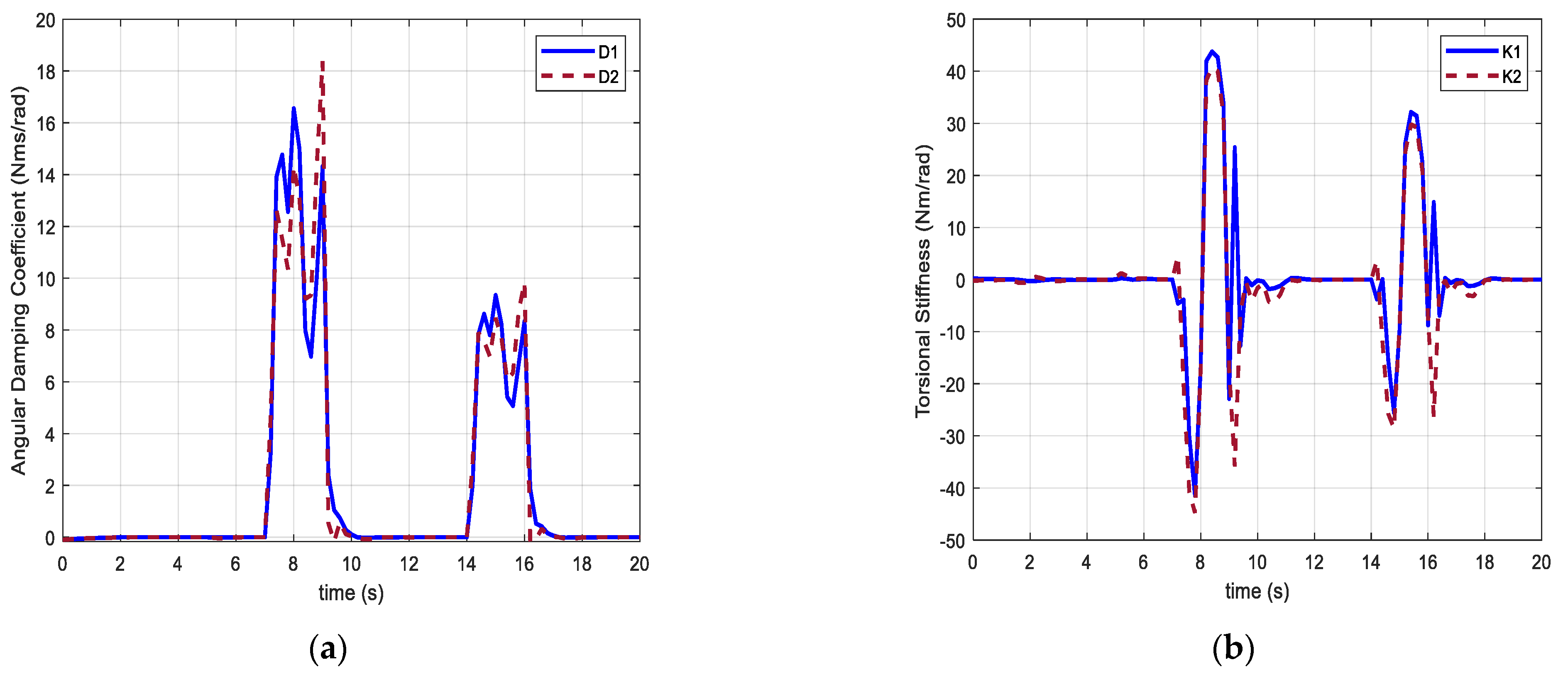
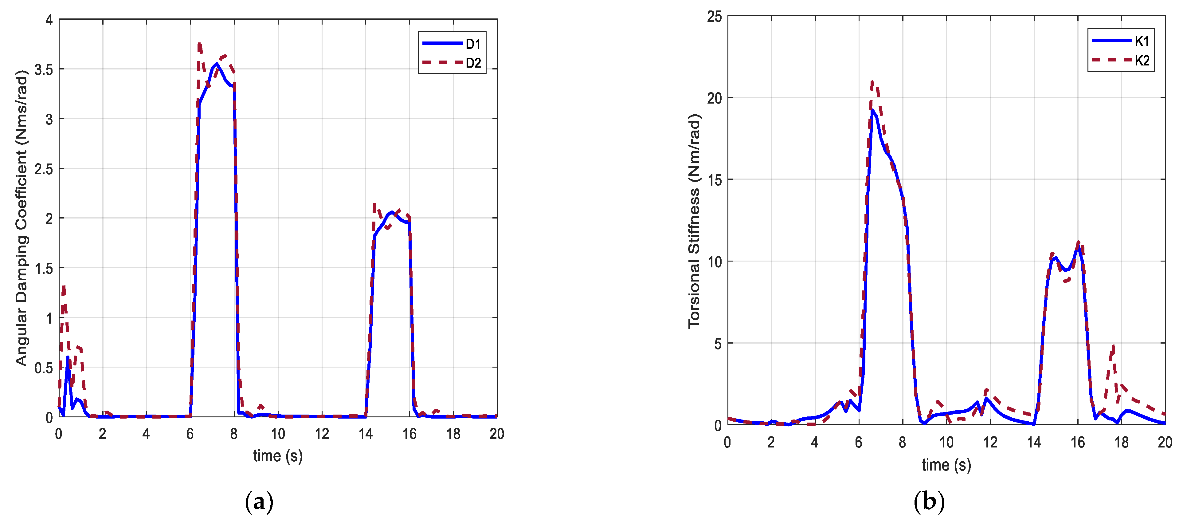
4.3. Adaptive Impedance Control
4.4. Stability Analysis
5. Results and Discussion
5.1. Setup
5.2. Simulation Results
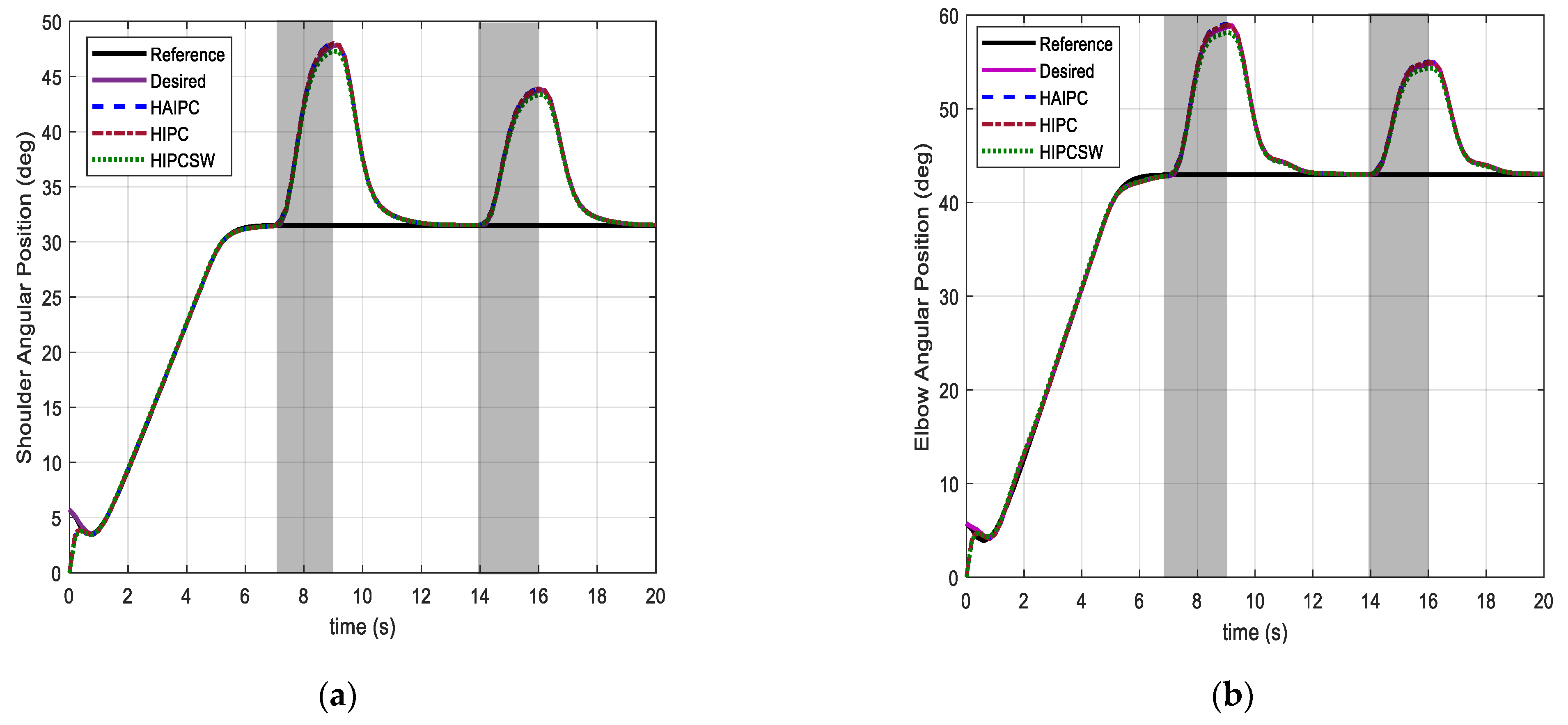
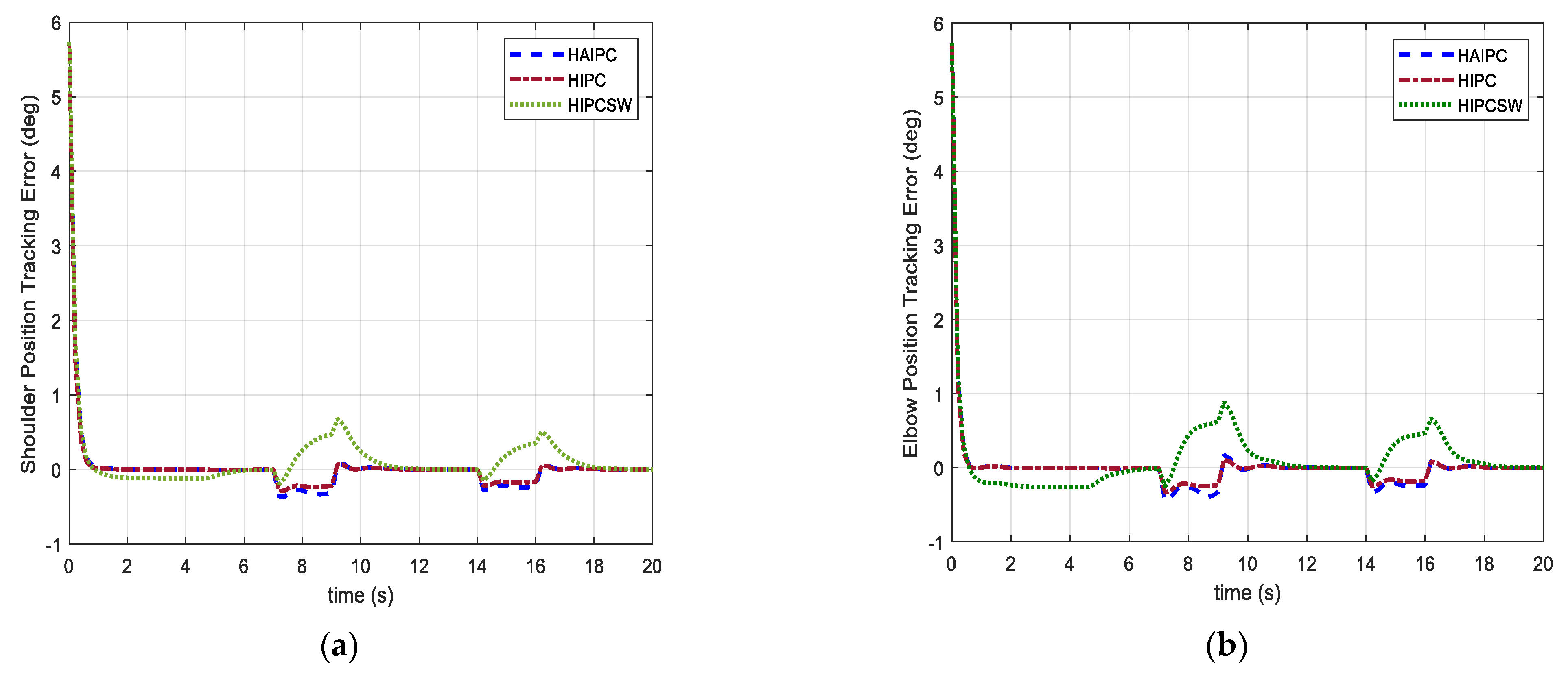
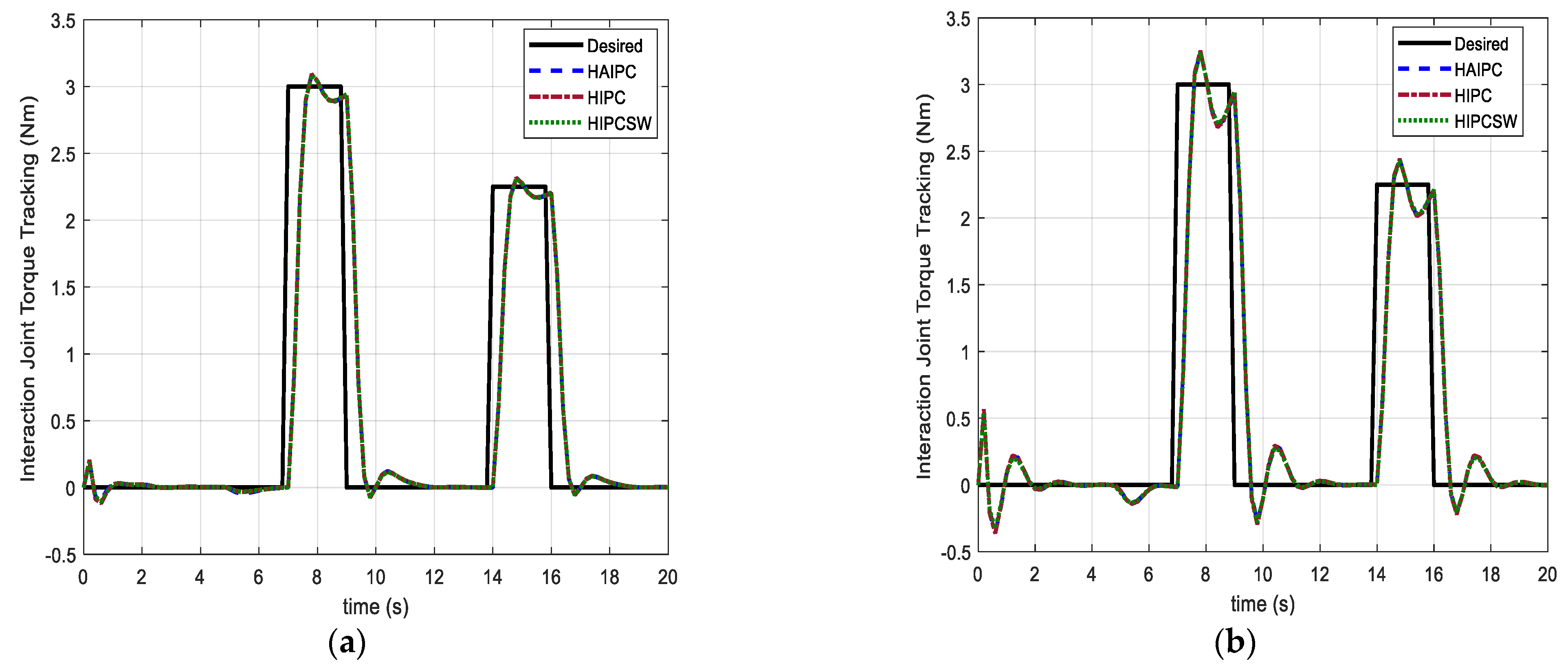
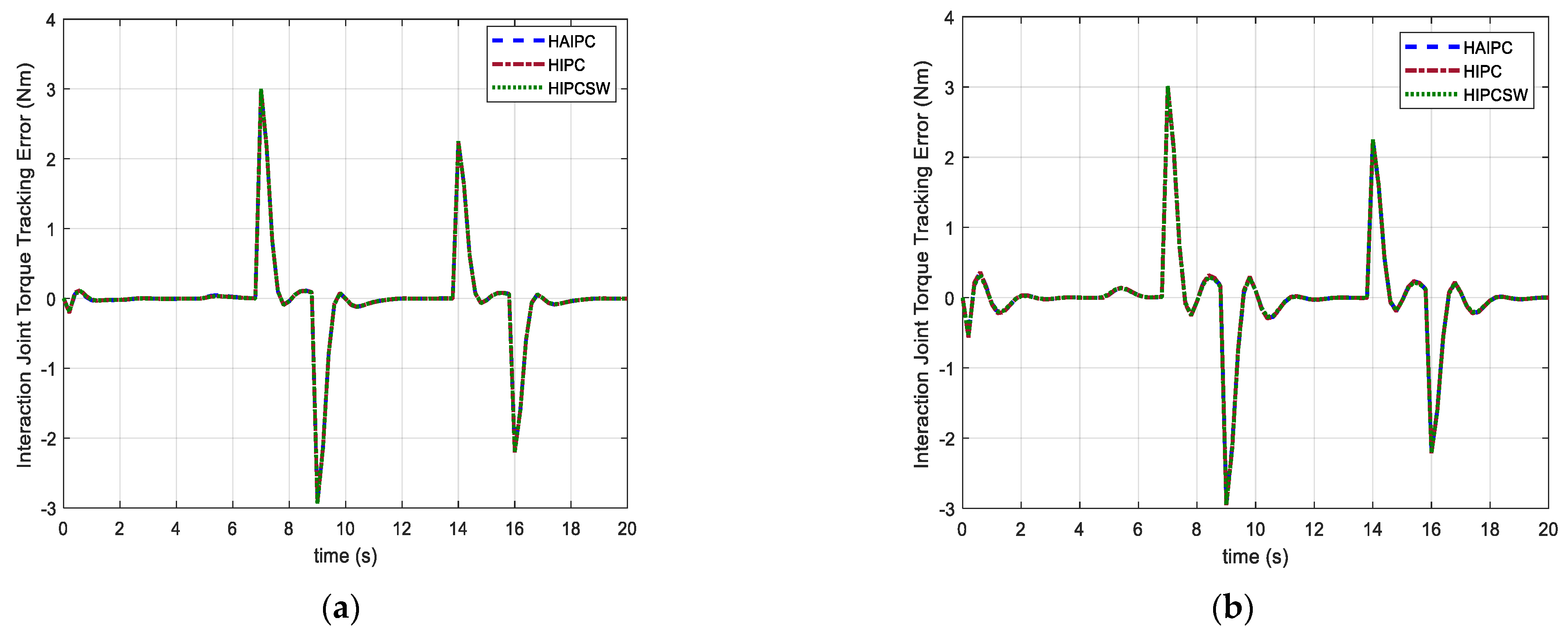
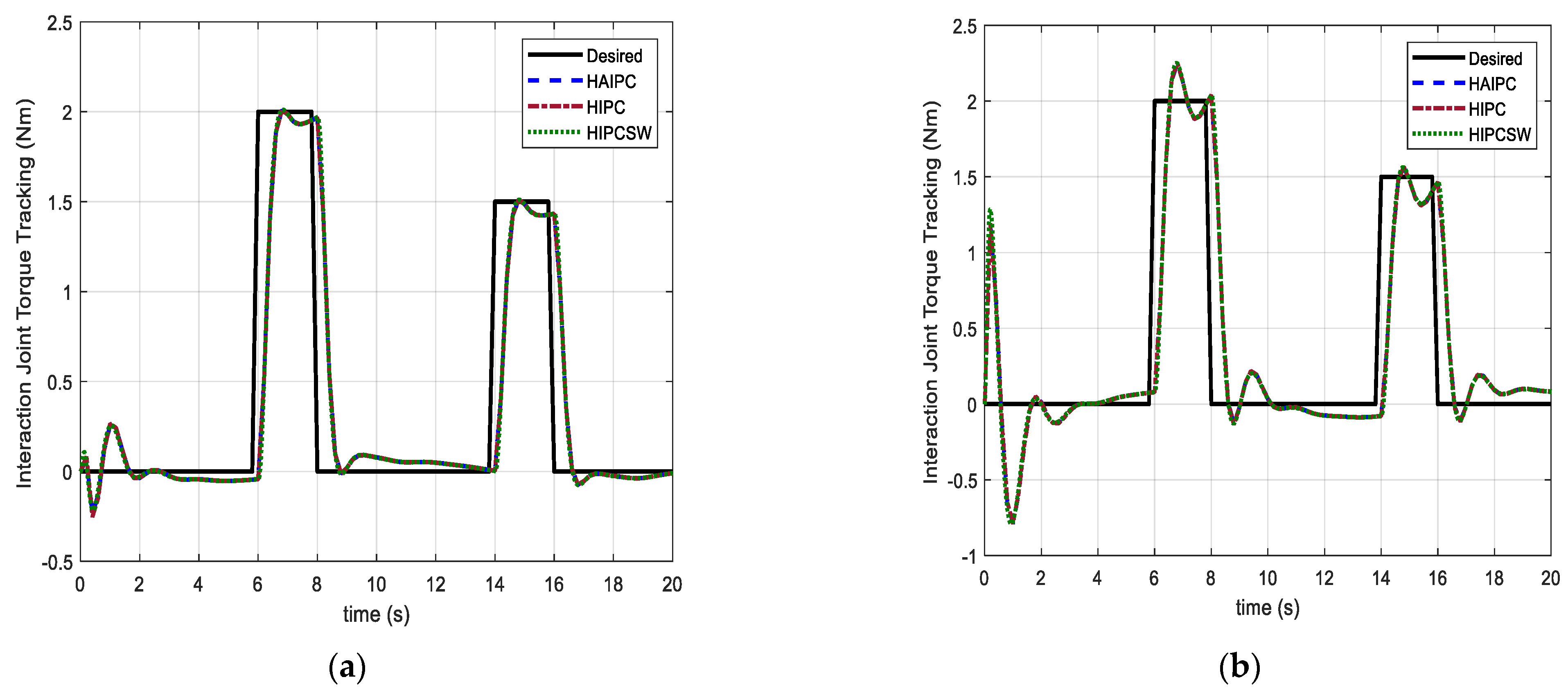
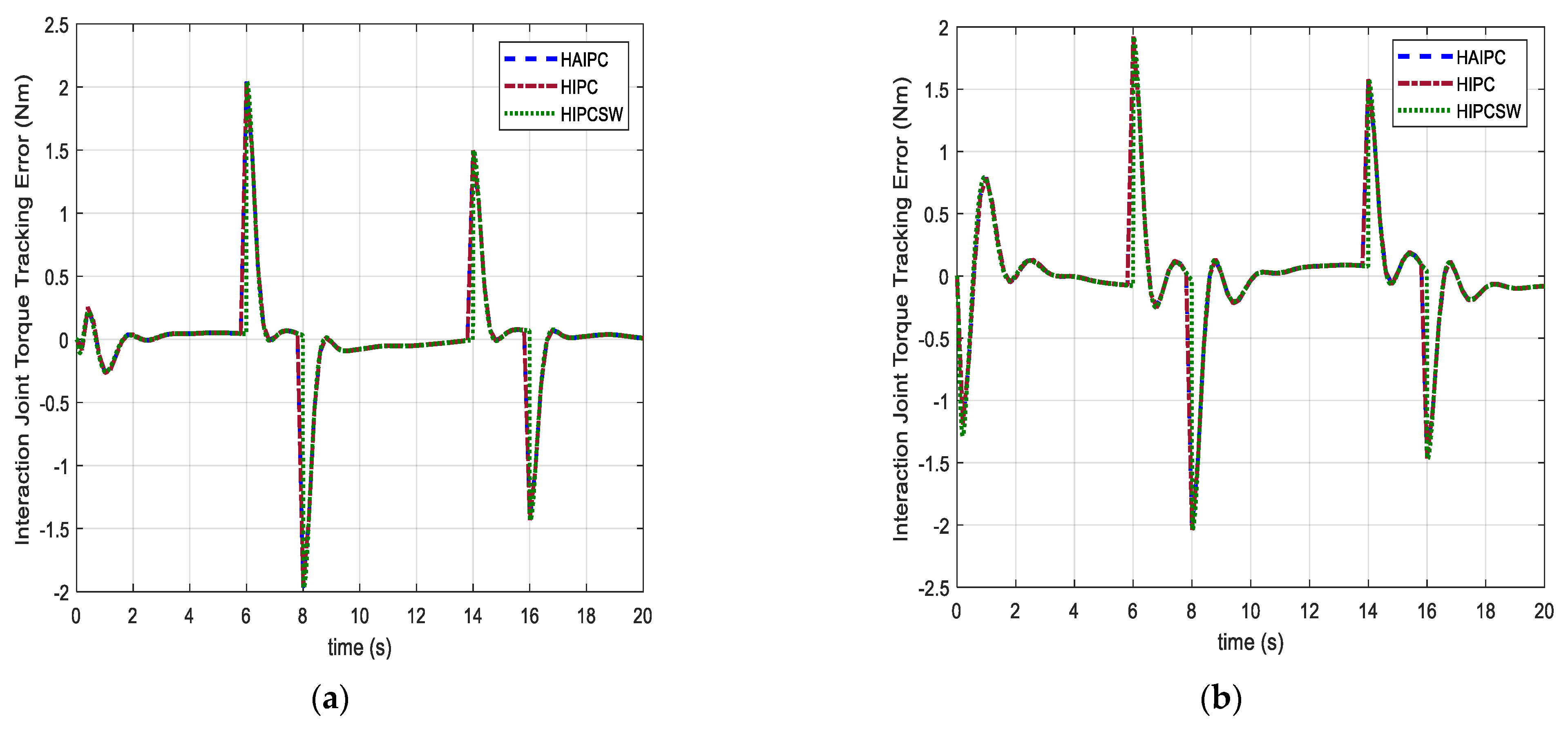
5.2.1. Case I: Isotonic Exercise
5.2.2. Case II: Active-Assistive Exercise
6. Conclusions
Author Contributions
Funding
Data Availability Statement
Acknowledgments
Conflicts of Interest
References
- Tantagunninat, T.; Wongkaewcharoen, N.; Pornpipatsakul, K.; Chuengpichanwanich, R.; Chaichaowarat, R. Modulation of joint stiffness for controlling the cartesian stiffness of a 2-DOF planar robotic arm for rehabilitation. In Proceedings of the 2023 IEEE/ASME International Conference on Advanced Intelligent Mechatronics, Seattle, WA, USA, 28–30 June 2023; pp. 598–603. [Google Scholar]
- Mesatien, T.; Suksawasdi, R.; Ayuthaya, N.; Chenviteesook, A.; Chaichaowarat, R. Position accuracy of a 6-DOF passive robotic arm for ultrasonography training. In Proceedings of the IEEE Region 10 Technical Conference, Chiang Mai, Thailand, 31 October–3 November 2023; pp. 841–846. [Google Scholar]
- Chaichaowarat, R.; Prakthong, S.; Thitipankul, S. Transformable wheelchair–exoskeleton hybrid robot for assisting human locomotion. Robotics 2023, 12, 16. [Google Scholar] [CrossRef]
- Chaichaowarat, R.; Macha, V.; Wannasuphoprasit, W. Passive knee exoskeleton using brake torque to assist stair ascent. In Proceedings of the IEEE Region 10 Technical Conference, Osaka, Japan, 16–19 November 2020; pp. 1165–1170. [Google Scholar]
- Chaichaowarat, R.; Nishimura, S.; Nozaki, T.; Krebs, H.I. Work in the time of COVID-19: Actuators and sensors for rehabilitation robotics. IEEJ J. Ind. Appl. 2021, 11, 256–265. [Google Scholar] [CrossRef]
- Chaichaowarat, R.; Nishimura, S.; Krebs, H.I. Design and modeling of a variable-stiffness spring mechanism for impedance modulation in physical human–robot interaction. In Proceedings of the 2021 IEEE International Conference on Robotics and Automation, Xi’an, China, 30 May–5 June 2021; pp. 7052–7057. [Google Scholar]
- Ullah, Z.; Chaichaowarat, R.; Wannasuphoprasit, W. Variable damping actuator using an electromagnetic brake for impedance modulation in physical human–robot interaction. Robotics 2023, 12, 80. [Google Scholar] [CrossRef]
- Hogan, N. Impedance Control: An Approach to Manipulation. In Proceedings of the American Control Conference, San Diego, CA, USA, 6–8 June 1984; pp. 304–313. [Google Scholar] [CrossRef]
- Hogan, N. The mechanics of multi-joint posture and movement control. Biol. Cybern. 1985, 52, 315–331. [Google Scholar] [CrossRef] [PubMed]
- Alexandre, R.; Emelie, S.; Marc, D. Enhancing Human Mobility Exoskeleton Comfort Using Admittance Controller. WSEAS Trans. Biol. Biomed. 2021, 18, 24–31. [Google Scholar] [CrossRef]
- Nyulangone Health. Available online: https://nyulangone.org/news/computer-tool-can-track-stroke-rehabilitation-boost-recovery (accessed on 17 February 2024).
- Arents, J.; Abolins, V.; Judvaitis, J.; Vismanis, O.; Oraby, A.; Ozols, K. Human–Robot Collaboration Trends and Safety Aspects: A Systematic Review. J. Sens. Actuator Netw. 2021, 10, 48. [Google Scholar] [CrossRef]
- Chiou, S.J.; Chu, H.R.; Li, I.H.; Lee, L.W. A Novel Wearable Upper-Limb Rehabilitation Assistance Exoskeleton System Driven by Fluidic Muscle Actuators. Electronics 2023, 12, 196. [Google Scholar] [CrossRef]
- Anderson, R.; Spong, M.W. Hybrid impedance control of robotic manipulators. IEEE J. Robot. Autom. 1988, 4, 549–556. [Google Scholar] [CrossRef]
- Ott, C.; Mukherjee, R.; Nakamura, Y.A. Hybrid System Framework for Unified Impedance and Admittance Control. J. Intell. Robot. Syst. 2015, 78, 359–375. [Google Scholar] [CrossRef]
- Liu, G.J.; Goldenberg, A.A. Robust hybrid impedance control of robot manipulators. In Proceedings of the 1991 IEEE International Conference on Robotics and Automation, Sacramento, CA, USA, 9–11 April 1991; pp. 287–292. [Google Scholar]
- Akdoaän, E.; Aktan, M.E.; Koru, A.T.; Arslan, M.S.; Atlıhan, M.; Kuran, B. Hybrid impedance control of a robot manipulator for wrist and forearm rehabilitation: Performance analysis and clinical results. Mechatronics 2018, 49, 77–91. [Google Scholar] [CrossRef]
- Kim, Y. Hybrid-Mode Impedance Control for Position/Force Tracking in Motor-System Rehabilitation. Int. J. Adv. Robot. Syst. 2015, 12, 79. [Google Scholar] [CrossRef]
- Ye, D.; Yang, C.; Jiang, Y.; Zhang, H. Hybrid impedance and admittance control for optimal robot–environment interaction. Robotica 2024, 42, 510–535. [Google Scholar] [CrossRef]
- Formenti, A.; Bucca, G.; Shahid, A.A.; Piga, D.; Roveda, L. Improved impedance/admittance switching controller for the interaction with a variable stiffness environment. Complex Eng. Syst. 2022, 2, 12. [Google Scholar] [CrossRef]
- Oh, Y.; Chung, W.K.; Youm, Y.; Suh, I.H. Motion/force decomposition of redundant manipulators and its application to hybrid impedance control. In Proceedings of the 1998 IEEE International Conference on Robotics and Automation, Leuven, Belgium, 16–20 May 1998; pp. 1441–1446. [Google Scholar]
- Wang, J.; Li, Y. Hybrid impedance control of a 3-DOF robotic arm used for rehabilitation treatment. In Proceedings of the 2010 IEEE International Conference on Automation Science and Engineering, Toronto, ON, Canada, 21–24 August 2010; pp. 768–773. [Google Scholar] [CrossRef]
- Ajani, O.S.; Assal, S.F.M. Hybrid Force Tracking Impedance Control-Based Autonomous Robotic System for Tooth Brushing Assistance of Disabled People. IEEE Trans. Med. Robot. Bionics 2020, 2, 649–660. [Google Scholar] [CrossRef]
- Rhee, I.; Kang, G.; Moon, S.J.; Choi, Y.S.; Choi, H.R. Hybrid impedance and admittance control of robot manipulator with unknown environment. Intell. Serv. Robot. 2023, 16, 49–60. [Google Scholar] [CrossRef]
- Ott, C.; Mukherjee, R.; Nakamura, Y. Unified Impedance and Admittance Control. In Proceedings of the 2010 IEEE International Conference on Robotics and Automation, Anchorage, AK, USA, 3–7 May 2010; pp. 554–561. [Google Scholar]
- Zhuang, Y.C.; Liu, Y.J.; Yu, W.S.; Lin, P.C. A Hybrid Impedance and Admittance Control Strategy for a Shape-Transformable Leg-Wheel. In Proceedings of the 2023 IEEE/ASME International Conference on Advanced Intelligent Mechatronics, Seattle, WA, USA, 27 June–1 July 2023; pp. 299–304. [Google Scholar] [CrossRef]
- da Silva, L.D.L.; Pereira, T.F.; Leithardt, V.R.Q.; Seman, L.O.; Zeferino, C.A. Hybrid Impedance-Admittance Control for Upper Limb Exoskeleton Using Electromyography. Appl. Sci. 2020, 10, 7146. [Google Scholar] [CrossRef]
- Cetin, K.; Zapico, C.S.; Tugal, H.; Petillot, Y.; Dunnigan, M.; Erden, M.S. Application of Adaptive and Switching Control for Contact Maintenance of a Robotic Vehicle-Manipulator System for Underwater Asset Inspection. Front. Robot. AI 2021, 8, 706558. [Google Scholar] [CrossRef]
- Jiao, C.; Yu, L.; Su, X.; Wen, Y.; Dai, X. Adaptive hybrid impedance control for dual-arm cooperative manipulation with object uncertainties. Automatica 2022, 140, 110232. [Google Scholar] [CrossRef]
- Cavenago, F.; Voli, L.; Massari, M. Adaptive hybrid system framework for unified impedance and admittance control. J. Intell. Robot. Syst. 2018, 91, 569–581. [Google Scholar] [CrossRef]
- Sun, T.; Wang, Z.; He, C.; Yang, L. Adaptive Robust Admittance Control of Robots Using Duality Principle-Based Impedance Selection. Appl. Sci. 2022, 12, 12222. [Google Scholar] [CrossRef]
- Cao, H.; He, Y.; Chen, X.; Zhao, X. Smooth adaptive hybrid impedance control for robotic contact force tracking in dynamic environments. Ind. Robot 2020, 47, 231–242. [Google Scholar] [CrossRef]
- Ding, S.; Peng, J.; Zhang, H.; Wang, Y. Neural network-based adaptive hybrid impedance control for electrically driven flexible-joint robotic manipulators with input saturation. Neurocomputing 2021, 458, 99–111. [Google Scholar] [CrossRef]
- Moughamir, S.; Eneve, A.; Zaytoon, J.; Afilal, L. Hybrid Force/Impedance Control for the Robotiled Rehabilitation of the Upper Limbs. In Proceedings of the 16th IFAC World Congress, Prague, Czech Republic, 3–8 July 2005; Volume 38. [Google Scholar] [CrossRef]
- Fujiki, T.; Tahara, K. Series admittance–impedance controller for more robust and stable extension of force control. Robomech. J. 2022, 9, 23. [Google Scholar] [CrossRef]
- Kitchatr, S.; Sirimangkalalo, A.; Chaichaowarat, R. Visual servo control for ball-on-plate balancing: Effect of PID controller gain on tracking performance. In Proceedings of the 2023 IEEE International Conference on Robotics and Biomimetics, Koh Samui, Thailand, 4–9 December 2023; pp. 1–6. [Google Scholar]
- Bätz, G.; Weber, B.; Scheint, M.; Wollherr, D.; Buss, M. Dynamic contact force/torque observer: Sensor fusion for improved interaction control. Int. J. Robot. Res. 2013, 32, 446–457. [Google Scholar] [CrossRef]
- Jung, J.; Lee, J.; Huh, K. Robust contact force estimation for robot manipulators in three-dimensional space. Proc. Inst. Mech. Eng. Part C J. Mech. Eng. Sci. 2006, 220, 1317–1327. [Google Scholar] [CrossRef]
- Birjandi, S.A.B.; Khurana, H.; Billard, A.; Haddadin, S. A Stable Adaptive Extended Kalman Filter for Estimating Robot Manipulators Link Velocity and Acceleration. In Proceedings of the 2023 IEEE/RSJ International Conference on Intelligent Robots and Systems, Detroit, MI, USA, 1–5 October 2023; pp. 346–353. [Google Scholar] [CrossRef]
- Yousefizadeh, S.; Bak, T. Unknown External Force Estimation and Collision Detection for a Cooperative Robot. Robotica 2020, 38, 1665–1681. [Google Scholar] [CrossRef]
- Feng, C.; Docherty, P.D.; Ni, S.; Chen, X. Contact force and torque sensing for serial manipulator based on an adaptive Kalman filter with variable time period. Robot. Comput.-Integr. Manuf. 2021, 72, 102210. [Google Scholar] [CrossRef]
- Dong, J.; Xu, J.; Wang, L.; Liu, A.; Yu, L. External force estimation of the industrial robot based on the error probability model and SWVAKF. IEEE Trans. Instrum. Meas. 2022, 71, 1–11. [Google Scholar] [CrossRef]
- Chen, C.; Zhang, C.; Hu, T.; Ni, H.; Luo, W. Model-assisted extended state observer-based computed torque control for trajectory tracking of uncertain robotic manipulator systems. Int. J. Adv. Robot. Syst. 2018, 15, 1729881418801738. [Google Scholar] [CrossRef]
- Gijo, S.; Zeyu, L.; Vincent, C.; Demy, K.; Ying, T.; Denny, O. Interaction Force Estimation Using Extended State Observers: An Application to Impedance-Based Assistive and Rehabilitation Robotics. IEEE Robot. Autom. Lett. 2019, 4, 1156–1161. [Google Scholar]
- Abdullahi, A.M.; Chaichaowarat, R. Sensorless Estimation of Human Joint Torque for Robust Tracking Control of Lower-Limb Exoskeleton Assistive Gait Rehabilitation. J. Sens. Actuator Netw. 2023, 12, 53. [Google Scholar] [CrossRef]
- Chan, L.; Fazel, N.; David, S. Extended active observer for force estimation and disturbance rejection of robotic manipulators. Robot. Auton. Syst. 2013, 61, 1277–1287. [Google Scholar] [CrossRef]
- Li, T.; Xing, H.; Hashemi, E.; Taghirad, H.D.; Tavakoli, M. A brief survey of observers for disturbance estimation and compensation. Robotica 2023, 41, 3818–3845. [Google Scholar] [CrossRef]
- Zhao, J.; Yang, T.; Sun, X.; Dong, J.; Wang, Z.; Yang, C. Sliding mode control combined with extended state observer for an ankle exoskeleton driven by electrical motor. Mechatronics 2021, 76, 102554. [Google Scholar] [CrossRef]
- Zhang, J.; Gao, W.; Guo, Q. Extended State Observer-Based Sliding Mode Control Design of Two-DOF Lower Limb Exoskeleton. Actuators 2023, 12, 402. [Google Scholar] [CrossRef]
- Ren, T.; Dong, Y.; Wu, D.; Chen, K. Impedance control of collaborative robots based on joint torque servo with active disturbance rejection. Ind. Robot 2019, 46, 518–528. [Google Scholar] [CrossRef]
- Liu, X.; Zuo, G.; Zhang, J.; Wang, J. Sensorless force estimation of end-effect upper limb rehabilitation robot system with friction compensation. Int. J. Adv. Robot. Syst. 2019, 16, 1729881419856132. [Google Scholar] [CrossRef]
- Liang, W.; Huang, S.; Chen, S.; Tan, K.K. Force estimation and failure detection based on disturbance observer for an ear surgical device. ISA Trans. 2017, 66, 476–484. [Google Scholar] [CrossRef] [PubMed]
- Qin, J.; Léonard, F.; Abba, G. Experimental external force estimation using a non-linear observer for 6 axes flexible-joint industrial manipulators. In Proceedings of the 2013 9th Asian Control Conference (ASCC), Istanbul, Turkey, 23–26 June 2013; pp. 1–6. [Google Scholar] [CrossRef]
- Kružić, S.; Musić, J.; Kamnik, R.; Papić, V. End-Effector Force and Joint Torque Estimation of a 7-DoF Robotic Manipulator Using Deep Learning. Electronics 2021, 10, 23. [Google Scholar] [CrossRef]
- Kaya, O.; Yildirim, M.C.; Kuzuluk, N.; Cicek, E.; Bebek, O.; Oztop, E.; Ugurlu, B. Environmental force estimation for a robotic hand: Compliant contact detection. In Proceedings of the 2015 IEEE-RAS 15th International Conference on Humanoid Robots (Humanoids), Seoul, Republic of Korea, 3–5 November 2015; pp. 791–796. [Google Scholar] [CrossRef]
- Alcocer, A.; Robertsson, A.; Valera, A.; Johansson, R. Force estimation and control in robot manipulators. IFAC Proc. Vol. 2003, 36, 55–60. [Google Scholar] [CrossRef]
- Colomé, A.; Pardo, D.; Alenyà, G.; Torras, C. External force estimation during compliant robot manipulation. In Proceedings of the 2013 IEEE International Conference on Robotics and Automation, Karlsruhe, Germany, 6–10 May 2013; pp. 3535–3540. [Google Scholar] [CrossRef]
- Liu, S.; Wang, L.; Wang, X.V. Sensorless force estimation for industrial robots using disturbance observer and neural learning of friction approximation. Robot. Comput.-Integr. Manuf. 2021, 71, 102168. [Google Scholar] [CrossRef]
- Loris, R.; Dario, P. Sensorless environment stiffness and interaction force estimation for impedance control tuning in robotized interaction tasks. Auto Robot. 2021, 45, 371–388. [Google Scholar] [CrossRef]
- Aole, S.; Elamvazuthi, I.; Waghmare, L.; Patre, B.; Bhaskarwar, T.; Meriaudeau, F.; Su, S. Active Disturbance Rejection Control Based Sinusoidal Trajectory Tracking for an Upper Limb Robotic Rehabilitation Exoskeleton. Appl. Sci. 2022, 12, 1287. [Google Scholar] [CrossRef]
- Kronander, K.; Billard, A. Stability Considerations for Variable Impedance Control. IEEE Trans. Robot. 2016, 32, 1298–1305. [Google Scholar] [CrossRef]


| Control Methods | Advantages | Disadvantages |
|---|---|---|
| Parallel Structure (i.e., HIPCSW) |
|
|
| Series Structure (i.e., HIPC) |
|
|
| Parameters | Symbols | Values | Units |
|---|---|---|---|
| Mass of the Upper Arm Limb | 2.25 | kg | |
| Mass of the Lower Arm Limb | 1.47 | kg | |
| Upper Arm Length | 0.34 | m | |
| Lower Arm Length | 0.25 | m | |
| Distance from Shoulder to Upper Arm CM | 0.17 | m | |
| Distance from Elbow to Lower Arm CM | 0.125 | m | |
| Mass Moment of Inertia about the Shoulder Joint | 0.2505 | kg × m2 | |
| Mass Moment of Inertia about the Elbow Joint | 0.0925 | kg × m2 |
| Control Method | Position Tracking MAE (Degree) | Torque Tracking MAE (Nm) | Control Torque MAV (Nm) | |||
|---|---|---|---|---|---|---|
| Shoulder | Elbow | Shoulder | Elbow | Shoulder | Elbow | |
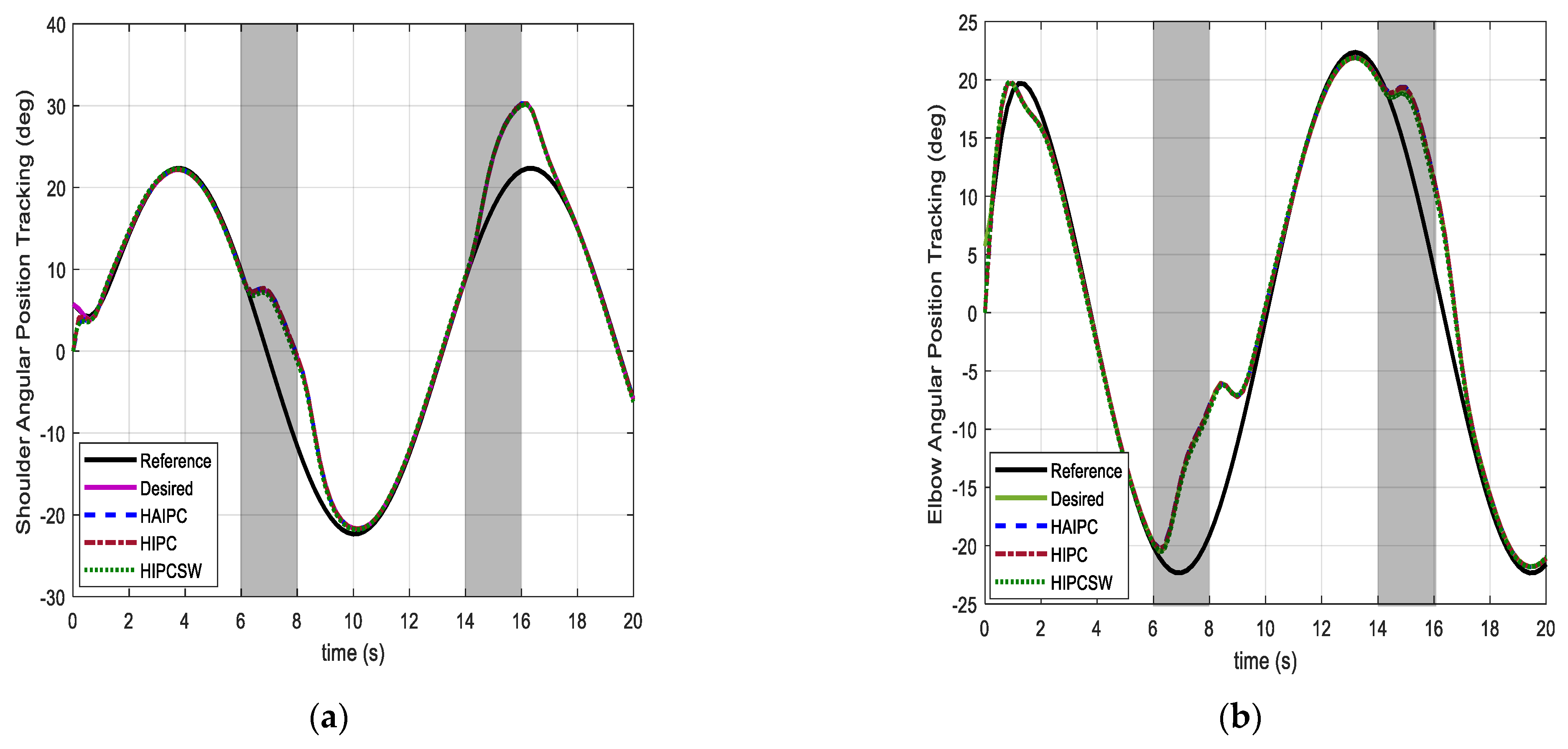
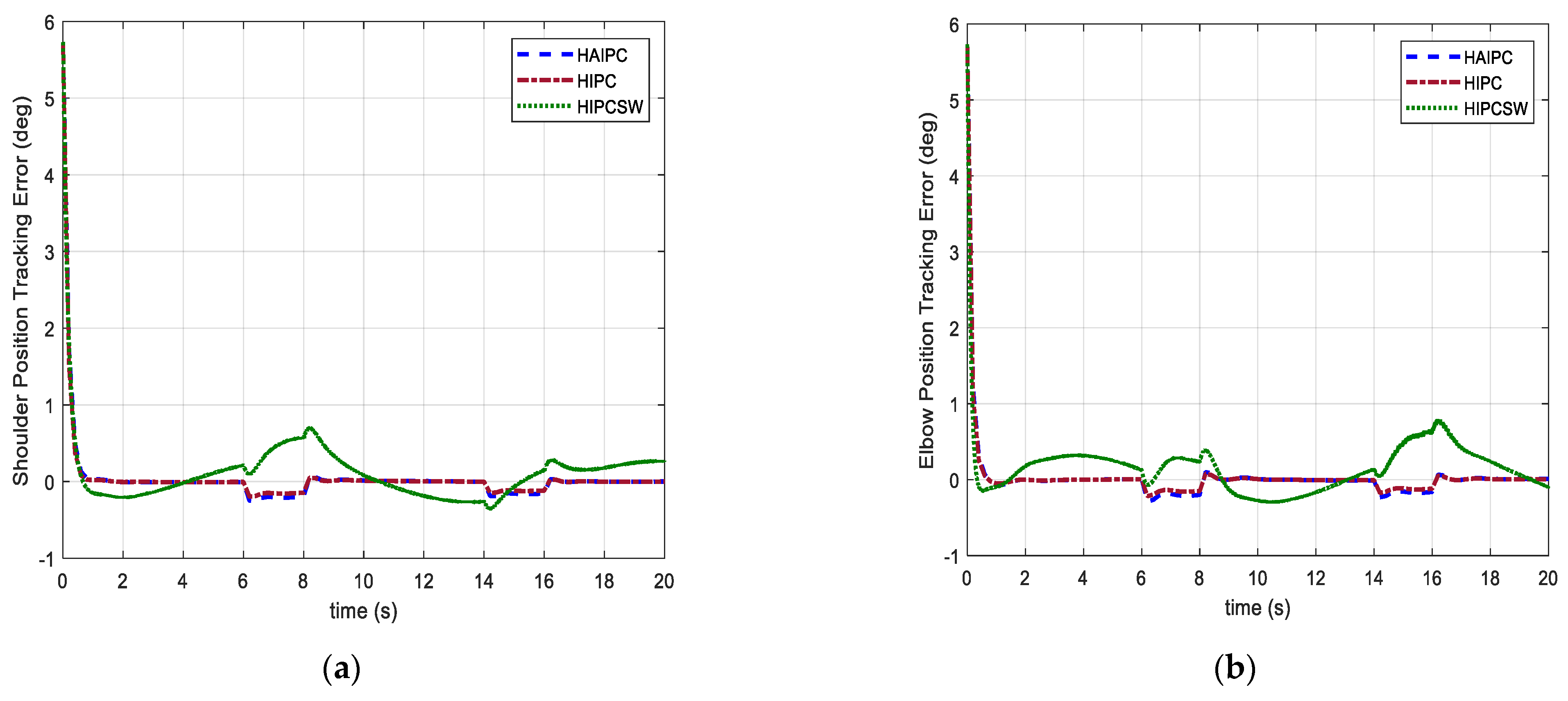
| HAIPC | 0.1412 | 0.1388 | 0.2345 | 0.2783 | 1.2685 | 1.2112 |
| HIPC | 0.1232 | 0.1198 | 0.2352 | 0.2801 | 1.4692 | 1.4093 |
| HIPCSW | 0.2045 | 0.2610 | 0.2348 | 0.2755 | 8.1502 | 13.6272 |
| Control Method | Position Tracking MAE (Degree) | Torque Tracking MAE (Nm) | Control Torque MAV (Nm) | |||
|---|---|---|---|---|---|---|
| Shoulder | Elbow | Shoulder | Elbow | Shoulder | Elbow | |
| HAIPC | 0.1258 | 0.1212 | 0.1829 | 0.2409 | 1.0625 | 1.0025 |
| HIPC | 0.1101 | 0.1075 | 0.1836 | 0.2413 | 1.2604 | 1.2000 |
| HIPCSW | 0.2784 | 0.2996 | 0.1820 | 0.2407 | 13.3488 | 23.4849 |
| Parameters | Symbols |
|---|---|
| Centre of mass of link 1 | |
| Centre of mass of link 2 | |
| Inertia matrix | |
| Centrifugal and Coriolis torque | |
| Gravitational torque | |
| External torque | |
| Shoulder control torque | |
| Elbow control torque | |
| Proportional derivative (PD) position control torque | |
| Impedance torque | |
| Estimated interaction joint torque | |
| Shoulder joint observer gains | |
| Elbow joint observer gains | |
| Observer frequency | |
| Inertia constant of the impedance control | |
| Damping constant of the impedance control | |
| Stiffness constant of the impedance control | |
| Inertia constant of the admittance control | |
| Damping constant of the admittance control | |
| Stiffness constant of the admittance control | |
| Proportional gain of the PD controller | |
| Derivative gain of the PD controller | |
| Estimation vector | |
| Regression vector | |
| Covariance matrix | |
| Proportional derivative | PD |
| Genetic algorithm proportional derivative | GA_PD |
| Extended state observer | ESO |
| Recursive least-squares | RLS |
| Hybrid adaptive impedance position control | HAIPC |
| Hybrid impedance position control | HIPC |
| Hybrid impedance position control with switch | HIPCSW |
| Mean absolute error | MAE |
| Mean absolute value | MAV |
Disclaimer/Publisher’s Note: The statements, opinions and data contained in all publications are solely those of the individual author(s) and contributor(s) and not of MDPI and/or the editor(s). MDPI and/or the editor(s) disclaim responsibility for any injury to people or property resulting from any ideas, methods, instructions or products referred to in the content. |
© 2024 by the authors. Licensee MDPI, Basel, Switzerland. This article is an open access article distributed under the terms and conditions of the Creative Commons Attribution (CC BY) license (https://creativecommons.org/licenses/by/4.0/).
Share and Cite
Abdullahi, A.M.; Haruna, A.; Chaichaowarat, R. Hybrid Adaptive Impedance and Admittance Control Based on the Sensorless Estimation of Interaction Joint Torque for Exoskeletons: A Case Study of an Upper Limb Rehabilitation Robot. J. Sens. Actuator Netw. 2024, 13, 24. https://doi.org/10.3390/jsan13020024
Abdullahi AM, Haruna A, Chaichaowarat R. Hybrid Adaptive Impedance and Admittance Control Based on the Sensorless Estimation of Interaction Joint Torque for Exoskeletons: A Case Study of an Upper Limb Rehabilitation Robot. Journal of Sensor and Actuator Networks. 2024; 13(2):24. https://doi.org/10.3390/jsan13020024
Chicago/Turabian StyleAbdullahi, Auwalu Muhammad, Ado Haruna, and Ronnapee Chaichaowarat. 2024. "Hybrid Adaptive Impedance and Admittance Control Based on the Sensorless Estimation of Interaction Joint Torque for Exoskeletons: A Case Study of an Upper Limb Rehabilitation Robot" Journal of Sensor and Actuator Networks 13, no. 2: 24. https://doi.org/10.3390/jsan13020024