iMASKO: A Genetic Algorithm Based Optimization Framework for Wireless Sensor Networks

Abstract

In this paper we present the design and implementation of a generic GA-based optimization framework iMASKO (iNL@MATLAB Genetic Algorithm-based Sensor NetworK Optimizer) to optimize the performance metrics of wireless sensor networks. Due to the global search property of genetic algorithms, the framework is able to automatically and quickly fine tune hundreds of possible solutions for the given task to find the best suitable tradeoff. We test and evaluate the framework by using it to explore a SystemC-based simulation process to tune the configuration of the unslotted CSMA/CA algorithm of IEEE 802.15.4, aiming to discover the most available tradeoff solutions for the required performance metrics. In particular, in the test cases different sensor node platforms are under investigation. A weighted sum based cost function is used to measure the optimization effectiveness and capability of the framework. In the meantime, another experiment is performed to test the framework’s optimization characteristic in multi-scenario and multi-objectives conditions.

1. Introduction

With the widespread development of embedded systems and various wireless communication technologies, wireless sensor networks (WSNs) have gained the attention of industrial and research groups all over the world in recent years. The integration of sensing, data processing, and over-the-air transmission into a single miniaturized device enables the deployment of wireless sensor networks in many fields of applications. However, the weak computation ability, limited storage, short communication range, and severe energy constraints, to some extent, limit their use. Therefore, carrying out optimizations on these elements is very useful for the improvement of network lifetime, the reduction of packet loss, end-to-end delay, and other related metrics, all of which are essential to guarantee adequate performance for specific applications. Typically, two classes of objects are optimized in the design of wireless sensor networks: hardware and software.

From the hardware perspective, better energy efficiency can be achieved by optimizing the power consumption of related hardware components. By employing an ultra-low power based microcontroller (e.g., MSP430) and configuring it to five different low power modes, a significant amount of energy can be saved. Besides, the reduction of sensing tasks and simplification of data processing algorithms can also be helpful. For the transceiver, some factors, such as the modulation scheme, transceiver packet frame, and duty cycle, can affect power consumption. The use of a high data rate as described in [1], has proven to be, not only a very energy-effective choice, but also a strategy that greatly improves network reliability. In recent years, some emerging radio-based technologies such as Bluetooth low energy technology [2], Ultra-wideband (UWB) [3], and ANT [4] have also provided excellent choices in lifetime improvement, reliability enhancement, as well as short network latency. From the viewpoint of energy supply, as most sensor motes are battery-driven, the battery type, capacity, and size play an important role in the node lifetime, cost, weight, and deployment ability. Emerging energy harvesting technologies [5] are also highly useful methods for overall energy optimization and power management. In addition, some hardware based algorithms have been proposed for optimizing energy consumption. An adaptive power control algorithm is presented and implemented in [6], by automatically configuring the programmable output power on a transceiver chip according to the distance information between nodes. This algorithm is tested via experiment for the validation of its energy-efficiency in increasing node lifetime. A Dynamic Voltage Scaling (DVS) algorithm [7] applied to microprocessors can also minimize the power consumption by dynamically scaling the supply voltage to match the required performance level. Finally, in the Dynamic Power Management (DPM) algorithm [8], a more traditional method is used by selectively turning off idle state components to save energy.

From the software perspective, the optimization method can be grouped into three categories: the development of new communication protocols (MAC and routing) for optimization, the adoption of energy-aware strategies for optimization, and the configuration/exploration of the optimal set of existing protocols for optimization. Firstly, building on the contention-based scheme for collision avoidance and reliable transmission, both S-MAC [9] and T-MAC [10] are proposed to synchronize communication schedules and listening periods to minimize latency, while reducing energy consumption by turning off the radios during sleep periods. Through the use of low-power listening approaches, WiseMAC [11] and B-MAC [12] can save more energy from idle listening. For most of the new proposed routing protocols, optimizations focus on how to select the shortest path for energy saving, while, at the same time, guaranteeing the reliability of the network by reducing the number of communication hops. Secondly, the uses of strategies for optimization include in-network processing, data aggregation, and cross-layer related optimization methods. In-network processing in wireless sensor networks typically involves operations such as data compression and fusion. Despite the cost of increased latency (more time is spent in data processing), the impacts of this approach on energy reduction in [13] are always found to be significant. The idea of data aggregation is to gather the data from different source nodes to be forwarded onto further destination nodes, and is considered as an essential part in routing protocols of wireless sensor networks as it directly aims at reducing the amount of data to be transported. A data aggregation based method derived from compressed sensing (CS) is proposed in [14] to minimize the total energy consumption in the sensory data collecting process. Overall, the aggregation process helps eliminate redundancy from packet overhead, minimize the number of transmissions, and thus save total energy [15]. By exploiting the interactions between different layers of WSNs, cross-layer optimization techniques are able to improve energy conservation. In [16], taking both MAC layer and routing layer into consideration, researchers extended Dynamic Source Routing (DSR) to improve its routing energy efficiency by minimizing the frequency of recomputed routes (routing overheads). For the final method, by exploring different parameter configurations of a beaconless IEEE 802.15.4 network [17] via simulation, the optimal parameter settings of unslotted CSMA/CA algorithm [17] under different traffic loads are suggested in [1]. With an effective management mechanism for backoff counter/scheme, a semi-random backoff (SRB) method is proposed in [18] aiming to achieve resource reservation for channel access in contention-based wireless LANs.

However, when considering increasingly complex system designs, the above-mentioned optimizations cannot be considered to be comprehensive, since they only focus on optimizing a specific objective. Even when several objectives are under evaluation, their optimization procedures are separate. Thus, such optimizations are inefficient to provide a quick overview of problem solutions. In the meantime, they cannot satisfy the requirements of application-specific wireless sensor networks, in which many design criteria need to be optimized simultaneously.

Thus, in the following section we give an overview of genetic algorithms (GAs) as an intelligent and efficient optimization technique, and present some of GA based optimizations in wireless sensor networks.

2. GA-Based Works on WSNs

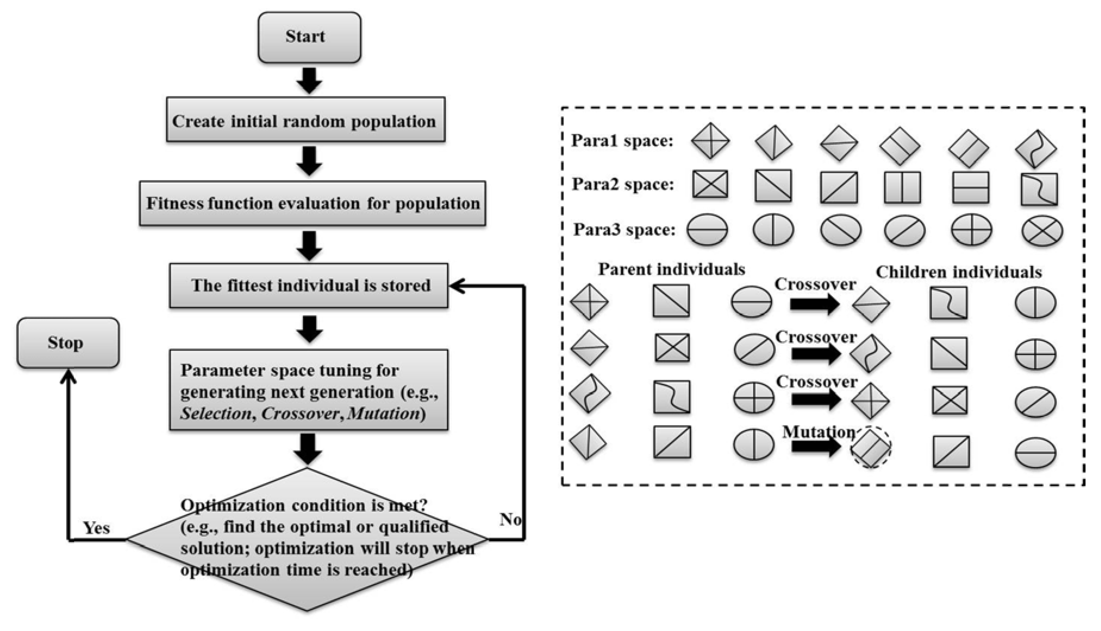
2.1. Introduction of GA

Genetic Algorithms (GAs) are stochastic search engines that mimic natural selection and biological evolution processes. Initially, a population holds randomly selected individuals that are generated from the candidate solution space. Following this, these individuals are made to evolve towards an optimal solution over successive generations via selection, crossover, and mutation processes. For GAs, the fittest individuals are selected to generate a new population of individuals at each step in the hope of improving the solution quality [19]. Figure 1 shows a brief flowchart of GAs.

Apart from GAs, several other optimization algorithms are also widely used, such as gradient-based local optimization, random search, stochastic hill climbing, simulated annealing, and symbolic artificial intelligence [20]. However, when compared with these conventional optimization methods, GAs are considered to be highly efficient techniques and distinguish themselves from traditional approaches, since their research is based on a whole population of individuals in parallel calculations rather than a single point, which improves the chance of achieving the global optimum solution and helps to avoid local stationary points. Further, the use of a fitness function (rather than derivatives) for evaluation can extend GAs to any kind of continuous or discrete optimization problems. As a domain-independent search technique, GAs are ideal for applications where domain knowledge and derivative information are difficult or impossible to provide [21]. In other words, tedious and knowledge-based processes can be greatly reduced, which is of special interest for inexperienced designers, as only the fitness function and corresponding fitness levels influence the whole search process [22,23]. Finally, some advantages of GAs are summarized and listed in Table 1.

Figure 1. Brief flowchart of genetic algorithm.

Figure 1. Brief flowchart of genetic algorithm.

Table 1. Advantages of Genetic Algorithms (GAs) when compared to conventional methods.

Advantages of GAs
√ Parallelism, efficiency, reliability, easily modified for different problems
√ Large and wide solution space searching ability
√ Non-knowledge based optimization process
√ Use of fitness function for evaluation
√ Easy to discover global optimum, avoid trapping in local optima
√ Capable of multi-objective optimization and can return a suite of potential solutions
√ Good choice for large-scale/wide variety optimization problems

Table 1. Advantages of Genetic Algorithms (GAs) when compared to conventional methods.

Advantages of GAs
√ Parallelism, efficiency, reliability, easily modified for different problems
√ Large and wide solution space searching ability
√ Non-knowledge based optimization process
√ Use of fitness function for evaluation
√ Easy to discover global optimum, avoid trapping in local optima
√ Capable of multi-objective optimization and can return a suite of potential solutions
√ Good choice for large-scale/wide variety optimization problems

2.2. GA-Based Optimization in WSNs

Genetic algorithms have been applied and to solve many engineering problems with GAs’ excellent search abilities, and the use of GAs in wireless sensor network design has been proved to be successful by a number of works. The most common use of GAs is how to achieve an energy-aware network under specific routing conditions, which includes the finding of proper cluster heads for data aggregation in the network; the selection of the optimal path to reduce hops (and thus transmission energy); and at the same time the reduction of channel contention. Such efforts for energy-efficiency can be found in [24,25,26]. In addition, researchers in [27] employed GAs in the multiple QoS (quality of service) parameter problem trying to determine near-optimal multicast routes for Mobile ad hoc network (MANET).

In [28], a GA-based methodology is proposed for adaptive wireless sensor network design. A fitness function that incorporates seven design parameters from the aspects of the specific application, network connectivity and energy consumption is used for the evaluation, so that during the optimization process many requirements (such as the status of the sensor nodes, the selection of the cluster heads, as well as the distance between nodes) are taken into account for the design of a reliable and energy-aware wireless sensor network.

In recent years, the use of GAs to find the optimal placement of wireless sensor network nodes before real deployment has gained wide attention from many research groups and academic institutions. However, in the placement problem, the optimization process is required to tune multiple conflicting objectives, e.g., reducing the energy consumption while achieving large coverage and robust connectivity, so Multi-Objective Genetic Algorithms (MOGA) are adopted in [29,30,31], aiming to find a deployed network arrangement to maximize area coverage, minimize energy cost (maximize lifetime), and maintain good connectivity.

The remainder of the paper is organized as follows. Section 3 presents the motivation of proposing the optimization framework. Section 4 illustrates the detailed design method and implementation of the proposed framework including the description of the architecture, related performance metrics, weighted sum cost function based optimization, multi-scenario/multi-objective based optimization, the settings of the framework via command lines, and a MATLAB based GUI as well as the generic use of the framework. Section 5 is the experiment part used to verify the effectiveness and availability of the framework. Finally, we conclude in Section 6.

3. Motivation of Proposing the Optimization Framework

While previous optimization efforts on hardware have been mentioned, the limited energy supply, low processing ability, low data rate, and short communication range inevitably affect the performance behavior of the whole network and also limit their further potential utilizations. The solving of these hardware-based issues to improve performance quality takes some time, such that it is difficult to satisfy rapidly evolving applications and requirements. In comparison, efforts on non-hardware (software) aspects (for instance the development of energy-efficient and robust protocols, the design of specific communication strategies or the exploration of configurations on existing protocols) can provide a quick alternative for performance optimization on given scenarios in terms of various metrics (Section 4.2).

The widely accepted methods of evaluating the above solutions before real deployment can be done through software modeling (theoretical model and simulation) or real-world testbed experiments. The latter are very time-consuming, with repeated experiments and large amounts of raw data required for subsequent evaluation, while the use of simulations/theoretical models can provide a more efficient way. When compared with simulations, theoretical models are faster to evaluate but are also sometimes idealized and inaccurate for realistic conditions. Therefore, simulation is considered to be a more suitable trade-off between accuracy and efficiency. Nevertheless, in order to get a satisfactory performance for the given scenario, the selection of the optimal WSN infrastructure, out of hundreds of potential solutions, is still required before real deployment. Thus, the use of full and exhaustive simulations to explore all possible solutions is also regarded as a very time-consuming and inefficient method.

Thus, how to effectively and accurately achieve an optimized simulation result from a large solution space is a challenge. As a fast and efficient search engine, the use of GA gives a solution. However, almost all GA-based optimization applications in wireless sensor networks mentioned in Section 2.2 are based on theoretical and analytical models. In addition to the issues of inaccuracy for realistic situations, such models always require expert knowledge in related domains as well as strong mathematical background. Therefore, it prevents many non-expert researchers and some ordinary users, without much knowledge about sensor networks, from quickly accessing the optimization process. Thus, in order to reduce time spent on evaluating all possible solutions and avoiding expert knowledge based analysis process. A generic optimization framework is proposed and will be described in detail in the following sections.

4. Design and Implementation of the Optimization Framework

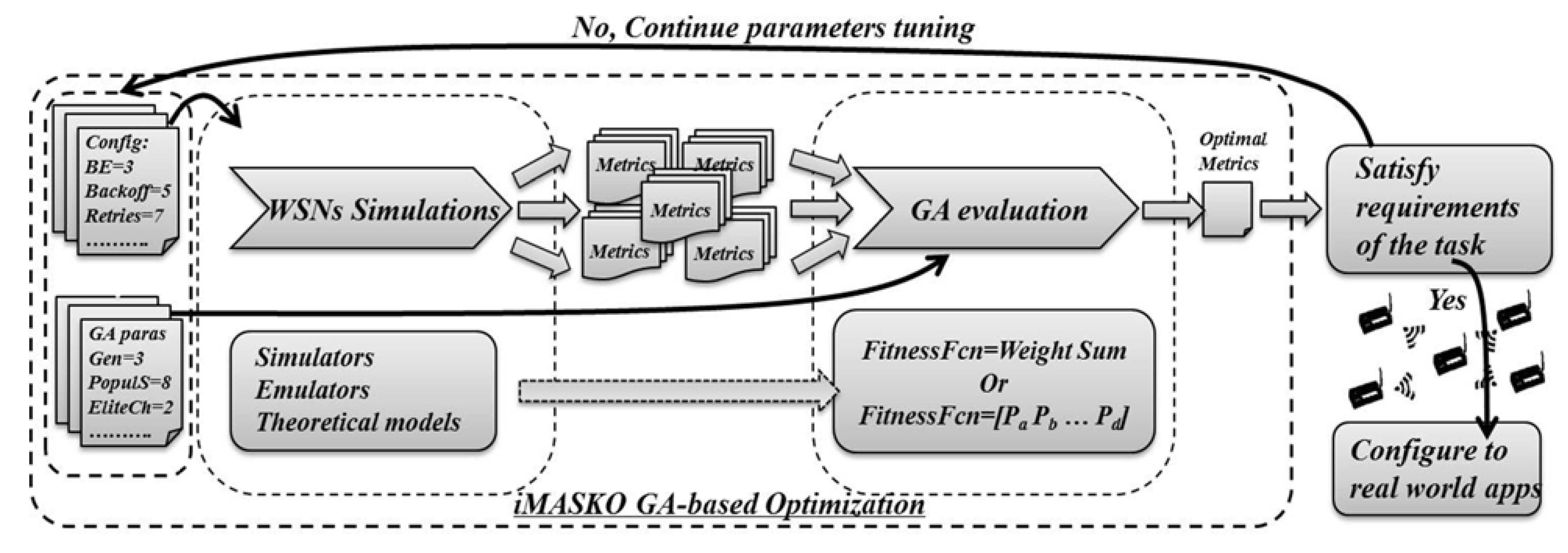
4.1. Architecture of the Framework (iMASKO)

In this section, a generic GA-based optimization framework called iMASKO (iNL@MATLAB GA-based Sensor NetworK Optimizer) is proposed. It is able to quickly and efficiently explore simulation-based results or the theoretical model-based results. Note that in this context, iMASKO is applied to automatically fine-tune the results from our house-built SystemC-based simulation [32,33,34]. In practical use, the optimization of related parameters in the design space can help find the application-specific solution to achieve the most optimal network performance for the given scenario before real deployment. By using iMASKO, only two things are needed: (i) a set of input parameters in the design space, and (ii) a user defined fitness function. As long as the system/model under evaluation can return the required data metrics to the fitness function, the detailed implementation of the system/model (simulators/emulators/mathematical models) can be ignored, which is of special interest for non-experts in wireless sensor network design. Finally, the configuration of the GA optimization process is very simple in iMASKO for users, since the interfaces of the corresponding algorithm parameters are provided and the configurations can be done via command lines and a MATLAB-based GUI.

Firstly, a brief workflow of iMASKO is presented in Figure 2 and the detailed optimization process of iMASKO is given in Table 2. Before starting the optimization, relevant parameters are fed to the simulation environment and to the GA evaluation engine respectively. Once the corresponding metrics have been generated from simulations and processed within the fitness function, the GA evaluation engine will decide whether the final result can satisfy the criteria of the given task. If so, the solution can be considered and applied in real applications. Otherwise, another cycle of the parameter tuning will start until the qualified solution for the task is found.

Figure 2. Workflow of iMASKO.

Figure 2. Workflow of iMASKO.

Table 2. Pseudo code of iNL@MATLAB GA-based Sensor NetworK Optimizer (iMASKO) optimization process.

iMASKO Optimization Process
Input initial solution: X, P ## X-parameters space, P-performance space
1: assume that: Xbest ← X, Pbest ← P
## Starting optimization until condition met
2: while stop condition not met then do #condition (e.g., max generation exceeded)
3: Xnext ← generate(X) #GA operations: selection, crossover, mutation
## Evaluations are proceeded in parallel
4: Pnext ← evaluate(Xnext) #evaluate results from SystemC simulations
5: △cost ← compare(Pnext, P) #△cost = Pnext − P
5: if△cost ≤ 0
6: X ← Xnext, P ← Pnext
7: if (P ≤Pbest)
8: Xbest ← X, Pbest ← P
9: end if
10: end if
11: end while ## when condition is met
12: return/output: Xbest, Pbest

*Note: Process 5 is not necessary, when considering the case in Section 5.1, where one population size is used.

Table 2. Pseudo code of iNL@MATLAB GA-based Sensor NetworK Optimizer (iMASKO) optimization process.

iMASKO Optimization Process
Input initial solution: X, P ## X-parameters space, P-performance space
1: assume that: Xbest ← X, Pbest ← P
## Starting optimization until condition met
2: while stop condition not met then do #condition (e.g., max generation exceeded)
3: Xnext ← generate(X) #GA operations: selection, crossover, mutation
## Evaluations are proceeded in parallel
4: Pnext ← evaluate(Xnext) #evaluate results from SystemC simulations
5: △cost ← compare(Pnext, P) #△cost = Pnext − P
5: if△cost ≤ 0
6: X ← Xnext, P ← Pnext
7: if (P ≤Pbest)
8: Xbest ← X, Pbest ← P
9: end if
10: end if
11: end while ## when condition is met
12: return/output: Xbest, Pbest

*Note: Process 5 is not necessary, when considering the case in Section 5.1, where one population size is used.

In Table 2, the typical steps of optimization are given by easily identified syntax: generate, evaluate and compare. The parameter space X could be a set of communication strategies/protocols, different configurations of a given protocol, or different application scenarios as long as the parameters that under the investigation can be represented as the qualified individuals in GAs. For the performance space P, it contains the metrics that can reflect network performance presented in Section 4.2. The metrics are returned by the fitness function in two ways: one is to combine all related metrics into a weighted sum (Section 4.3), while another is to return separated and independent metrics for multiobjective optimization problems (Section 4.4).

4.2. Performance Metrics

Despite the widespread use of wireless sensor networks and the variability in various application-specific requirements, the performance metrics that reflect the most fundamental characteristics of wireless sensor networks have always been the same, and can be classified into three major aspects: energy consumption, network reliability, and network delay.

• Energy Consumption: in most application scenarios, the sensor network must run for a long period of time to fulfill the given task without human interference (e.g., for battery recharge), thus, energy saving has always been a significant concern for extending the lifetime of the sensor network/node. Otherwise, the network will not remain operational until the required task is completed. As the energy consumption of the microcontroller (μCEnergy) and transceiver (TraEnergy) are the most power consuming parts, most works focus on saving the energy from these two parts at both the hardware and software levels. In hardware, ultra low power devices are used, especially in medical/health-care applications [2,35,36]. In software, as mentioned in Section 1, various kinds of energy-efficient MAC protocols, duty-cycling based communication strategies and data aggregation routings are proposed and measured. All kinds of efforts are made to achieve an energy-aware sensor network, and according to different requirements, energy performance could be measured and expressed in many ways (e.g., power consumption-mW, µW, lifetime-days, months, years). A taxonomy of energy related performance metrics is summarized in [37].
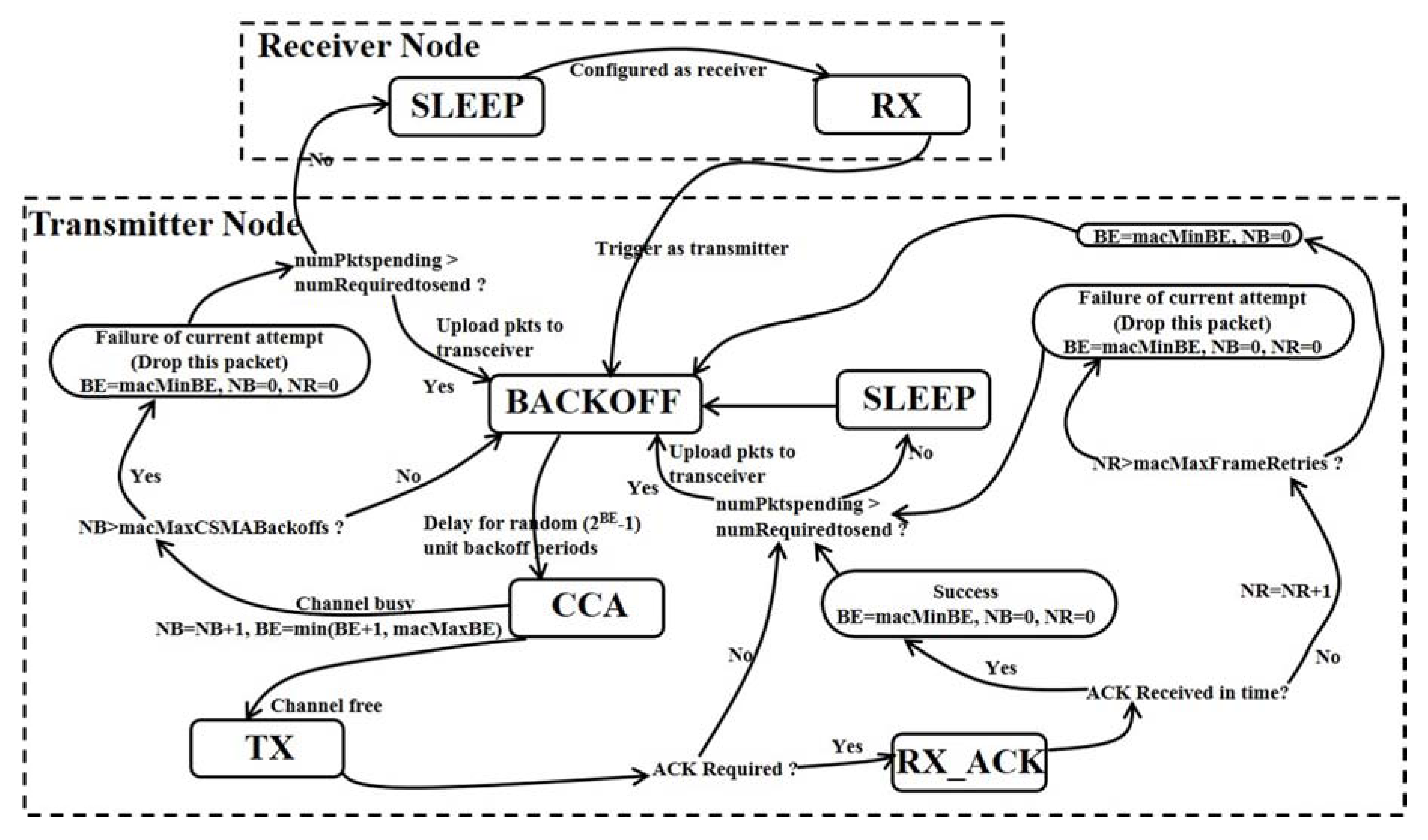
• Network Reliability: for this metric, packet loss probability (PktLossPro) or packet delivery rate (PDR) are often adopted as the evaluation standard. PDR here is defined as the ratio of the number of packets successfully received (successful receiving of ACK) to the total number of packets that are sensed for transmitting. PktLossPro is the probability that a packet sensed for sending will be dropped or fail to be transmitted (PktLossPro=1 − PDR). If a MAC layer algorithm is used, such as the unslotted/slotted CSMA/CA algorithm of IEEE 802.15.4, the packet loss can take place due to the packet drop in channel access failures (PktCAFs) and collision failures (PktCFs). PktCAFs denotes that a packet encounters (1 + macMaxCSMABackoffs) consecutive CCA failures, while PktCFs occurs when it suffers (1 + macMaxFrameBackoffs) times of collision failures, which take place during the packet transmission or transmission of the ACK frame. Besides, the loss of packet can also be caused by packet overflow (PktOverflw), which means that before starting to transmit the pending data packet (pending in MCU), a new data packet is sensed and replaces the pending packet. Therefore, evaluations can be made in detail with PktCAFs, PktCFs, and PktOverflw in addition to PktLossPro and PDR.
• Network Delay: packet latency is usually used to evaluate network delay. Packet latency can be divided into three sub-types: successful packet latency (SucPktLatency), all packet latency (AllPktLatency), and data packet latency (DataPktLatency). SucPktLatency is defined as the time interval between the instant at which the data packet is sensed and the instant at which is successfully transmitted by receiving its ACK frame. Compared to SucPktLatency, AllPktLatency takes both successful packet transmission and failure packet transmission (caused by PktCAFs or PktCFs) into consideration. DataPktLatency is calculated as the time interval from sensing the data packet to the receipt of this packet by the sink node (or coordinator).

To sum up, the fundamental features of varying WSNs applications can be evaluated from the above three major aspects, and the detailed performance metrics presented in each of the three major aspects can be used simultaneously to provide a more comprehensive insight for the given scenario.

4.3. Cost Function (Weighted Sum)

As the metrics listed above, the performance evaluation of the specific application scenario is an overall and comprehensive process which must consider multiple objectives at the same time. The evaluation engine of iMASKO returns a set of performance metrics p (Section 4.2) that need to be optimized/improved simultaneously and is given as:

(1)

where X is the parameter space. However, the solutions that can simultaneously optimize every metric are difficult to find for such a multi-objective problem. Therefore, a commonly used trade-off method combines different objectives into a linear cost function presented as a weighted sum:

(2)

where w_i is the weight vector that is designed to emphasize the importance of each performance metrics p_i. X is the parameter space, which can consist of different types of design parameters for the sensor network as shown in [28], or it can be just a set of protocol configurations if only the communication protocol is under investigation.

Thus, the multi-objective problem becomes single objective and the optimization can proceed by directly evaluating the value of the cost function. Note that this cost function in GA-based optimization is also known as the fitness function. Based on the application-specific requirements at hand, the designers can decide whether to choose all or only part of the most competing performance metrics for the fitness function. An example of a fitness function in terms of energy consumption, network reliability, and network delay can be presented as follows:

(3)

However, even with the same importance on each metric, each contribution to the weighted sum could also be different, since the scale of each metric is not the same. Hence, percentage data values are preferred to be used to reduce the impacts caused by the metrics’ scale. The above formula is thus modified as:

(4)

where nodeConsumedEnergy denotes the average energy consumption on every sensor node. TotalEnergy represents the maximum energy volume that can be used on each node. Other metrics are self-explanatory and some of them have been defined in the Section 4.2.

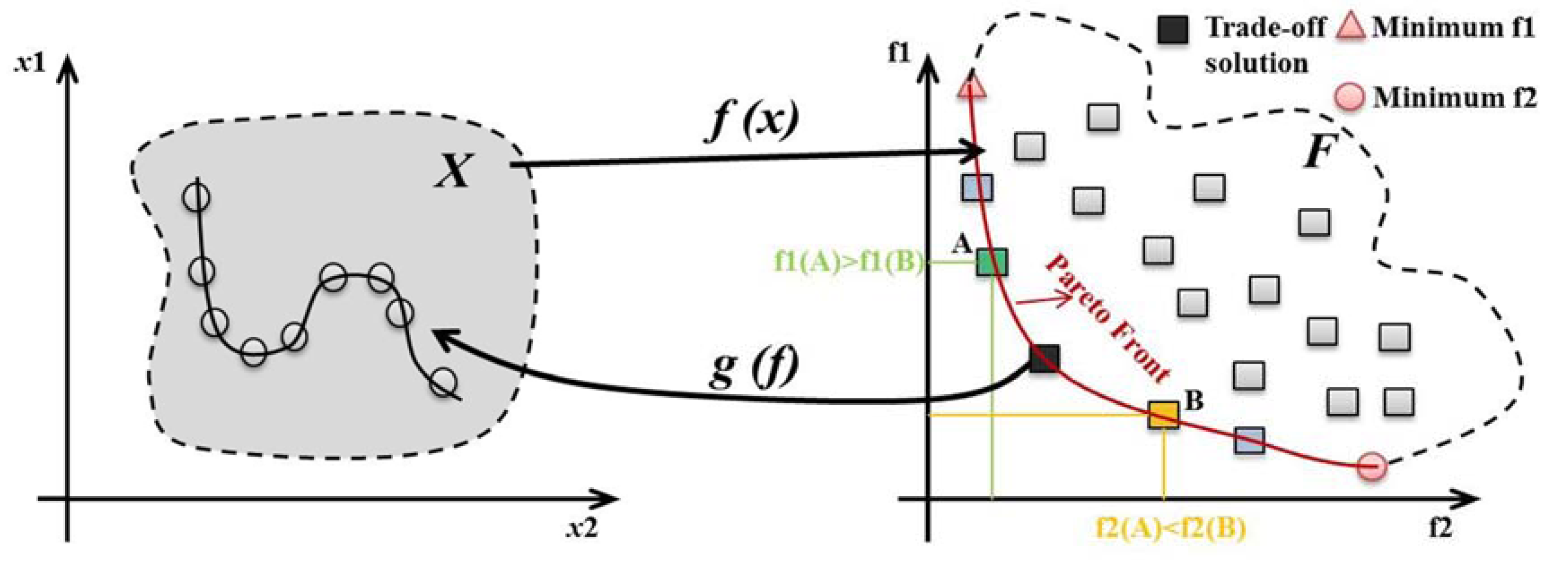
4.4. Multiobjective GA for Pareto-Front Optimization

Despite the fact that the evaluation by a weighted sum cost function facilitates the optimization process to a great extent, the most significant limitation of this process is that the metrics (e.g., energy consumption-mJ, latency-ms, packet loss-how many) used in the cost function formula are sometimes not in the same scale. Even with the use of probability values in the experimental part, the equality of scale and avoidance of implicit weighting cannot be strictly guaranteed, considering that if the given energy volume for each node is set to be a large value (e.g., 10,000 mJ) or that if a high maximum latency is used as the dividend, then the importance of energy and latency impacts will be reduced.

A more suitable solution to consider trade-offs among different metrics is Pareto-front based multi-objective optimization. As mentioned previously in Section 4.3, simultaneous multi-objective (Equation (1)) based techniques rarely exist in conventional optimization methods. However, the GA based multi-objective optimization provides an alternative, since the parallelizable characteristics of GA (represented by the population size) can help evaluate many different sets of solutions in the parameter space simultaneously, which greatly improves the efficiency. The selection of the best individuals is based on the Pareto-front (∂F , F-solution space), which can be described as a solution f = [f₁…f_n] dominating . This condition is true if each parameter of f is not greater than the corresponding parameter in f^* and there is at least one parameter that is less, i.e., for each i and for some i. This is presented as to mean f dominates f^*, and the total description in mathematics can be given as follows:

(5)

In other words, the Pareto-front is part of the boundary of performance space. On this boundary, no solution is better in criteria that makes at least one performance metric better without making other metrics worse. The Pareto front captures the trade-offs between competing performance metrics and identifies the solutions that are non-dominated, as shown in above Figure 3.

Figure 3. Pareto-front optimality.

Figure 3. Pareto-front optimality.

In addition, with design problems becoming more complex and the system under investigation integrating multiple functionalities, performance metrics of several different cases need to be evaluated at the same time. This cannot be achieved if multi-objective optimization only focuses on a specific condition. Therefore, a multi-scenario optimization method is proposed and already has applications in many engineering problems such as [22,38]. The use of this multi-scenario based multi-objective optimization is to find a robust solution which can give the optimal performance for all possible case scenarios and it can be presented as:

(6)

where X is the vector of design parameters, and p denotes a set of related performance metrics of several scenarios which are returned by iMASKO evaluation engine from the simulations.

Take two primary objectives, energy and reliability (packet loss), as the example in the optimization of network performance. If these two metrics need to be evaluated under different scenarios before practical use, the following four-dimensional (4D) front in above Figure 4 is able to transpose the concept for the case of multiple scenarios and help explore trade-offs for the metrics.

Figure 4. 4D plot for multi-objective based multi-scenario optimization [39].

Figure 4. 4D plot for multi-objective based multi-scenario optimization [39].

In this 4D coordinate, the dotted lines are plotted in quadrant one and four are the Pareto fronts. The rectangles are signs of metrics balance for different scenario requirements according to the decision maker. In this 4D Pareto front, A_Metric2 and B_Metric1 axes are reversed to make the plot clearer, and quadrant two and three are used as the auxiliary quadrant to help locate the rectangle tradeoff markers.

4.5. iMASKO Options via Command Lines and GUI

iMASKO provides a series of interfaces to configure the optimization/evaluation process by command lines, which are shown in Italics and bold letters in this section. iMASKO command line options consist of five parts which are platform selection, simulation parameter configuration, GA configuration, seed generator, and result saving respectively.

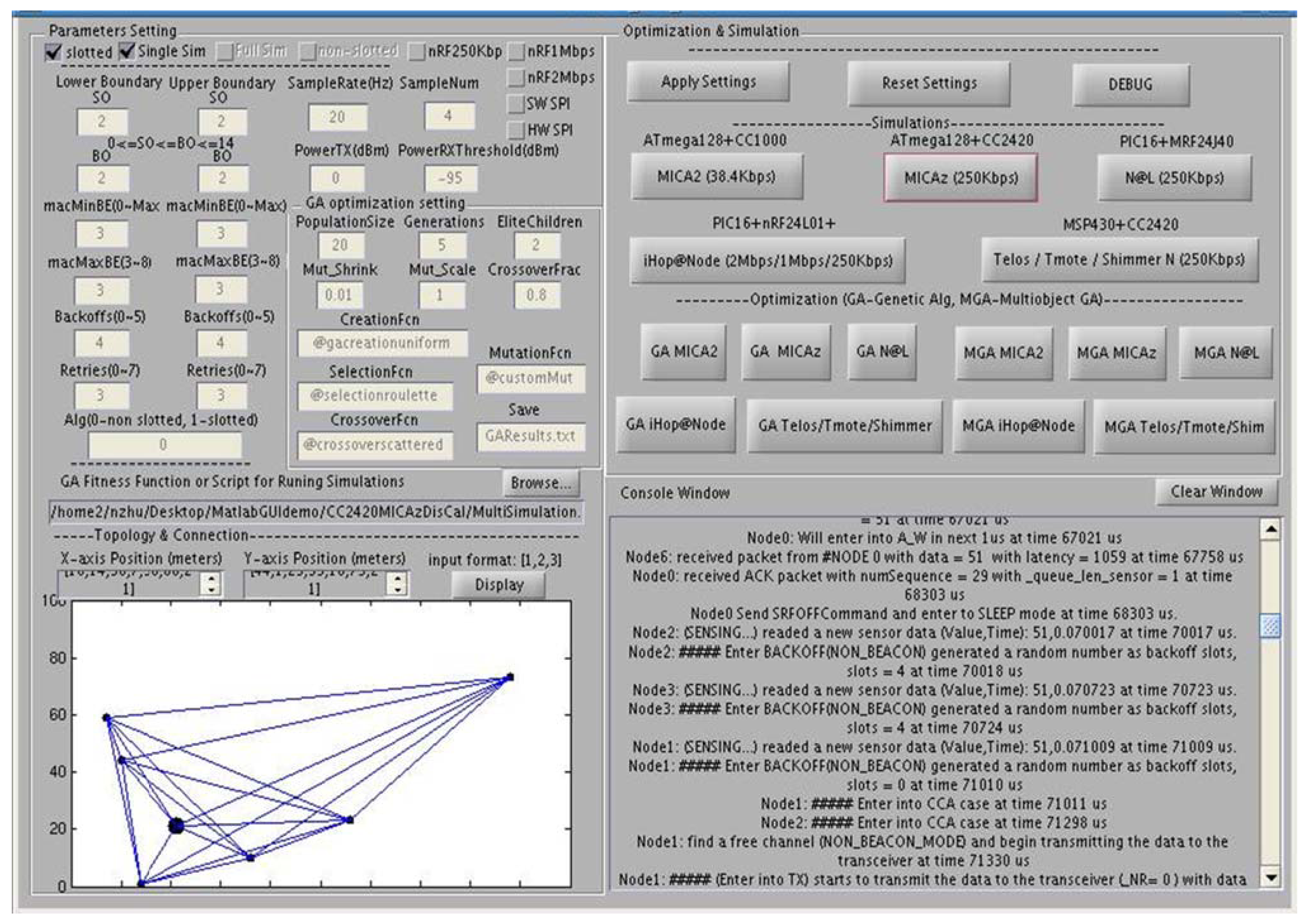
• Platform selection: this part is to load the mote platforms. Executable files of SystemC simulation are placed under the same folder, which contains several mote platforms implemented in our SystemC simulation environment (including iHop@Node [40], Telos [41], MICAz, MICA2). The option -n <platform> is adopted to select the specific mote platform for the optimization experiments. An example command line can be given as: > ./imasko -n Telos.
• Simulation parameters config: this part is used to set the corresponding parameters of SystemC simulation, such as sample rate, sample times, CSMA/CA algorithm, output power, receiver sensitivity, and independent simulation run times. The corresponding options in iMASKO for the above parameter settings are -sr <samplerate>, -st <simulationtimes>, -alg <algorithm>, -op <outputpwr>, -rs <sensitivity> and -r <runs>. Among the options, samplerate, simulationtimes, algorithm (0-unslotted, 1-slotted), outputpwr, sensitivity, and runs are all integers. An example command line would be: > ./imasko -sr 10 -st 100 -alg 0 -op 0 -rs -95 -r 50, which means that the sample rate is set as 10 Hz, the simulation runs for 100 ms, unslotted CSMA/CA is selected, output power is set as 0 dBm, receiver sensitivity is configured as −95 dBm and finally 50 independent simulations (different seeds) are required for average results. Default values will be used if the corresponding parameters are not set in the command line.
• GA config: GA related parameters are configured in this part. Parameter space under GA optimization can be configured by setting their upper and lower boundaries. In the experiment of this work, the options -lbminBE <minBElb>, -ubminBE <minBEub>, -lbmaxBE <maxBElb>, -ubmaxBE <maxBEub>, -lbBackoff <Backofflb>, -ubBackoff<Backoffub>, -lbRetries<Retrieslb> and -ubRetries<Retriesub> are used to specify the lower and upper bounds of the unslotted algorithm’s four parameters, which are macMinBE, macMaxBE, macMaxCSMABackoffs and macMaxFrameRetries. These boundary values are used to limit the parameter space range during the whole optimization process, and they can also be employed to initialize the PopInitRange parameter in GA at the very beginning of the optimization. In addition, other commonly used GA parameters are also configurable by command lines, the provided parameters include GA’s PopulationSize, Generations, CrossoverFraction, CreationFcn, SelectionFcn, MutationFcn, CrossoverFcn. The corresponding options in iMASKO are -ps <populationsize>, -g <generations>, -cf <crossoverfraction>, -creatf <@creationfunction>, -selectf <@selectionfunction>, -mutf <@mutationfunction>, and -crossf <@crossoverfunction>. Among these options, populationsize and generations are integers, crossoverfraction is a float number within the range 0 through 1. Finally, creationfunction, selectionfunction, mutationfunction, and crossoverfunction are the names of the functions which are provided by the GA library (e.g., @gacreationuniform, @selectionstochunif, @mutationgaussian, @crossoverscattered) or the user custom functions. Likewise, if the parameters are not set via the command line, default values will be used. An example command line can be: > ./imasko -ps 20 -g 100 -cf 0.8 -mutf @mutationgaussian.
• Seeds Generator: due to the quad-core CPUs of the server, each simulation actually consists of four parallel and independent (independent seeds) runs for average results, so the use of -s1 <seeds1>, -s2 <seeds2>, -s3 <seeds3> and -s4 <seeds5> (integers for seeds1, seeds2, seeds3, and seeds4) can specify different seeds for the four independent runs, and all the generated seeds can be stored and used in the optimization process to guarantee reproducibility of results
• Result Saving: the use of -save <filename> can save the final result file with the user defined file name and with any suffix. As an example: > ./imasko -save GAresults.log.

As the requirements of different tasks are application-specific and vary all the time, the complete configuration of iMASKO options via command lines not only satisfies the varying requirements, but also provides a flexible and effective way to set related parameters in the optimization/evaluation process for the given scenario.

Since iMASKO command line options are not intuitive especially for non-experience designers and users, a MATLAB based GUI has been developed to link simulation and optimization, which facilitates configurations on both sides and makes the evaluation process visualizable. The GUI is shown in Figure 5, where all parameters mentioned in the previous section can be set in the corresponding edit box. Default values are used if the parameters are not set. All these parameters are passed to the simulation and GA evaluation engine by pressing the “Apply” button, and the evaluation will start when a specific platform is chosen on the right side of the GUI.

Figure 5. iMASKO GUI.

Figure 5. iMASKO GUI.

4.6. Generic Use of iMASKO

Except for the multiple and detailed configuration interfaces support, iMASKO is generic in its use of the optimization/evaluation process. In this work, the fitness function uses iWEEP’s SystemC-based simulation results. However, the fitness function in iMASKO can be of multiple types as long as it provides parameter space inputs and performance metrics outputs. Thus, results from other well-known WSN simulators, such as NS-2, OMNeT++ [42] and Prowler [43], can also be used under the evaluation of iMASKO, even if the detailed implementation and knowledge of such simulations are unknown. For instance, an executable C++ file of NS-2 and OMNeT++, as well as MATLAB’s m-file of Prowler, are all able to act as the fitness function, since the required performance metrics in the fitness function can be generated after the execution of these files. In addition, in some cases if the simulation process is controlled by a shell script, then such a shell script represents the fitness function. Furthermore, if the simulation is implemented directly in MATLAB as a theoretical model, then this m-file function can be used as the fitness function. Therefore, iMASKO GUI provides for path loading to help select different types of fitness functions (in the mid-left of GUI) according to each specific case.

5. Experimental Results

In this experimental results section, the optimization framework is verified by using two test cases in Section 5.1 and Section 5.2. The test cases are carefully chosen to prove the framework’s ability to search quickly for optimal performances, as well as its capability for fine tuning the parameter space in wireless sensor networks. For this work, the optimization process is based on the tuning of parameter configurations of existing protocols to achieve the best optimal behavior. In both cases, the parameter space under investigation consists of the four parameters of the unslotted CSMA/CA algorithm [17], which are macMinBE, macMaxBE, macMaxCSMABackoffs, and macMaxFrameRetries. With the range from 3 to 8 for macMaxBE, 0 to macMaxBE for macMinBE, 0 to 5 for macMaxCSMABackoffs, and 0 to 8 for macMaxFrameRetries, the total number of solutions has a wide possibility of 1,872 combinations in the parameter space. Figure 6 shows the flowchart of the unslotted CSMA/CA algorithm.

As shown in Figure 6, the transmitter node first performs a random backoff duration and checks the channel status. If the channel is detected to be busy, and the number of CCA attempts is larger than the protocol parameter macMaxCSMABackoffs, then a Channel Access Failure (CAF) is reported. If, on the other hand, the number of CCA attempts is smaller than macMaxCSMABackoffs, the transmitter node will go back for a new round of random backoff process. When the channel is indicated as free by CCA, the transmitter node will send a packet to its transceiver and trigger over-the-air transmission. After the transmission of an ACK required data packet, the protocol will make the transmitter node wait within a fixed time period (0.864 ms or 54 symbols) for the ACK frame confirmation. If ACK is received in time, this transmission is regarded as successful. Otherwise, the packet retransmission process will start. A Collision Failure (CF) occurs only after failure to receive ACK frame macMaxFrameRetries times, which might be caused by collision of data packets or collision between data packets and the ACK frames. In addition, as long as there are pending data packets in the node, they will be uploaded to the transceiver immediately, once the transmission process is over (no matter whether a success or a failure), which is to guarantee the timeliness and reliability of data transmission. In this work, the unslotted CSMA/CA algorithm is implemented in our SystemC-based simulation engine [32,33], and iMASKO is used to fine tune simulation’s parameter space (macMinBE, macMaxBE, macMaxCSMABackoffs, macMaxFrameRetries) for the optimum performance metrics based on the requirements of the given application.

Figure 6. Unslotted CSMA/CA algorithm model.

Figure 6. Unslotted CSMA/CA algorithm model.

In the following two sub-sections, the first case applies a weighted sum fitness function as the trade-off for evaluating multiple performance metrics. The second case is for a simultaneous multi-objective optimization under multi-scenario conditions. All the experiments performed in this section were executed on an Intel Xeon server operating with Linux CentOS (4 CPUs, 8 GB RAM, 2.4 GHz).

5.1. Part I—Results of Weighted Sum Optimization

In this part, the search efficiency and reliability of this GA-based framework is tested. The performance metrics in terms of energy consumption, packet loss and packet delay are from our SystemC-based simulation which has 30 Telos nodes, 10 Hz sampling rate, 32 bytes payload in each data packet, and 4 s of simulation time and each sensor node transmits the data to the common sink node. The three performance metrics are modeled into a linear weighted sum cost function as the trade-off optimization method, to find the best optimal performance weighted sum value via the tuning of unslotted algorithm’s parameter configuration. Finally, the GA-based optimizations are compared with the time-consuming full/exhaustive simulations (simulations on all possible solutions) in terms of efficiency and results. The weighted sum cost function is derived from (Equation (4)) and given as follows:

(7)

In this test, the same importance is given to the three metrics with each weight vector as 1. Percentage numbers are used for the performance metrics to reduce the impact of the metrics’ contribution in the weighted sum. Here, TotalEnergy is given as 250 mJ (in the experiment, the maximum energy will not exceed 250 mJ). The use of twice the sample interval is because latency could sometimes exceed 100 ms (1*Sample Interval) when longer backoff wait time happens, which can be caused by the use of larger BE value.

The GA implemented in MATLAB R2012a has been integrated in the iMASKO framework and used for the parameter tuning in the experiment. The parameters of the unslotted algorithm are all integers rather than real numbers. Although MATLAB R2012a has a built-in integer number based optimization support, it provides limited configuration options. Namely, if integer optimization is applied, many commonly used options cannot be configured, such as the settings of CreationFcn, SelectionFcn, CrossoverFcn, MutationFcn, EliteCount, and CrossoverFraction are all unavailable in integer problems according to the user guide. Therefore, the default real number optimization is used in our experiments but with custom functions like CreationFcn and MutationFcn to produce integer individual parents and integer mutation children, in which the evaluation can proceed totally based on integer optimization while at the same time all the options in GA can be configured according to the problems at designers’ hands.

In addition, the typical data sensing start point of each node is randomly generated by feeding with different seed values, but it could also be fixed with the same sensing start time. Since the different random sensing start time of the data can affect the network condition (even with the same combination of protocol parameters), the final performance results could be different. Hence, fixing the same data starting time can avoid such unpredictable elements and helps GA to effectively search the parameter space for the best performance exploration. The fixed starting point can be controlled by employing a set of fixed seeds (four different seeds are used for four parallel simulations, four runs for the average simulation result), which ensures that under each parameter combination case every node starts to generate the data at the same instant. This approach is typically used to reproduce the given result, and here enables the comparison between optimization results and exhaustive/full simulation results to validate the efficiency of GA’s searching ability under the proposed iMASKO framework.

The comparison results are shown in the following part. At first, the weighted sum results of exhaustive/full simulations are presented in Table 3. In the table, since macMinBE must be less than macMaxBE, the value of macMaxBE is fixed as the maximum value for macMinBE in each row of the table. The range of weighted sum results are given in each fixed macMaxBE case and the total simulation time is also provided.

Table 3. Exhaustive/Full simulation results.

Fixed macMaxBE	Parameter Combinations	Weight Sum Range	Simulation Time (min)
3	192	0.504349 ~ 0.812070	34.397
4	240	0.498976 ~ 0.982988	43.622
5	288	0.497637 ~ 1.292583	53.144
6	336	0.507912 ~ 1.747466	61.901
7	384	0.507912 ~ 1.834899	69.886
8	432	0.507912 ~ 1.935943	76.702
Total	1,872	0.497637 ~ 1.935943	339

Table 3. Exhaustive/Full simulation results.

Fixed macMaxBE	Parameter Combinations	Weight Sum Range	Simulation Time (min)
3	192	0.504349 ~ 0.812070	34.397
4	240	0.498976 ~ 0.982988	43.622
5	288	0.497637 ~ 1.292583	53.144
6	336	0.507912 ~ 1.747466	61.901
7	384	0.507912 ~ 1.834899	69.886
8	432	0.507912 ~ 1.935943	76.702
Total	1,872	0.497637 ~ 1.935943	339

The GA optimizations were launched with the settings of 2 elitecount, 0.8 crossoverfraction, and the roulette based selection process. A larger population size for individuals and more generations can certainly provide better optimization results, but at the cost of time. In this experiment, with the general efficiency and availability of the GA-based framework under the test, four population sizes with only one generation were measured (5/10/20/30 populationsize, 1 generation), since they were able to provide good results. Under each population size case, GA ran 100 times to determine the average results, because different seed values were generated according to the current time in every GA run. Hence, the randomly formed initial parent individuals, the children after crossover and mutation could be different, which led to different final results. Table 4 gives the efficiency information in terms of time and availability information in terms of the statistics probability of results falling into the weighted sum range area.

Table 4. Test results of GA-based optimization.

Full Weighted Sum Range:      0.497637-----------------------------------------> 1.935943
Area	0.5%	1%	2%	3%	4%	5%	6%	7%	8%
Value	0.5048	0.5120	0.5264	0.5408	0.5552	0.5696	0.5839	0.5983	0.6127
Popul Size (Opt time)	The following statistics indicate the probabilities that optimization results fall within each specific area (Average optimization time for 5/10/20/30 are shown next to the population size)
5 (1.28 min)	2%	19%	45%	74%	85%	91%	94%	97%	98%
10 (2.74 min)	3%	35%	72%	94%	100%	100%	100%	100%	100%
20 (5.25 min)	5%	63%	94%	100%	100%	100%	100%	100%	100%
30 (8.00 min)	7%	76%	99%	100%	100%	100%	100%	100%	100%

Table 4. Test results of GA-based optimization.

Full Weighted Sum Range:      0.497637-----------------------------------------> 1.935943
Area	0.5%	1%	2%	3%	4%	5%	6%	7%	8%
Value	0.5048	0.5120	0.5264	0.5408	0.5552	0.5696	0.5839	0.5983	0.6127
Popul Size (Opt time)	The following statistics indicate the probabilities that optimization results fall within each specific area (Average optimization time for 5/10/20/30 are shown next to the population size)
5 (1.28 min)	2%	19%	45%	74%	85%	91%	94%	97%	98%
10 (2.74 min)	3%	35%	72%	94%	100%	100%	100%	100%	100%
20 (5.25 min)	5%	63%	94%	100%	100%	100%	100%	100%	100%
30 (8.00 min)	7%	76%	99%	100%	100%	100%	100%	100%	100%

The results show that even with a small population size of 5, the probability of achieving cost values inside 7% of the weighted sum range area is over 95%, while the optimization time is only about 1/264 compared to the exhaustive simulation. When the population size is raised to 10, there is over a 90% probability of achieving the area, which is 3% in the weighted sum range area, while the time is about 1/123 of the exhaustive simulation. Performances are further improved when the population size reaches 20 and 30, with all the results within the 3% of the weight sum area at a small cost of optimization time, which is about 1/64 and 1/42 respectively. On the other hand, for non-expert researchers and users who do not have much knowledge in how the configuration of the unslotted algorithm can affect performances, the default configuration ([macMinBE=3, macMaxBE=5, macMaxCSMABackoffs=4, macMaxFrameRetries=3]) of the algorithm could always be the priority of their choice for the comparison. In this experiment, the default configuration weighted sum value is 0.737, so even with 5 population sized GA optimization all solutions can have better performance than this default configuration. Note that if another set of seed values are used, the above results could be different, but not significantly so, according to our tests. In addition, similar efficiency and availability can be achieved for MICAz, MICA2, iHop@Node based networks under the iMASKO framework.

On the other hand, when a larger scale scenario (e.g., 80 Telos nodes) is considered in iMASKO, firstly the optimization time will increase, because the SystemC simulation needs more time for a larger scale network scenario. Secondly, the optimization performance in this large scale scenario could be not that obvious as in the small scale scenario, which is caused by the same level range of performance metrics under most of protocol parameter configurations, and the reason is analyzed as follows: with a large number of nodes competing for the channel, an occupied channel is always expected. Based on the experimental results, most of the protocol parameter configurations applied in the large scale network give very close and stable values on energy consumption, packet loss, and packet latency. This is due to the busy channel conditions where packets are difficult to be sent and received, so packet loss keeps the same high-level range and so does for the packet latency. While for the energy consumption, the nodes tend to use up all the predefined protocol overhead (e.g., backoff duration, channel attempts, retransmission) and, hence, are more likely to maintain in active mode against the occupied channel for the data transmission. Therefore, energy consumption under most of the protocol configurations are expected to be in the same level, except for the configurations with smaller values where the protocol overhead can always be depleted before the next data transmission, so more sleep time can be acquired for the energy saving. Overall, iMASKO is capable of large scale network scenario optimization but as only a framework the optimization performance is greatly affected by the simulation/theoretical models as well as the detailed network conditions (optimization performance could be different, if 250 kbps data rate based Telos motes are replaced by 1Mbps data rate based iHop@Node in this 80 node scenario).

In addition, the computational feasibility of iMASKO for the exhaustive search of large scale scenario can be different when simulation model (model from simulator/emulator) and mathematic formula model are respectively employed. To optimize the performance metrics from simulation model, iMASKO firstly has to wait the generated metrics from the simulation run and then can proceed to the evolution process. Thus, high efficiency cannot be guaranteed when longer time is required by the simulation for the given task. However, if mathematic formula based models implemented in m-file are used, iMASKO can launch many calculations with different parameter configurations in parallel, which can greatly accelerate the whole optimization process. In summary, iMASKO is computational feasible for the exhaustive search in large scale scenario but its performance is significantly affected by the type of software model it uses (simulation/emulation model, mathematic formula model).

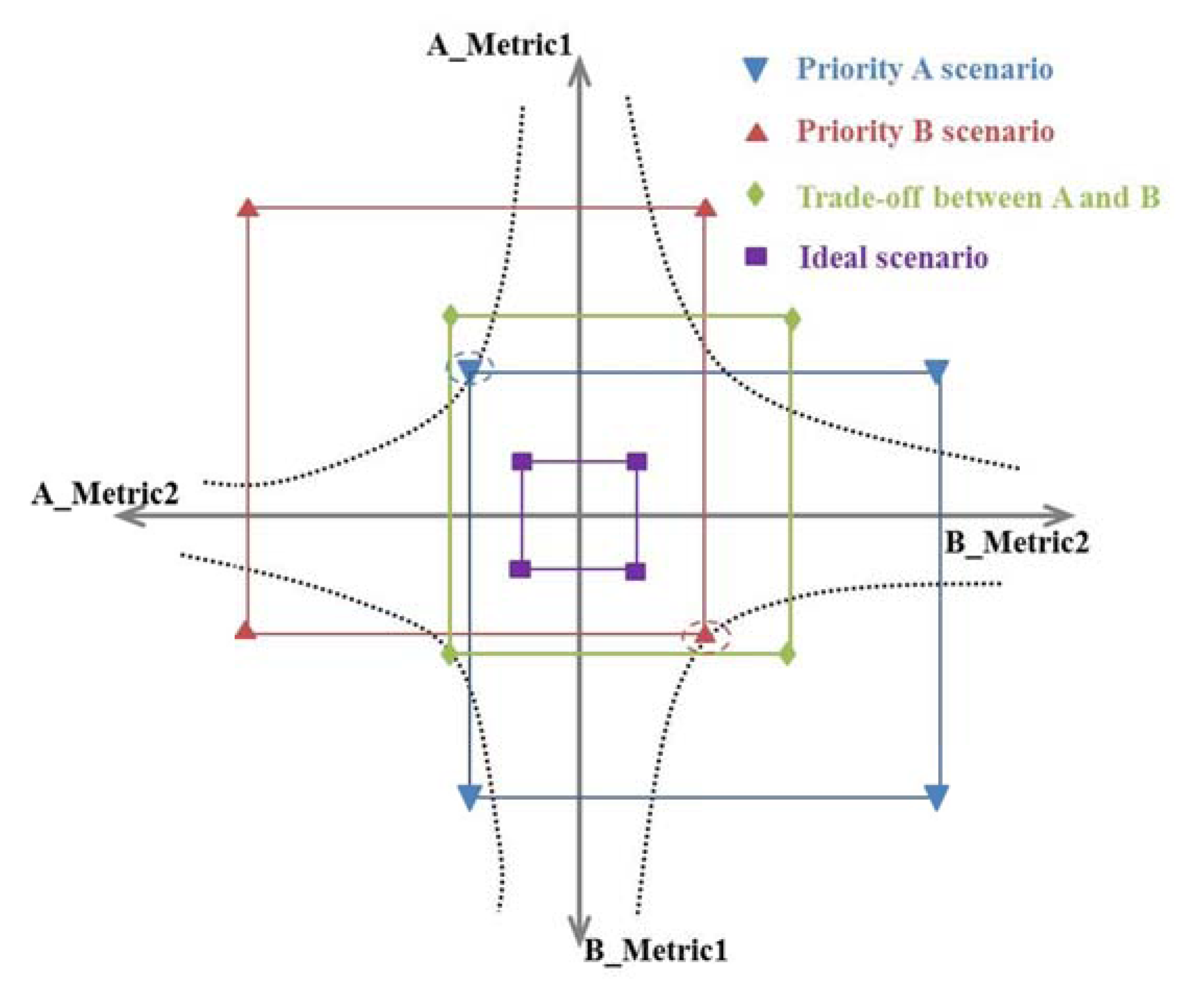
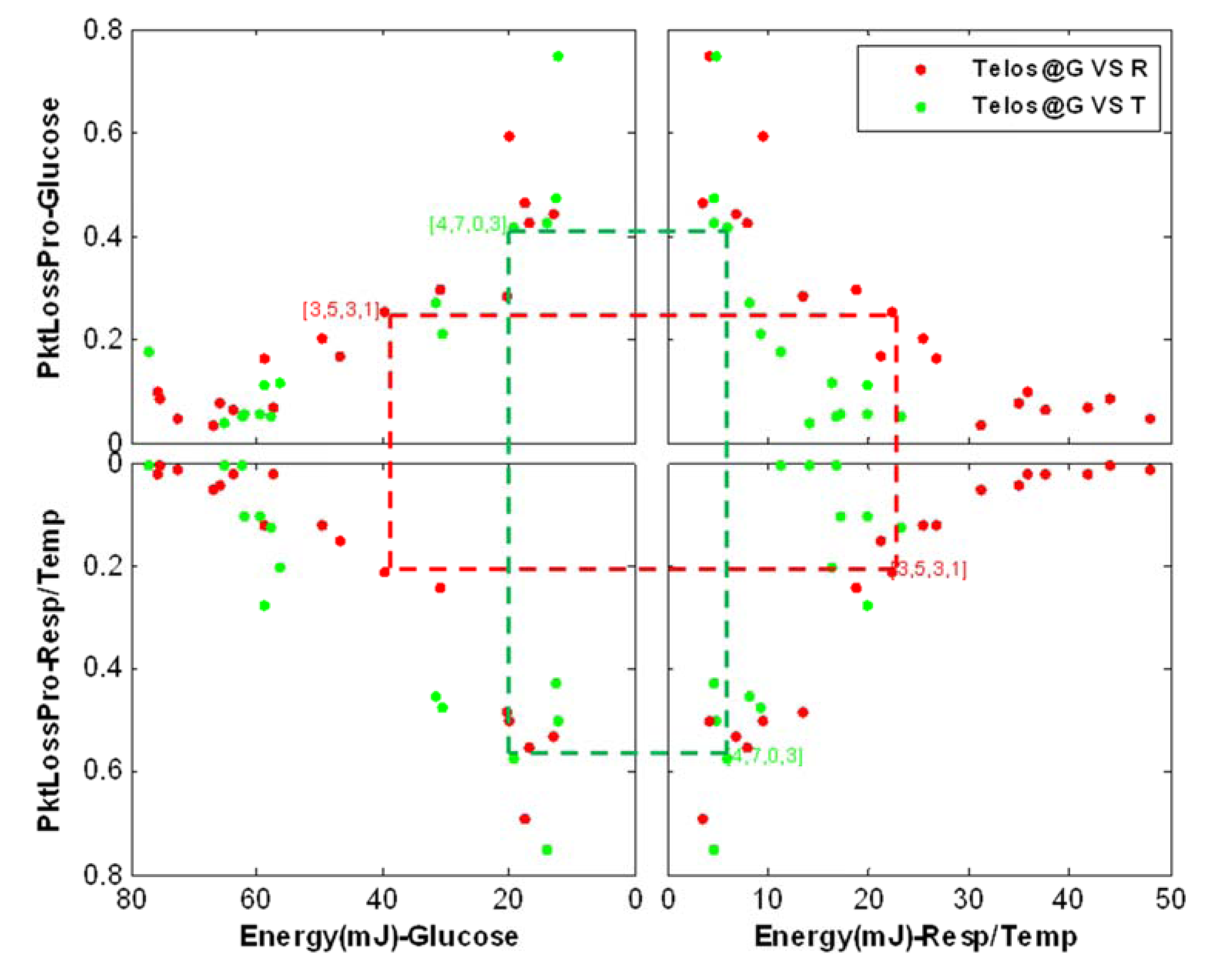
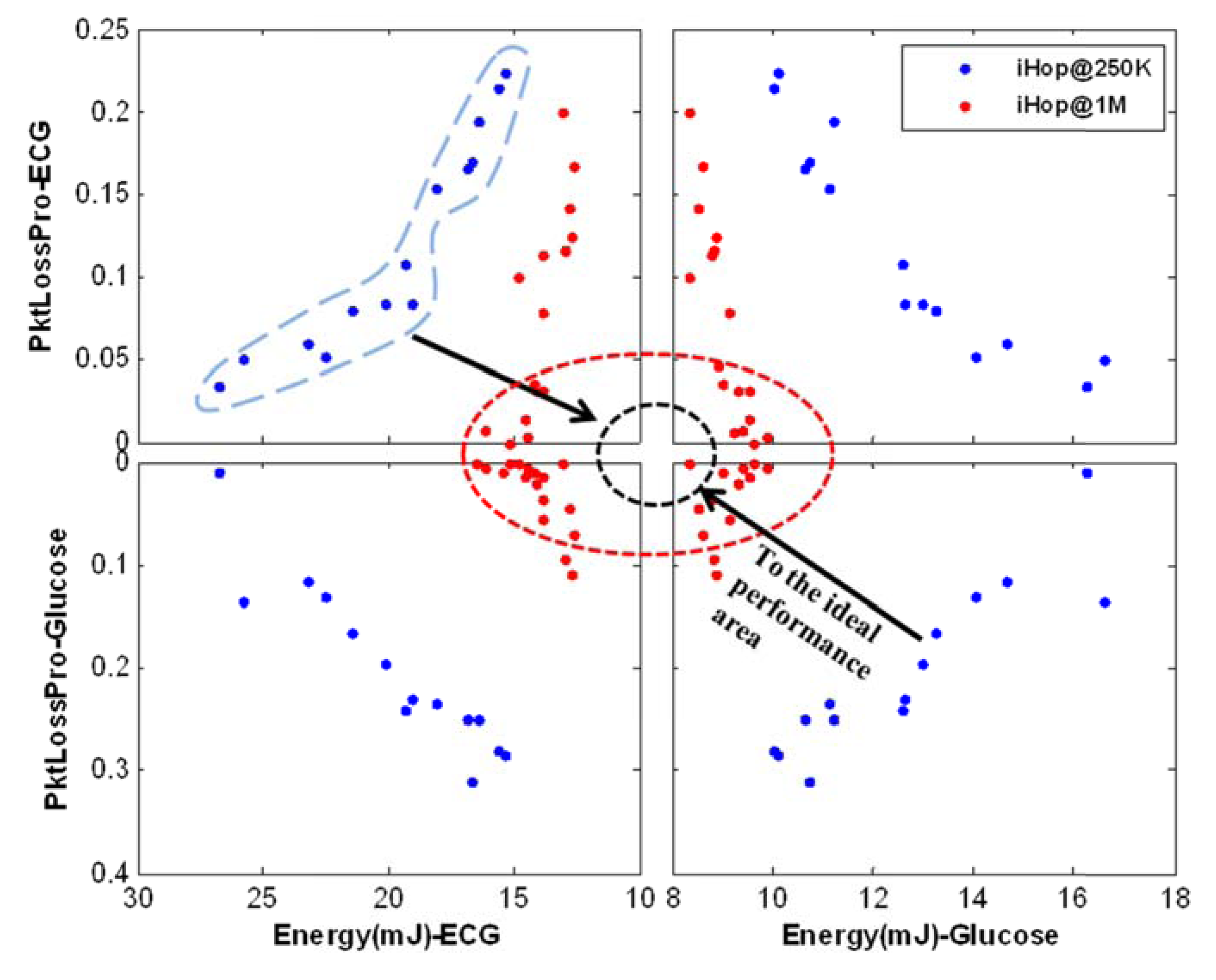
5.2. Part II—Results of Multi-Scenario and Multi-Objective Optimization

The main goal of this test case is to verify the capability of the iMASKO framework under the conditions of multi-scenario and multi-objective optimization. The case applied in this experiment is the typical wireless body area networks (WBANs) [44,45], which are widely used in medical and health care applications and it is shown in Figure 7. This typical on-body sensor network consists of six different functional sensor nodes for physiological signals monitoring and measurement, which are ECG (electrocardiogram, 125 Hz sampling rate) sensor node for measuring the rate and regularity of heartbeats, Arterial (125 Hz) and Glucose (50 Hz) nodes for pressure measurements, Motion node (100 Hz) for movement strength recording, Respiration node (25 Hz) for the test of respiration frequency, and Temperature node (10 Hz) for the real-time temperature monitoring of human body. In the experiments, both Telos node and iHop@Node [40] based networks are under investigation, the typical payload length in the packet is set to 2 bytes, and each simulation is set to 2 s. Fixed seed values are also adopted to mitigate the influence of the starting time of data sensing. Further, note that iHop@Node consists of a low power microcontroller PIC16F88 [46] and a high data rate transceiver nRF24L01+ [47] which supports the rate of 2 Mbps, 1 Mbps, and 250 kbps. Since that Microchip’s non-beacon based (unslotted CSMA/CA algorithm) MiWi [48] protocol stack is designed for PIC microcontroller families from PIC16 to dsPIC33, so the simulation of unslotted CSMA/CA algorithm is implemented in the PIC16F88 microcontroller of iHop@Node and related results will be shown (detailed use of unslotted CSMA/CA algorithm on iHop@Node is described in [1]).

Figure 7. Typical WBANs for medical and health care.

Figure 7. Typical WBANs for medical and health care.

For such a network, each sensor node represents a specific scenario, and the use of different configurations of the unslotted CSMA/CA algorithm under this multi-scenario case could cause different performances at each sensor node. Note that in this experiment during the algorithm tuning process, the same algorithm parameter combination is used to configure all sensor nodes. As mentioned previously, performance optimization problems always involve multiple objectives to be met simultaneously in each specific scenario. These objectives are usually conflicting such as achieving maximum network reliability and at the same time minimizing the energy consumption. However, this kind of situation cannot happen most of the time, because with channel competition packet loss can be prevented if more channel access attempts, retransmission attempts, or longer backoff wait time are used, and hence more energy will be consumed in these processes. Therefore, there is no single solution to a multi-objective optimization problem such as this one, in addition to the use of the Pareto front method to find a set of mathematically equal solutions (Section 4.4).

In the test, two objectives (energy consumption and packet loss rate) are subjected to optimization within the framework to achieve the solution trade-offs. In the multi-scenario situation of the network, the fitness function of each individual is composed of two pairs of energy consumption and packet loss rate for two different sensor nodes. The detailed fitness function is given as:

(8)

where X is the parameter space of the unslotted algorithm (four parameters). Node1 and Node2 are different nodes that are selected from ECG, Arterial, Motion, Glucose, Respiration, and Temperature sensor nodes. The multi-objective genetic algorithm in MATLAB R2012a optimization toolbox (ver. 6.2) was integrated into the iMASKO framework and was used to generate the Pareto front for energy consumption and packet loss probability. The GA was configured for 60 initial integer individuals, 30 generations, scattered crossover, 0.8 crossover fraction as well as 2 elite children. Figure 8 shows the obtained four-dimensional Pareto front from the Telos mote based network.

Figure 8. Energy and packet loss Pareto front (Glucose vs. Respiration/Temperature).

Figure 8. Energy and packet loss Pareto front (Glucose vs. Respiration/Temperature).

In the Figure, the node energy consumption and network packet loss rate of the glucose sensor node are compared with the corresponding performance metrics of the respiration and temperature nodes respectively. According to the problem requirements, a good tradeoff solution for both energy and reliability can be manually selected by the decision maker based on their knowledge and intuitive experience (e.g., dashed rectangle in the Figure 8). Algorithm configurations are also presented next to the tradeoff point in the Figure 8 (e.g., [macMinBE, macMaxBE, macMaxFrameBackoffs, macMaxFrameRetries] = [3, 5, 3, 1]). On the other hand, while the glucose sensor node is in both experiments, the results show that under such multi-scenario network conditions, the best tradeoff solution for two specific cases might not guarantee the best tradeoff for another two cases. Therefore, if an overall tradeoff solution is required for the whole network then a more comprehensive optimization on all possible scenarios needs to be evaluated.

In addition, the performances (energy, reliability) of the highest sample rate based ECG node are also tested and compared with the glucose node for the iHop@Node based network. Two cases were under investigation, 1 Mbps based high data rate and 250 kbps based low data rate. Figure 9 shows the 4D Pareto front between energy cost and packet loss for two data rate cases.

Figure 9. Energy and packet loss Pareto front (ECG vs. Glucose 1 Mb and 250 kb).

Figure 9. Energy and packet loss Pareto front (ECG vs. Glucose 1 Mb and 250 kb).

The results in Figure 9 show that the balance of tradeoffs between energy consumption and packet loss still needs to be found on the Pareto front for both data rate cases. As compared to the commonly used 250 kb low data rate, the high data rate based network can provide both lower energy consumption and packet loss, which brings it closer to the ideal performance area. This is because the high data rate reduces the channel occupation condition, so more packets can be successfully transmitted. For energy saving, this comes from two parts. Firstly, with good channel conditions under high data rate, mechanisms like repeated channel check and retransmission in the unslotted algorithm are no longer necessary, since almost all the packets can be successfully transmitted with one attempt, and energy is saved from protocol overhead. Secondly, despite the fact that a high data rate case consumes more current during the packet and ACK frame transmission, the time spent in both transmissions are greatly reduced due to the high data rate, and ultimately a large amount of energy can be saved from this part.

6. Conclusion and Future Work

In this work, a generic genetic algorithm-based optimization framework iMASKO is proposed for the performance metric optimization of wireless sensor networks. It supports the optimization of both theoretical analysis based models and simulation based models. The high efficiency and availability of the framework have been proved by modeling the required performance metrics into a weighted sum based cost function and comparing these results with exhaustive simulations. In the meantime, with the study of a typical health-care network on human body, the simultaneous optimization of four performance metrics on different node platforms and different data rates has proved that the framework can well support multi-scenario and multi-objective based optimization.

For the future work, in the weighted sum based optimization, how to make each metric belong to strictly the same scale is still a challenge. In addition to the simple linear weighted sum cost function for the protocol parameter optimization, a set of fundamental performance bounds is required since it is essential for determining whether the target protocol is appropriate for a specific network design choice [49]. On the other hand, the optimization of SystemC-based simulation could improve the whole evaluation process of the framework even when larger population size and generations are employed.

References

1. Zhu, N.H.; O’Connor, I. Performance Evaluations of Unslotted CSMA/CA Algorithm at High Data Rate WSNs Scenario. In Proceeding of the 9th IEEE International Wireless Communications and Mobile Computing Conference (IWCMC 2013), Cagliari, Italy, 1–5 July 2013; pp. 406–411.
2. Mackensen, E.; Lai, M.; Wendt, T.M. Bluetooth Low Energy (BLE) based wireless sensors. IEEE Sens. 2012, 1–4. [Google Scholar]
3. Zhang, J.Y.; Orlik, P.V.; Sahinoglu, Z.; Molisch, A.F.; Kinney, P. UWB systems for wireless sensor networks. Proc. IEEE 2009, 97, 313–331. [Google Scholar] [CrossRef]
4. Buratti, C.; Conti, A.; Dardari, D.; Verdone, R. An overview on wireless sensor networks technology and evolution. Sensors 2009, 9, 6869–6896. [Google Scholar] [CrossRef]
5. Castagnetti, A.; Pegatoquet, A.; Belleudy, C.; Auguin, M. A framework for modeling and simulating energy harvesting WSN nodes with efficient power management policies. EURASIP J. Embed. Sys. 2012, 8, 1–20. [Google Scholar]
6. Sonavane, S.S.; Kumar, V.; Patil, B.P. MSP430 and nRF24L01 based wireless sensor network design with adaptive power control. ICGST CNIR J. 2009, 8, 11–15. [Google Scholar]
7. Pouwelse, J.; Langendoen, K.; Sips, H. Dynamic Voltage Scaling on a Low-Power Microprocessor. In Proceeding of the 7th Annual International Conference on Mobile Computing and Networking, Rome, Italy, 16–21 July 2001; pp. 251–259.
8. Benini, L.; Bogliolo, A.; de Micheli, G. A survey of design techniques for system-level dynamic power management. IEEE Trans. Large Scale Integr. Sys. 2000, 8, 299–316. [Google Scholar] [CrossRef]
9. Ye, W.; Heidemann, J.; Estrin, D. Medium access control with coordinated adaptive sleeping for wireless sensor networks. IEEE/ACM Trans. Netw. 2004, 12, 493–506. [Google Scholar] [CrossRef]
10. van Dam, T.; Langendoen, K. An Adaptive Energy-Efficient MAC Protocol for Wireless Sensor Networks. In Proceeding of the First ACM SenSys conference, Los Angeles, CA, USA, 5–7 November 2003; pp. 171–180.
11. El-Hoiydi, A.; Decotignie, J.D.; Enz, C.; le Roux, E. WiseMAC: An Ultra Low Power MAC Protocol for the WiseNET Wireless Sensor Network. In Proceeding of the First ACM SenSys Conference (SenSys 2003), Los Angeles, CA, USA, 5–7 November 2003; pp. 302–303.
12. Polastre, J.; Hill, J.; Culler, D. Versatile Low Power Media Access for Wireless Sensor Networks. In Proceeding of the 2nd ACM SenSys conference (SenSys 2004), Baltimore, MD, USA, 3–5 November 2004; pp. 95–107.
13. Kimura, N.; Latifi, S. A Survey on Data Compression in Wireless Sensor Networks. In Proceeding of the International Conference on Information Technology: Coding and Computing (ITCC 2005), Las Vegas, NV, USA, 4–6 April 2005; pp. 8–13.
14. Xiang, L.; Luo, J.; Vasilakos, A.V. Compressed Data Aggregation for Energy Efficient Wireless Sensor Networks. In Proceeding of IEEE Communications Society Conference on SensorMesh and Ad Hoc Communications and Networks (SECON 2011), Salt Lake City, UT, USA, 27–30 June 2011; pp. 46–54.
15. Krishnamachari, B.; Estrin, D.; Wicker, S. The Impact of Data Aggregation in Wireless Sensor Networks. In Proceeding of 22nd International Conference on Distributed Computing Systems Workshops, Vienna, Austria, 2–5 July 2002; pp. 575–578.
16. Chilamkurti, N.; Zeadally, S.; Vasilakos, A.; Sharma, V. Cross-layer support for energy efficient routing in wireless sensor networks. J. Sens. 2009. [Google Scholar]
17. IEEE 802 Working Group, Part 15.4: Wireless Medium Access Control (MAC) and Physical Layer (PHY) Specifications for Low-Rate Wireless Personal Area Networks (LR-WPANs); IEEE Std 802.15.4-2006; 2006.
18. He, Y.; Sun, J.; Ma, X.; Vasilakos, A.V.; Yuan, R.; Gong, W. Semi-random backoff: towards resource reservation for channel access in wireless LANS. IEEE/ACM Trans. Netw. 2003, 21, 204–217. [Google Scholar]
19. The MathWorks Inc. Genetic Algorithm-Find Global Minima for Highly Nonlinear Problems. Available online: http://www.mathworks.cn/discovery/genetic-algorithm.html (accessed on 6 May 2013).
20. Sivanandam, S.N.; Deepa, S.N. Genetic Algorithms. In Introduction to Genetic Algorithms; Springer: Berlin, Germany, 2007; Chapter 2; pp. 15–36. [Google Scholar]
21. Sivanandam, S.N.; Deepa, S.N. Applications of Genetic Algorithm. In Introduction to Genetic Algorithms; Springer: Berlin, Germany, 2007; Chapter 10; pp. 317–402. [Google Scholar]
22. Frantz, F.; Labrak, L.; O’Connor, I. 3D IC floorplanning: Automating optimization settings and exploring new thermal-aware management techniques. Microelectron. J. 2012, 43, 423–432. [Google Scholar] [CrossRef]
23. Chipperfield, A.; Fleming, P.; Pohlheim, H.; Fonseca, C. Genetic algorithm toolbox user’s guide. Available online: http://crystalgate.shef.ac.uk/code/manual.pdf (accessed on 10 May 2013).
24. Hussain, S.; Matin, A.W.; Islam, O. Genetic algorithm for hierarchical wireless sensor networks. J. Netw. 2007, 2, 87–97. [Google Scholar]
25. Sudha, N.; Valarmathi, M.L.; Neyandar, T.C. Optimizing Energy in WSN Using Evolutionary Algorithm. In Proceeding of IJCA on International Conference on VLSICommunications and Instrumentation (ICVCI 2011), Kerala, India, 7–9 April 2011; pp. 26–29.
26. Liu, J.; Ravishankar, C.V. LEACH-GA: Genetic algorithm-based energy-efficient adaptive clustering protocol for wireless sensor networks. Int. J. Mach. Learn. Comput. 2011, 1, 79–85. [Google Scholar]
27. Yen, Y.S.; Chao, H.C.; Chang, R.S.; Vasilakos, A. Flooding-limited and multi-constrained QoS multicast routing based on the genetic algorithm for MANETs. Math. Comput. Model. 2011, 53, 2238–2250. [Google Scholar] [CrossRef]
28. Ferentinos, K.P.; Tsiligiridis, T.A. Adaptive design optimization of wireless sensor networks using genetic algorithms. Comput. Netw. 2007, 51, 1031–1051. [Google Scholar] [CrossRef]
29. Sengupta, S.; Das, S.; Nasir, M.D.; Panigrahi, B.K. Multi-objective node deployment in WSNs: In search of an optimal trade-off among coverage, lifetime, energy consumption, and connectivity. Eng. Appl. Arti. Intell. 2013, 26, 405–416. [Google Scholar] [CrossRef]
30. Chaudhry, S.B.; Hung, V.C.; Guha, R.K.; Stanley, K.O. Pareto-based evolutionary computational approach for wireless sensor placement. Eng. Appl. Arti. Intell. 2011, 24, 409–425. [Google Scholar] [CrossRef]
31. Sengupta, S.; Das, S.; Nasir, M.; Vasilakos, A.V.; Pedrycz, W. An evolutionary multiobjective sleep-scheduling scheme for differentiated coverage in wireless sensor networks. IEEE Trans. Sys. Man Cybern. Part C Appl. Rev. 2012, 42, 1093–1102. [Google Scholar] [CrossRef]
32. Zhu, N.; Mieyeville, F.; Navarro, D.; Du, W.; O’Connor, I. Research on High Data Rate Wireless Sensor Networks. In Proceedings of 14ème Journées Nationales du Réseau Doctoral de Micro et Nanoélectronique (JNRDM 2011), Paris, France, 23–25 May 2011.
33. Zhu, N.; O’Connor, I. Energy Performance of High Data Rate and Low Power Transceiver based Wireless Body Area Networks. In Proceeding of 2nd International Conference on Sensor Networks (SENSORNETS 2013), Barcelona, Spain, 19–21 Feburary 2013; pp. 141–144.
34. Du, W.; Mieyeville, F.; Navarro, D.; O’Connor, I. IDEA1: A validated SystemC-based system-level design and simulation environment for wireless sensor networks. EURASIP J. Wirel. Commun. Netw. 2011, 143. [Google Scholar]
35. Chen, Z.; Hu, C.; Liao, J.; Liu, S. Protocol Architecture for Wireless Body Area Network based on nRF24L01. In Proceeding of IEEE International Conference on Automation and Logistics (ICAL 2008), Qingdao, China, 1–3 September 2008; pp. 3050–3054.
36. Weder, A. An Energy Model of the Ultra-Low-Power Transceiver nRF24L01 for Wireless Body Sensor Networks. In Proceeding of 2010 Second International Conference on Computational IntelligenceCommunication Systems and Networks (CICSyN 2010), Liverpool, UK, 28–30 July 2010; pp. 118–123.
37. Wang, X.; Vasilakos, A.V.; Chen, M.; Liu, Y.; Kwon, T.T. A survey of green mobile networks: opportunities and challenges. Mob. Netw. Appl. 2012, 17, 4–20. [Google Scholar] [CrossRef]
38. Bhatti, M.S.; Kapoor, D.; Kalia, R.K.; Reddy, A.S.; Thukral, A.K. RSM and ANN modeling for electrocoagulation of copper from simulated wastewater: Multi objective optimization using genetic algorithm approach. Desalination 2011, 274, 74–80. [Google Scholar] [CrossRef]
39. Ferreira, F.F. Architectural Exploration Methods and Tools for Heterogeneous 3D-IC. Ph.D. Thesis, Ecole Centrale de Lyon, Lyon, France, 26 October 2012. [Google Scholar]
40. Zhu, N.; O’Connor, I. Energy Measurements and Evaluations on High Data Rate and Ultra Low Power WSN Node. In Proceeding of IEEE International Conference on NetworkingSensing and Control (ICNSC 2013), Paris, France, 10–12 April 2013; pp. 232–236.
41. Polastre, J.; Szewczyk, R.; Culler, D. Telos: Enabling Ultra-Low Power Wireless Research. In Proceeding of Fourth International Symposium on Information Processing in Sensor Networks (IPSN 2005), Los Angeles, CA, USA, 25–27 April 2005; pp. 364–369.
42. Varga, A.; Hornig, R. An Overview of the OMNeT++ Simulation Environment. In Proceeding of the 1st International Conference on Simulation Tools and Techniques for Communications, Networks and Systems & Workshops (Simutools 2008), Marseille, France, 3–7 March 2008.
43. Simon, G.; Völgyesi, P.; Maróti, M.; Lédeczi, A. Simulation-Based Optimization of Communication Protocols for Large-Scale Wireless Sensor Networks. In Proceeding of IEEE Aerospace Conference, Big Sky, MT, USA, 8–15 March 2003; pp. 3_1339–3_1346.
44. Latré, B.; Braem, B.; Moerman, I.; Blondia, C.; Demeester, P. A Survey on wireless body area networks. Wireless Netw. 2011, 17, 1–18. [Google Scholar] [CrossRef]
45. Chen, M.; Gonzalez, S.; Vasilakos, A.; Cao, H.; Leung, V.C.M. Body area networks: A survey. Mobile Netw. Appl. 2011, 16, 171–193. [Google Scholar] [CrossRef]
46. Microchip Technology Inc. PIC16F87/88 Data Sheet. Available online: http://ww1.microchip.com/downloads/en/devicedoc/30487c.pdf (accessed on 8 Feburary 2013).
47. Nordic Semiconductor Inc. nRF24L01+ Product Specification. Available online: http://www.nordicsemi.com/eng/content/download/2726/34069/file/nRF24L01P_Product_Specification_1_0.pdf (accessed on 2 April 2013).
48. Microchip Technology Inc. Microchip MiWi™ Wireless Networking Protocol Stack. Available online: http://ww1.microchip.com/downloads/en/AppNotes/AN1066%20-%20MiWi%20App%20Note.pdf (accessed on 18 Feburary 2013).
49. Xiao, Y.; Peng, M.; Gibson, J.; Xie, G.G.; Du, D.Z.; Vasilakos, A.V. Tight performance bounds of multihop fair access for mac protocols in wireless sensor networks and underwater sensor networks. IEEE Trans. Mob. Comput. 2012, 11, 1538–1554. [Google Scholar] [CrossRef]