Optimization of Wireless Sensor Networks Deployment Based on Probabilistic Sensing Models in a Complex Environment

Abstract

In recent years, wireless sensor networks have been studied in numerous cases. One of the important problems studied in these networks is the optimal deployment of sensors to obtain the maximum of coverage. Hence, in most studies, optimization algorithms have been used to achieve the maximum coverage. Optimization algorithms are divided into two groups of local and global optimization algorithms. Global algorithms generally use a random method based on an evolutionary process. In most of the conducted research, the environment model and, sometimes, the layout of sensors in the network have been considered in a very simplified form. In this research, by raster and vector modeling of the environment in two- and three-dimensional spaces, the function of global optimization algorithms was compared and assessed for optimal deployment of sensors and a vector environment model was used as a more accurate model. Since the purpose of this paper is to compare the performance and results of global algorithms, the studied region and the implementation conditions considered are the same for all applied algorithms. In this article, some optimization methods are considered for sensor deployment including genetic algorithms, L-BFGS, VFCPSO and CMA-ES, and the implementation and assessment criteria of algorithms for deployment of wireless sensor network are considered some factors such as the optimal coverage amount, their coverage accuracy towards the environment model and convergence speed of the algorithms. On the other hand, in this paper, the probability coverage model is implemented for each of the global optimization algorithms. The results of these implementations show that the presence of more complex parameters in environment model and coverage produce accurate results that are more consistent with reality. Nonetheless, it may reduce the time efficiency of algorithms.

1. Introduction

Today, wireless sensor networks have found numerous uses in engineering sciences and scientific research. Smart cities, transportation, land use planning, studying the activities of volcanoes, and environmental monitoring are some instances of these applications [1,2,3]. In general, sensors are apparatuses in which there is the potential of traceability, computation and wireless connection. They receive the observational data from the environment and then measure them; next, they send them into the integrated centers, named sinks, through wireless connections. These sinks are named base stations, and are usually connected to the Internet to be able to send their data to far places for further processing [4,5,6]. These sensors are located in the environment and receive various data from their environment such as temperature, pressure, light, moisture, type of soil, vehicle motion, density of pollutants, sound, noise level, existence and lack of existence of obstacles, mechanical forces, image and videos [1,2,3,4,5,6,7].

It is evident that each sensor covers a limited section of the region and the area’s coverage amount is obtained from the total coverage surface of sensors. Therefore, the optimal deployment of sensors, which leads to achieve the maximum coverage, is one of the important problems in field of wireless sensor networks [8,9,10,11,12,13,14,15]. In most of the research conducted about wireless sensor networks, the raster data model has been used to model the environment around the sensors [16,17,18]. In a limited number of studies, which used vector data model for environment modeling, only a two-dimensional model has been considered and the presence of height obstacles and land topography have not been considered [19,20]. Since the current available research deals with simplified forms of environmental models for the Wireless Sensor Network (WSN) coverage problem, the contribution of this paper is that it deals with a complex model for coverage optimization problem, by increasing the environmental data dimension as well as using probabilistic optimization models. Hence, this paper applies global optimization algorithms to two- and three-dimensional vector and raster models with considering more obstacles in the environment.

The environmental obstacles, the type of data considered for environment modeling (raster or vector) and the sensor detection model affect the computation of network coverage. Among the types of used sensor detection models, we can refer to simple circular detection model, and directional model [21,22,23].

The optimal layout of sensors is a very challenging problem and it has been proved that, for most deployment formulas, it has high complexity. To cope with this complexity, several optimization algorithms have been suggested to find the best place of location [24,25]. The global algorithms consider all space of solving problem in the studied area for deployment of wireless sensor network, which means they try altogether to find a solution to optimize the objective function in the space of unknowns. Among the sensible features of these algorithms, we can refer to their randomness according to an evolutionary process. In all of these algorithms, it is necessary to compute the sensor coverage as the objective function. In fact, the coverage improvement is done regarding to the calculation method of coverage.

Coverage is one of the important problems in deployment of sensor networks. The probability coverage is closer to reality than binary coverage. Some parameters such as distance range and sensor angle towards the objective are necessary to estimate the probability coverage. A specific area cannot be assumed for this model. In this area, the objective is traced by a probability between zero and one [22]. In this research, the suggested approach to gain the probability coverage is posed based on these parameters.

Moreover, in the present research, the performance of global optimization algorithms in two- and three-dimensional vector and raster models with various resolutions were implemented, assessed, and compared irrespective of obstacles and environmental topography. Regarding the coverage method of sensor, binary and probability omni-directional models in two-dimensional mood of environment, and binary and probability directional model in three-dimensional mood of environment have been considered. Since the purpose is to compare the performance and ability of global algorithms in the problem of wireless sensor networks’ coverage, the studied area and implementation conditions have been considered the same. In this article, several optimization methods have been implemented for sensor deployment, such as Genetic Algorithms (GA), Limited-memory Broyden–Fletcher–Goldfarb–Shanno (L-BFGS), Virtual Force Co-evolutionary Particle Swarm Optimization (VFCPSO), and Covariance Matrix Adaption-Evolution Strategy (CMA-ES). The reason to select these algorithms has been their evolutionary nature in comparison to other global methods in optimization of wireless sensor network deployment. Contribution of this paper is to study the impact of complex model for coverage optimization in WSN, and considering two- and three-dimension environment data instead of simplified forms of environment. Hence, to present the performance of these parameters over the global optimization algorithms, these four global optimization methods were applied to indicate that selected global optimization method has no impact on the final results. Afterwards, the performance of global optimization algorithms using the probabilistic models was investigated. The criteria of algorithms’ evaluation for the problem of wireless sensor networks’ deployment are the amount of optimal coverage, accuracy of coverage towards the environment model and the convergence speed of algorithms.

For this purpose, in Section 2, we review the research literature done regarding this topic, and introduce the evolutionary global optimization algorithms in raster and vector environments. In Section 3, different coverage methods in sensors and the implementation models are introduced, and investigated by considering the spatial parameters of environment. In Section 4, the introduced global optimization algorithms with the evolutionary nature are implemented in the studied area and the results are evaluated. Ultimately, the presented selective optimization methods are compared with each other and in Section 5. Then, the conclusions and suggestions for future research are stated.

2. Previous Research and Some of Evolutionary Global Optimization Algorithms of Sensor Network Deployment in Raster and Vector Environment Models

In this section, previous research that used evolutionary global algorithms to solve the problem of sensor deployment is investigated. Among the optimization algorithms with evolutionary and global approach to solve the problem of sensor network coverage, we can refer to genetic algorithm, Covariance Matrix Adaption-Evolution Strategy (CMA-ES), Limited-memory Broyden–Fletcher–Goldfarb–Shanno (L-BFGS) and Virtual Force Co-evolutionary Particle Swarm (VFCPSO) Optimization. In addition, generally, in these studies, the model of raster environment has been used to compute the coverage. In this section, the raster and vector models are defined as environment model.

2.1. Genetic Algorithm

Genetic algorithm is a kind of evolutionary algorithms that is used to solve the optimization problem with non-polynomial complexity. In deployment problem, increasing the number of sensors will lead to NP complexity. Jordan et al. used genetic algorithm to optimize the network coverage amount and as well, for network lifelong [22]. They considered the reduction of energy consumption as the criterion of network lifelong increase. The input variables of genetic algorithm are the coordinates of sensor nodes. In the first step of this algorithm, the vector of variables is made randomly in number of the population defined in genetic algorithm. In each repetition, the coordinates of x and y are integrated among the solutions and as well, they find direction randomly with a specific defined proportion. Moreover, the vector of a variable with the best desirability is considered as the input of next iteration. The termination condition in this algorithm is lack of change of network coverage in next repetitions.

2.2. CMA-ES Algorithm

This evolutionary algorithm updates the covariance matrix of variables towards the optimal objective function. The performance of this algorithm is similar to Hessian reverse matrix in Newton method. Unlike pseudo-Newton method, this algorithm does not need to gradient analytic computation. For deployment problem, position of sensors is considered as the solutions of algorithm and the direction is considered as the solution for directional sensors. Akbarzadeh et al. used CMA-ES algorithm for the problem of deployment by the approach of network coverage increase [25].

2.3. L-BFGS Algorithm

This algorithm is one of the numerical optimization methods, which is used for nonlinear optimization problems. This method is an example of pseudo-Newton optimization method, as it moves towards the optimal part of the problem without computing the reverse Hessian matrix. This algorithm updates the reverse Hessian matrix in estimated form. When the number of problem’s variables increases, the computation time and a computer memory volume spent on updating the matrix C increases greatly. Hence, LBFGS method can be used [26]. This algorithm aims to make an approximation of Hessian reverse matrix properly. Instead of storing and updating the whole reverse Hessian matrix C, this method uses the memory m, the last position of x and gradient of f(x). The last memory, m, is used since m repetition in two methods of BFGS and L-BFGS have rather equal step and motion direction. The complexity of this method equals O(nm) (size of m is usually small; for example, for n = 103, m is chosen within 2–35). L-BFGS algorithm was used by Akbarzadeh et al. in deployment problem to increase the network coverage [24].

2.4. VFCPSO Algorithm

This algorithm has been made by combination of VF algorithm as a local optimization algorithm and CPSO algorithm. VF algorithm is a self-organizing algorithm which considers the obstacles and position of other sensors. This algorithm uses attraction and repulsion forces for displacement of sensors [27]. This algorithm is inspired from the theory of closed disk [28] and uses the robotic concepts [29]. To make VFPSO algorithm, VF algorithm is added into the updating of particles’ speed to improve the convergence speed of PSO algorithm. It is different from PSO as, when updating the speed of particles, it uses the force used on sensors in VF algorithm as well as previous parameters. CPSO algorithm was introduced to improve the capability of PSO for problems with high dimensions [30]. This algorithm divides the search space into one-dimensional subdivisions. In fact, the solution vector is divided into smaller vectors [31]. A point that should be considered when combining VF and PSO or CPSO is that the force computed in VF algorithm is inserted only on the position parameters of sensor, which means, to compute the speed of position change, parameters such as direction from the force inserted on the sensors, which is obtained by VF algorithm, are not used.

3. Coverage Computation Model in Sensors and Models of Problem Implementation Environment

In terms of the considered data, environment models are divided into vector and raster models. In most of conducted research, and in the problem of sensor deployment, raster models have been used to consider the environmental obstacles and land topography [32,33,34]. For this purpose, digital surface model (DSM) has been used as the land model. Nonetheless, the accuracy of this raster modeling is limited to the model’s resolution (Figure 1A–C). Moreover, DSM model has two and half dimensions; thus, it cannot model buildings’ sides, under bridges, and inside buildings, which consequently has great effects on the network coverage computation. Hence, by presenting a proper model to solve the coverage in more accurate environmental models, which are related to vector models, the impact of environment on algorithms’ evaluation can be investigated (Figure 1D).

This article uses the model proposed and presented in [35] for environment vector and raster models in two and three-dimensional spaces to compute the sensor coverage (Figure 2). In both methods, two parameters of limited angle and the distance of sensor performance are used to calculate the coverage.

In two-dimensional raster model (Figure 2), pixel q with distance range (Rs, 0) and performance angle (G1, G2) is covered by sensor S. Therefore, the pixel should have the following conditions to be located in the coverage range of sensor:

$$\{\begin{array}{c}Distance\left(S,q\right)\le Rs\\ G1\le Gsq\le G2\end{array}$$

(1)

By the above conditions, the area of the whole zone covered by sensor is obtained by the following formula:

Area = number of covered pixels × (size of pixel)²

(2)

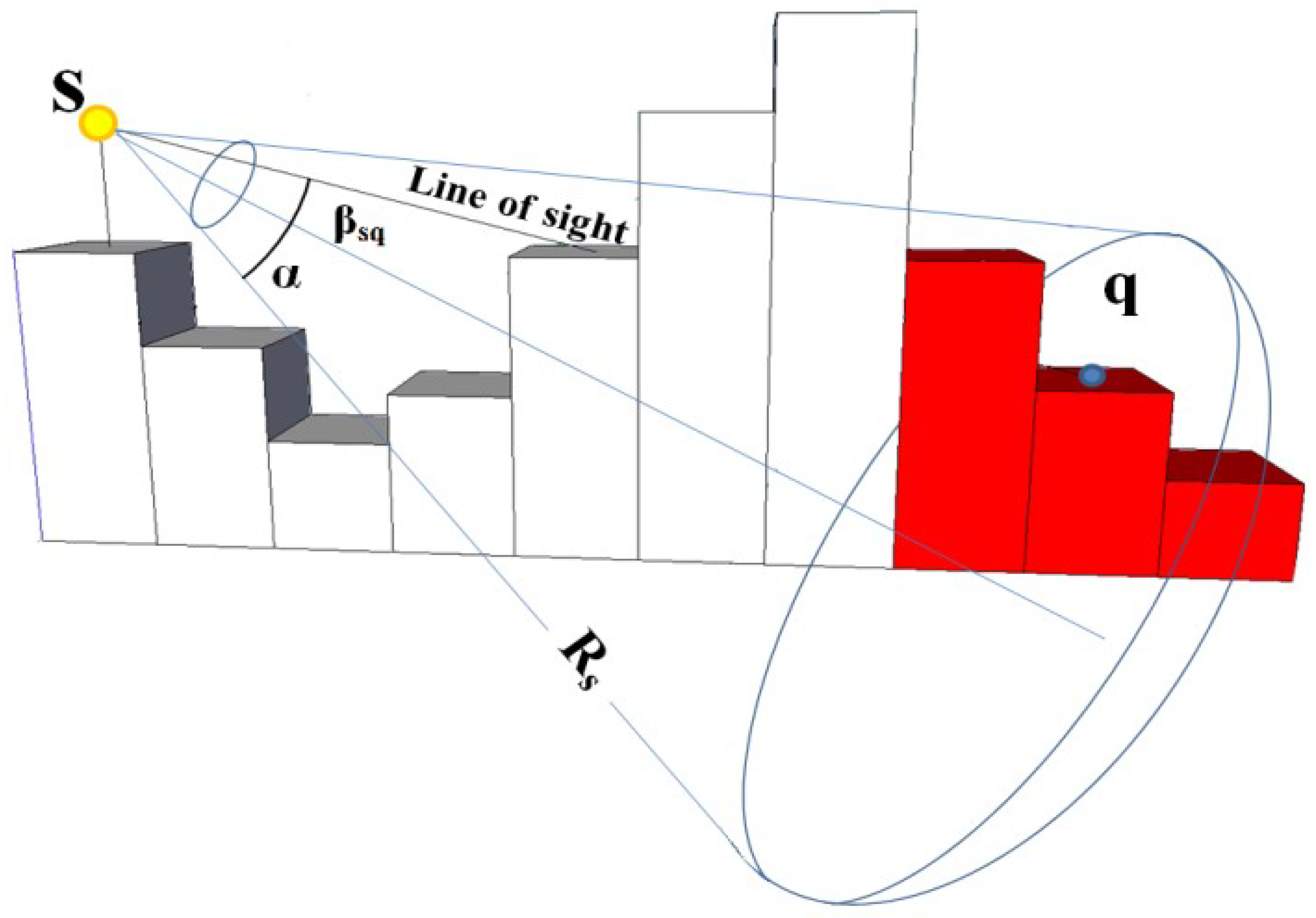
In three-dimensional raster model (Figure 3), we should review the visibility between sensor and pixels regarding the presence of obstacles and topography, besides angle restriction, and performance distance of sensor to compute the sensor coverage.

Hence, the coverage condition of each pixel q is reviewed. In the following condition, pixel q is covered by the sensor S.

$$\{\begin{array}{c}distance\left(S,q\right)\le Rs\\ {\beta }_{sq}\le \alpha \\ visibility\left(S,q\right)=1\end{array}$$

(3)

To investigate the visibility between sensor and pixels, the line of sight is used [36]. The algorithm of line of sight uses the height of each pixel in DSM model to determine the visibility of one pixel through sensor, which is itself located in another pixel. This visibility depends on some parameters, among which we can refer to position and height of sensor, position and height of pixel, orientation of sensor, detection distance of sensor, line of sight and position of obstacles. All of these parameters are simply extractable from three-dimensional model of GIS to review the visibility.

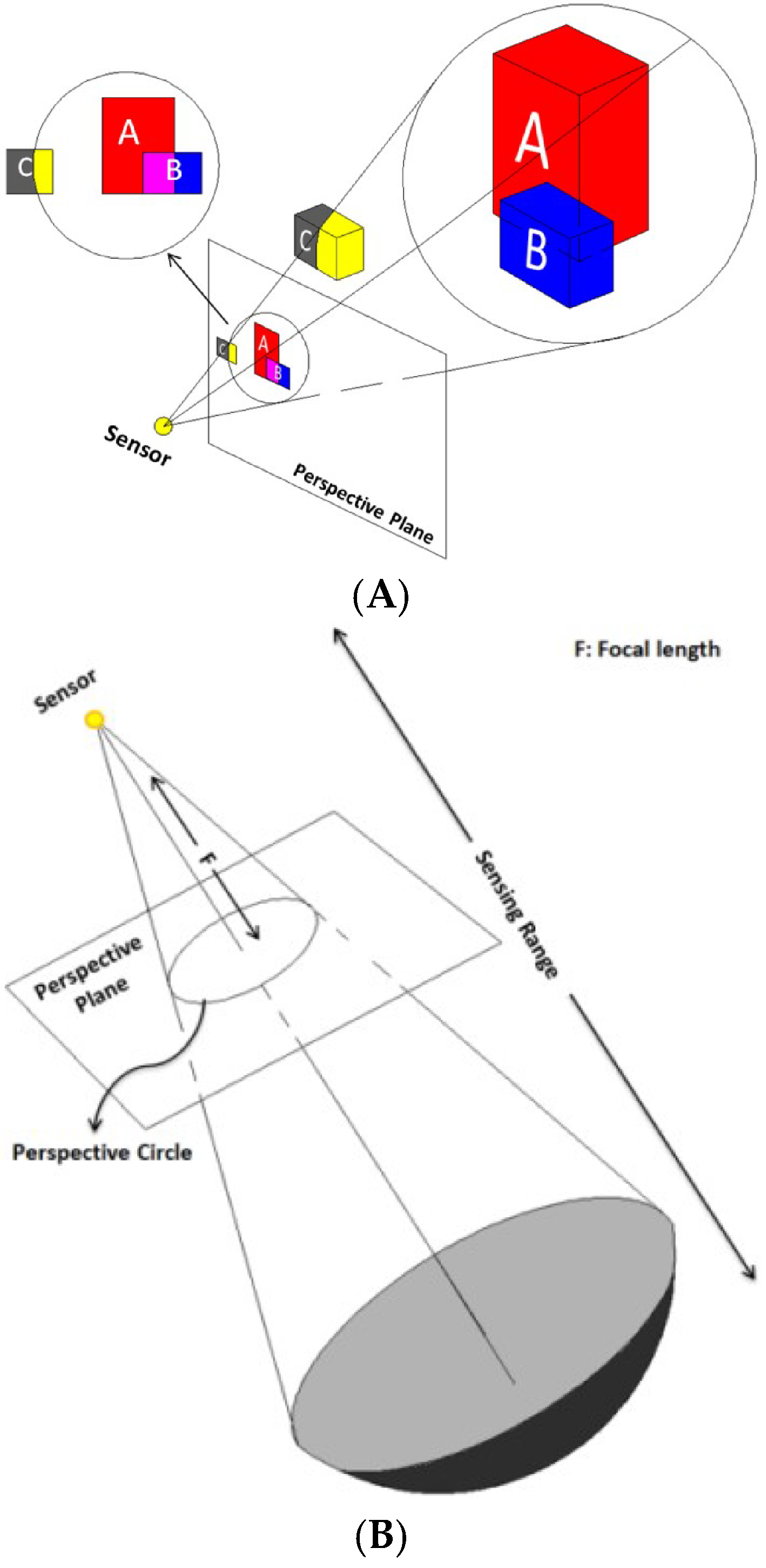
In two-dimensional vector model, the surrounding of sensors is defined as a flat plate restricted to a rectangle. Each polygon is made up a set of line segments. In the proposed method to compute the coverage value, we should first identify the line segments and arcs visible by sensor, and then, it is necessary to collect the area of sectors and triangles resulted from identified arcs and line segments to compute the coverage rate. Finally, in three-dimensional model, the environment is modeled based on City GML Standard, which contains a collection of objects, each made up of a set of polygons. Three-dimensional polygons are ordered according to the farthest distance from the sensor up to the nearest distance from it. According to Figure 4A, a polygon which is towards sensor and is located in the performance range of sensor, is figured on the perspective surface (which is a flat plate perpendicular to the sight direction of sensor, as such that the distance of this plate to sensor is a definite and predetermined rate) [37]. If the figured polygon is located in the perspective circle, it is super-positioned on the polygons existing in the new list. The polygons, which are hidden from sensor’s sight through other polygons, should be removed. Accordingly, the polygons, which passed the previous steps, and were not removed, are figured on perspective plate according to perspective geometry. The polygons figured on the two-dimensional plate of perspective are classified as following:

(1) The polygons that are totally located in the perspective circle are considered as visible polygons (polygon A and B). (2) Polygons that are totally outside of the perspective circle are not in the range of sensor’s performance angle. (3) Polygons that interrupt the perspective circle have some visible parts (polygon C). The visible parts of these polygons are extracted through their interruptions with perspective circle (Figure 4B) [38]. Then, all figured polygons are transferred to three-dimensional space and their areas are computed.

Probability Coverage Model

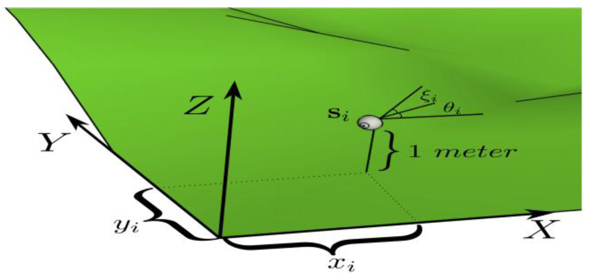
The measurement model of sensor coverage basically depends on the distance, direction and visibility. The coverage C(S_i,q) from sensor S_i at point q in environment is defined by a function from distance d(S_i,q) = $\Vert p_i-q\Vert$, Pan angle p(S_i,q) = ${\angle }_p\left(q-p_i\right)-{\theta }_i$, tilt angle t(S_i,q) = ${\angle }_t\left(q-p_i\right)-{\xi }_i$, and visibility v(S_i,q) of sensor (Figure 5):

$$C\left(s_i,q\right)=f\left[{\mu }_d(\Vert p_i-q\Vert ),{\mu }_p\left({\angle }_p\left(q-p_i\right)-{\theta }_i\right),{\mu }_t\left({\angle }_t\left(q-p_i\right)-{\xi }_i\right),v\left(p_i,q\right)\right]$$

(4)

where $p\left(q-p_i\right)=\arctan \left(y_q-y_{p_i}/x_q-x_{p_i}\right)$ is the angle between $S_i$ sensor and the point q along x axis, and tilt angle $t\left(q-p_i\right)=\arctan \left(z_q-z_{p_i}/\Vert p_i-q\Vert \right)$ is the angle between $S_i$ sensor and point q along the z axis. In other words, the computation of measurement range, measurement angle and visibility are needed for point q which is covered by sensor $S_i$. Estimation of coverage in binary model is more unrealistic than what happens in reality. In probability model, two main distances are considered for the sensor. The first distance $R_s$ (radius of sensor performance) is like binary model. If the distance of objective to sensor is less than $R_s$, the objective is traced with probability of 1. The second distance is Ru. This distance specifies the uncertainty range. If the distance to sensor is between $R_s$ and $R_s+R_u$, the probability that the objective is traced by sensor depends on the distance between them. If the distance between the objective and sensor is more than $R_s+R_u$, the objective will not be traced by sensor. Regarding the range of direction, whatever the direction between sensors towards objective makes more angle with the direction of sensor, the probability of traceability is reduced. Figure 6 shows the probability measurement model.

Equations (5) shows the distance probability and Equation (6) shows the equation of direction probability, and the performance of this model.

$$Pd\{\begin{array}{c}1, Dts\le Rs\\ \frac{1}{1+\exp \left[-\left(\frac{\mathbf{\lambda }}{a}+\mathsf{ß}\right)\right]}, Rs<Dts\ll \mathrm{Rs}+\mathrm{Ru}\\ 0, \mathrm{Rs}+\mathrm{Ru}<Dts\end{array}$$

(5)

$$Pa={\left(\frac{\cos \left(a-\mathsf{\theta }\right)+1}{2}\right)}^{\mathsf{\omega }}$$

(6)

In the probability coverage model, the distance and directional probability for each pixel in the region towards one sensor have been computed, respectively, by Equations (5) and (6), and they are multiplied together. The obtained probability indicates the coverage probability that one sensor covers one pixel [39].

Ps¡t = Pa¡ × Pd¡

(7)

where Pd¡ and P$a¡$ are distance probability and directional probability of pixel i, respectively.

4. Implementation and Evaluation of Results

In this section, the evolutionary global optimization algorithms consider the network coverage as the objective function for the problem of sensor network deployment. Two- and three-dimensional raster models with different resolutions, and the two- and three-dimensional vector models, as more accurate models, are considered. Moreover, the binary omni-directional model has been considered for sensor model in two-dimensional environment model and binary directional model has been considered for sensor model in three-dimensional environment model. The purpose is to achieve the maximum coverage of sensors, which is obtained by regarding to the coverage percentage of all sensors of the region. In this research, algorithms update their own solutions regarding the coverage percent (objective function), which is the proportion of covered area to the maximum coverage power of sensors in the region. For the problem of wireless sensor network deployment, the amount of optimal coverage, the accuracy (by computing coverage in vector model), and convergence speed are considered as the criteria to assess the algorithms. In addition, the solutions of global optimization algorithms are upgraded based on the coverage probability objective function. The criteria of the probability coverage percentage and convergence speed are related to their assessment. The models considered for the sensor and environment are omni-directional sensor model in two-dimensional environment model, and directional model of sensor in three-dimensional environment model. The sensors in this evaluation are considered as CCD cameras, and the sensing and setting parameters were set as a sample CCD sensor. The probability parameters of sensor are, respectively, considered as β = 1 and α = 10 for the distance probability performance and ω = 3 for the direction probability performance of sensor. These values were set based on real sensor parameters, which meet the intended purpose of considered CCD sensors.

To evaluate algorithms in two-dimensional environment model, a point with dimensions of 180 m × 200 m was considered. In addition, raster and vector models were used as evaluators of environmental model in two-dimensional model (Figure 7). In this region, buildings were considered as obstacles in environment model that their dimensions in various resolutions are different due to their diverse accuracy.

While the three-dimensional model was used for the environment of sensors’ deployment, from a region with dimensions of 200 m × 200 m, a vector three-dimensional dataset with City GML model with two levels of details, and raster model (DSM) were used for different resolutions (spatial features that are structured in five subsequent levels of details in which (LoD0) define a vast regional model and (LoD4) with the most details includes the complications inside the building) (Figure 8). 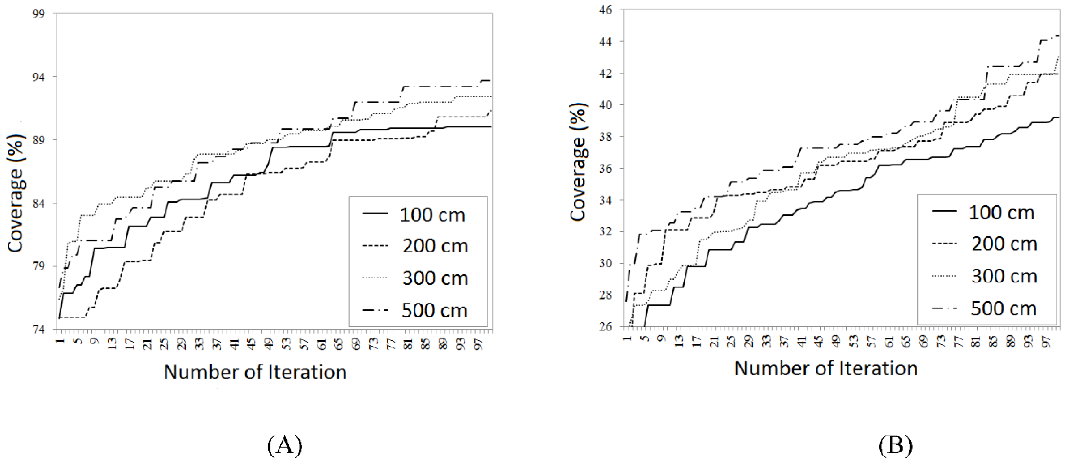All these regions and study samples were extracted from a real city’s (Delft, The Netherlands) topography [40]. This region, besides land topography, contains buildings and trees, which were considered as obstacles. Number of network sensors, as one of the parameters in wireless sensor networks’ deployment, was considered 20. The distance of sensor performance was constant and equaled 15 m. The performance angle of directional sensors was 120 degrees. The interval of sensor height in three-dimensional model for deployment problem as considered as 10 m height (greater height of sensor leads to bigger visibility range due to presence of obstacles). The resolution of two-dimensional and three-dimensional raster models as the environment model of wireless sensor networks’ deployment were assumed as 100, 200, 300 and 500 cm.

The convergence diagram for binary and probability models in raster environment model with different separation models are shown based on global algorithms in Figure 9, Figure 10, Figure 11, Figure 12, Figure 13, Figure 14, Figure 15 and Figure 16. In

Table 1. Values obtained based on genetic algorithm for two- and three-dimensional models.

Dimension of Environment	Resolution (cm)	Coverage (%)	Vector Coverage (%)	Accuracy of Coverage (%)	Time (s)
Two-dimensional	100	90.039	90.024	0.014	87.858
	200	91.334	91.117	0.216	24.808
	300	92.437	91.008	1.429	13.508
	500	93.724	90.975	2.549	7.288
Three-dimensional	100	39.159	38.682	0.477	122.764
	200	41.932	40.526	1.405	34.883
	300	43.083	40.850	2.232	18.152
	500	44.328	36.921	7.407	9.508

,

Table 2. Values obtained based on CMA-ES algorithm for two- and three-dimensional models.

Dimension of Environment	Resolution (cm)	Coverage (%)	Vector Coverage (%)	Accuracy of Coverage (%)	Time (s)
Two-dimensional	100	97.792	97.494	0.297	79.038
	200	98.237	97.851	0.385	17.851
	300	98.527	94.843	3.683	10.566
	500	99.630	95.794	3.836	6.188
Three-dimensional	100	62.813	61.861	0.951	103.638
	200	64.473	63.291	1.182	28.439
	300	68.839	65.796	3.043	14.143
	500	75.451	65.690	9.761	10.628

,

Table 3. Values obtained based on LBFGS algorithm for two- and three-dimensional models.

Dimension of Environment	Resolution (cm)	Coverage (%)	Vector Coverage (%)	Accuracy of Coverage (%)	Time (s)
Two-dimensional	100	96.914	96.584	0.330	92.196
	200	96.709	93.971	2.738	41.304
	300	95.110	85.759	9.352	22.542
	500	88.24	74.484	13.758	12.312
Three-dimensional	100	50.651	48.805	1.845	132.301
	200	45.784	42.710	3.070	40.030
	300	43.413	37.686	5.727	23.800
	500	36.332	25.915	10.416	16.682

and

Table 4. Values obtained based on VFCPSO algorithm for two- and three-dimensional models.

Environment Dimension	Resolution (cm)	Coverage (%)	Vector Coverage (%)	Accuracy of Coverage (%)	Time (s)
Two-dimensional	100	98.407	98.057	0.349	77.290
	200	98.580	98.464	0.084	17.419
	300	99.207	96.404	2.802	9.301
	500	100.585	97.174	3.411	7.365
Three-dimensional	100	52.400	52.184	0.215	101.580
	200	61.370	61.141	0.228	28.769
	300	62.624	57.707	4.916	13.698
	500	67.906	56.819	11.086	11.173

, the final coverage amount, vector amount, accuracy of coverage and time, computation of coverage by global algorithms are shown. All termination conditions and setting parameters for different four applied global optimization algorithms were set based on literature [22,25,26,30] and authors’ experiments.

4.1. Genetic Algorithm

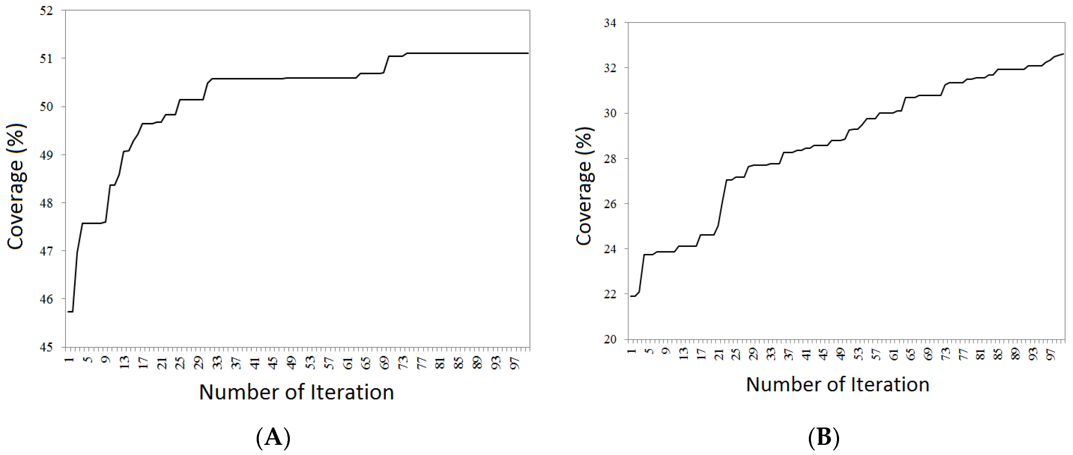
The solutions of genetic algorithms were considered as decimal numbers. Two-dimensional model was implemented by considering the omni-directional sensor model. At first, the omni-directional sensor model was implemented in two-dimensional environment for genetic algorithm. In this case, the solutions were considered as chromosome form. In these solutions, the sensors’ position was assumed as varying parameters. Then, the optimization process of genetic algorithm for three-dimensional model was implemented by directional sensor model. The number of population members in genetic algorithm was considered as 50. The racing selection operator was considered to choose the optimal solution in this algorithm. In the algorithm, the parameter of integration rate, which is used to determine the percentage of present population as the parents for production of new generation, was considered as 70. It means that 70% of population in each repetition are integrated together to produce the next generation.

In fact, this parameter specifies the effect rate of last generation on new generation. In this research, the parameter of mutation rate was considered as 30%. The termination condition was assumed to be 100 repetitions. The final coverage of genetic algorithm of raster model with resolution of 100 cm increases towards the model with resolution of 500 cm. This is because the searching space of model gets smaller by reducing the resolution of model. The convergence diagram of coverage optimization is shown in Figure 9, and the coverage values in Table 1.

The optimal method of research was implemented for the case in which the directional sensor is deployed in three-dimensional environment model; with this difference, their solutions were considered as such that a part of it was related to position parameters and the other part was related to directional parameters of sensor. In this case, height enters chromosomes as the third variable of position.

According to the presented convergence diagrams, the convergence trend of genetic algorithm for two-dimensional model is quicker than three-dimensional model, which is due to presence of more parameters in three-dimensional model. The convergence trend of genetic algorithm in all raster models with different resolutions is the same.

In the following, the optimization of probability coverage has been considered to evaluate the algorithms. Hence, with this purpose, the two and three-dimensional environment models and directional and all-direction model of sensor were implemented for assessment. The convergence trend of coverage optimization trend is shown in Figure 10.

The convergence diagram of this case also greatly specifies the difference of two- and three-dimension models trend. The obtained coverage percentage reduced in comparison to binary case. It is due to computing the coverage probability, which is lower than binary mood.

4.2. CMA-ES Algorithm

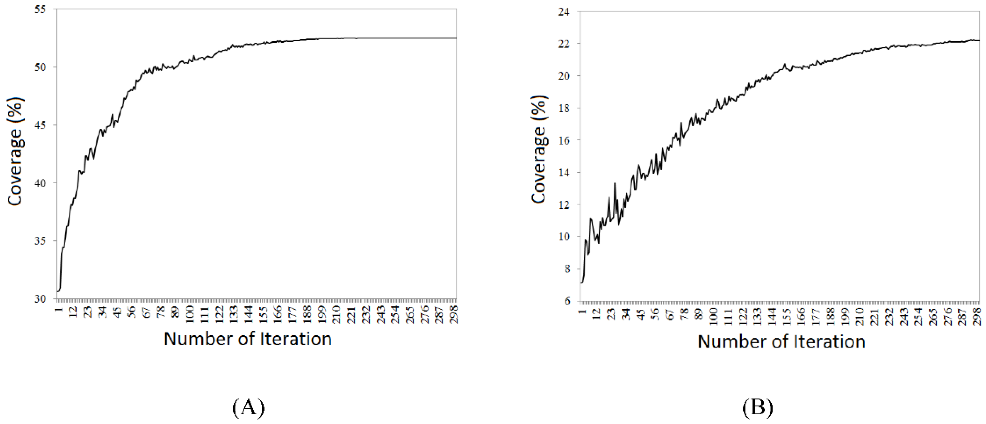
CMA-ES algorithm is an evolutionary algorithm based on population methods. In CMAE-S algorithm, the population parameter λ was considered as 3 + 4 [ln (n)], in which n is the number of variables. To optimize the solutions, CMAE-S algorithm considers the covariance matrix of solutions. Covariance matrix and mean of desirable solutions (the generative solution) specify the new space for exploration. Therefore, the parameter that affects the formation of solutions’ mean is the number of generative solutions considered as λ/2. Among the other parameters related to this algorithm, there is the parameter σ that specifies the direction of the algorithm. This parameter was assumed as 0.167. This parameter was considered as 1 for two-dimensional positions. Ultimately, the termination condition of this algorithm was considered as 300 repetitions, since it has less population than genetic algorithms. The convergence diagram of coverage optimization is shown in Figure 11, and the coverage values in Table 2.

The convergence speed of CMAE-ES algorithm in two-dimensional model is more than in three-dimensional model. The dispersion of convergence diagram in three-dimensional model is more than that of two-dimensional model. From repetition 177 onwards, the improvement trend in two-dimensional model is reduced while in three-dimensional model the convergence diagram continues its trend with a small balance. The results show that coverage amount in all models have been maximized, which indicates the superiority of this algorithm to other previous algorithms.

Regarding to CMAE-ES algorithm, deployment of probability sensors in the region was implemented by considering the obstacles to reach the higher probability coverage. To compare the improvement trend of this algorithm, its convergence diagram is given in Figure 12.

Regarding the convergence diagram, the appropriate performance of this algorithm was specified. Hence, the coverage obtained in two-dimensional model of this algorithm was more than genetic algorithm.

4.3. L-BFGS Algorithm

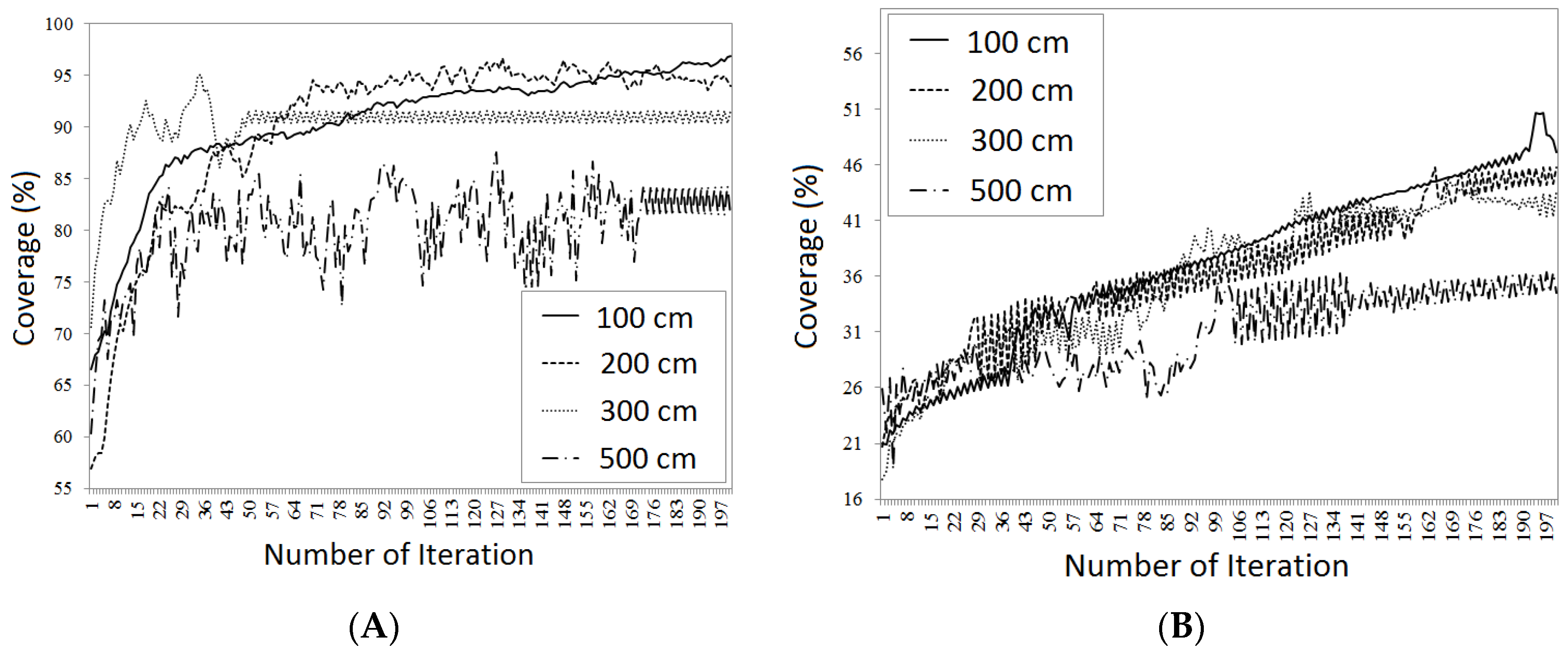
L-BFGS algorithm is a basic gradient algorithm. This algorithm, unlike other algorithms, does not have many parameters, and it just uses its previous m memories to make Hessian covariance matrix. M was considered as 20. To compute gradient numerically, the motion step ε equal to 1 was chosen for two-dimensional positions of sensor. Moreover, the motion step for height variable and directional variable were considered as 0.0056 and 0.0028, respectively. The termination condition of this algorithm was considered as 200, since it uses a solution for optimization of objective function. To compare the raster models with different resolutions, L-BFGS algorithm was implemented for two- and three-dimensional models.

Their convergence model with the termination condition of 200 repetition is shown in Figure 13. The results show that, despite previous methods, the overall coverage is reduced by reducing of the resolution. The reason is that it has more discrete spaces in high resolution models. Table 3 shows the obtained values based on LBFGS algorithm.

L-BFGS algorithm was used for two- and three-dimensional models to evaluate the coverage probability assessment. To better evaluate this method, the convergence diagram for two- and three-dimensional models is shown in Figure 14.

In this scenario, the algorithm efficiency in comparison to three-dimensional model does not have proper certainty, because intensive fluctuations in the improvement trend of coverage reduces quick reaching to optimal coverage value. In this algorithm for three-dimensional model, the convergence process takes place slowly since there are many parameters, and to compute the coverage for each parameter regarding previous algorithms.

4.4. VFCPSO Algorithm

VFCPSO algorithm has been made up of combination of VF and CPSO algorithms. CPSO algorithm is proper for problems in which there are many parameters, as it prevents from trapping in local optima. VF algorithms as a complement algorithm is one of the local optimization algorithms which in the problem of sensor deployment, prevents sensor from getting near to obstacles and other sensors.

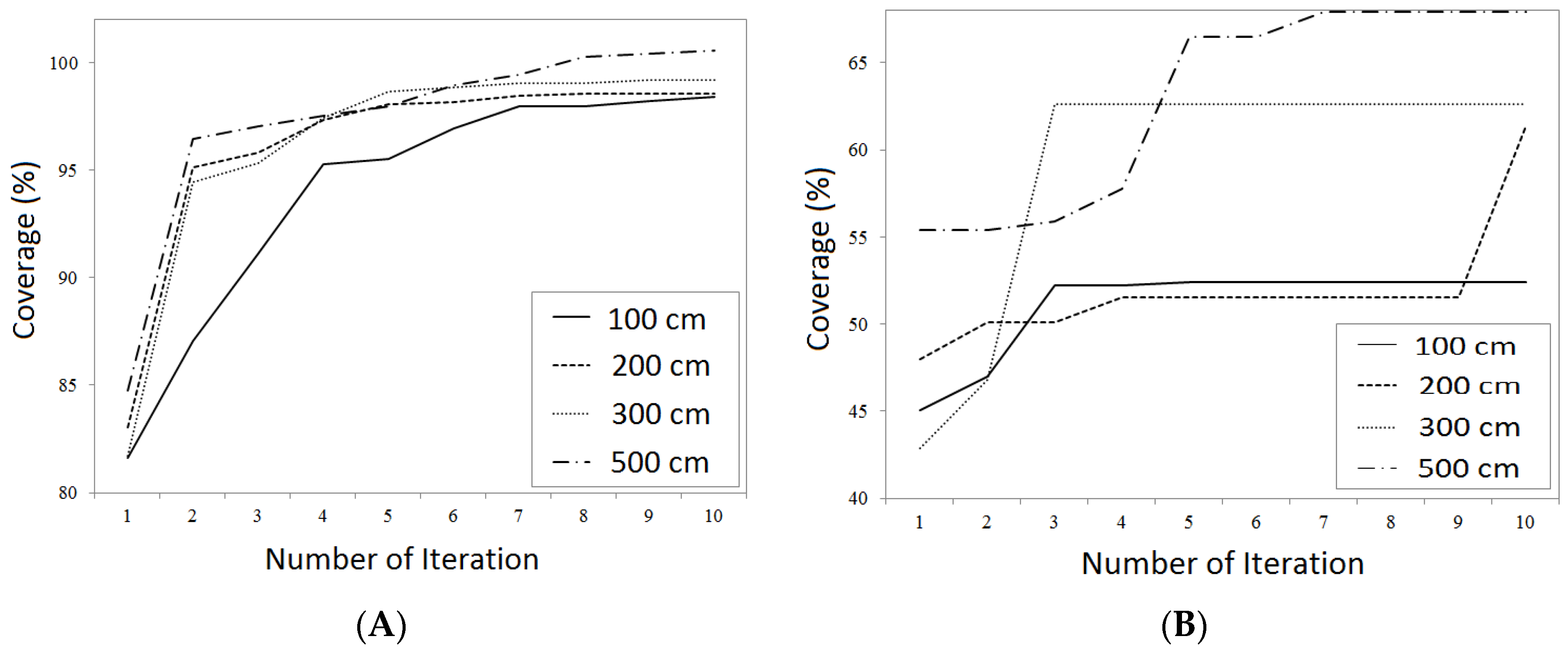
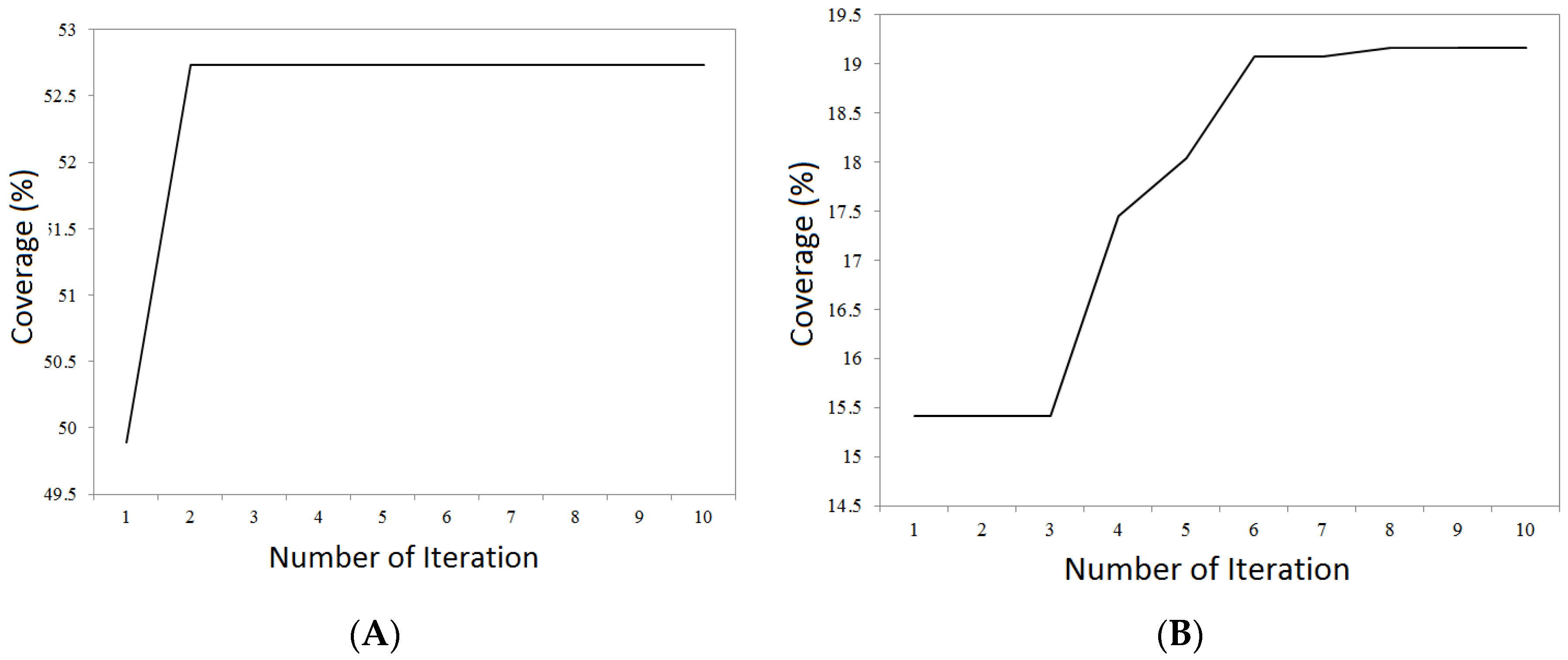
In addition to parameters related to particles’ mass algorithm, the parameters of this algorithm include a parameter as the effect coefficient of VF algorithm in motion speed of particles. This coefficient was considered as 0.2. Since VFCPSO algorithm makes mass as the number of problem’s parameters, the population of each mass was considered as 10. Moreover, its termination condition was considered as 10 iterations. The convergence diagram of coverage optimization is shown in Figure 15, and the obtained values in Table 4.

This algorithm quickly gets near to optimal value. As such, it goes through a proper growth in two iterations, and, after that, the improvement trend moves slowly. The dispersion of convergence diagram is high in three-dimensional model.

In this part, VFCPSO algorithm was used to consider the effect of sensor probability model for two- and three-dimensional raster models. In this respect, convergence diagrams are presented based on two- and three-dimensional models (Figure 16) to better compare the performance of VFCPSO algorithm in the proposed scenario.

Implementation of this scenario based on VFCPSO algorithm and the obtained coverage values show the superiority of this method in terms of reaching a better coverage than other algorithms. In two-dimensional model of this scenario, the algorithm converged quickly, whereas the convergence trend in three-dimensional model has taken place slowly.

In addition to the raster modeling above, the environment of sensor networks was modeled based on the vector coverage for each of the two- and three-dimensional raster models, and their results are shown in Figure 17.

The obtained results of applying different global optimization algorithms indicate that using the proposed models leads to significant accuracy of coverage, which confirms the initial hypothesis of this paper. All four applied algorithms parameters are adapted to enable convergence based on previous simulations. Results show that VFCPSO has the best performance among other proposed optimization methods. Increasing the resolution in both raster and vector models lightly increase the coverage value in all optimization methods. L-BFGS performs slightly worst among other methods, especially when the resolution is low. The other advantage of VFCPSO algorithm is the number of iteration to converge to the optimum coverage compared other methods.

5. Conclusions and Suggestions

In this research, the performance of evolutionary global optimization algorithms were evaluated and compared to make the maximum coverage of wireless sensor networks with the approach of increasing coverage value. Moreover, comparing the results obtained from implementations indicates that, although the examined optimization algorithms in two-dimensional model reached the same results in estimation of probability coverage, their final coverage dropped in three-dimensional model due to high number of parameters in this model.

Moreover, due to twofold local and global approach, VFCPSO algorithm has the best performance among all the implemented algorithms. Since CMA-ES algorithm considers the correlation among solutions’ positions, it has more power in optimizing the coverage value in comparison to its peer, genetic algorithm. L-BFGS algorithm has the most coverage value in raster model with higher resolution, and, in this case, it has a great convergence speed. The running time to compute coverage in three-dimensional model is more than that of two-dimensional model of environment. VFCPSO algorithm possesses shorter running time of coverage computation in comparison to other algorithms.

The other result is that considering the environment with more resolution does not necessarily lead to a better deployment in terms of coverage, since increasing resolution may increase the exploration space of global optimization algorithms and cause that, besides endangering the algorithm to become trapped the local optima, the resolved optima has less coverage. Moreover, increasing the resolution of environment model, the coverage computation processing time for each algorithm decreases. In addition, the final coverage value in three-dimensional model in comparison to two-dimensional model reaches lower value in all algorithms. The reason is the existence of topography, and more parameters of sensor, i.e., height of sensor and direction of component z of sensor in three-dimensional model. By reducing the resolution in raster models, the effect of environmental factors such as obstacles and topography are declined and it makes more errors in coverage computation.

In next steps of this research, the deployment problem will be integrated with the other goals of the network such as communications’ topography, minimum consuming energy, and maximum lifetime. Moreover, the efficiency of global optimization algorithms will be compared by using these aims in more complex environment models. In addition, for future research, we can consider assessment of global optimization algorithms in vector environment model and review the global optimization algorithms in a fixed period together with possessing environment spatial parameters in animated mood and as well as their evaluation by time-spatial approach of spatial information systems.