Development and Experimental Evaluation of a Low-Cost Cooperative UAV Localization Network Prototype


1
Department of Civil Engineering, Indian Institute of Technology Kanpur, Kanpur 208016, India
2
Department of Geospatial Science, RMIT University, Melbourne 3001, Australia
*
Authors to whom correspondence should be addressed.
J. Sens. Actuator Netw. 2018, 7(4), 42; https://doi.org/10.3390/jsan7040042
Submission received: 22 August 2018
/
Revised: 7 September 2018
/
Accepted: 11 September 2018
/
Published: 20 September 2018
(This article belongs to the Special Issue Localization in Wireless Sensor Networks)
Abstract
:Precise localization is one of the key requirements in the deployment of UAVs (Unmanned Aerial Vehicles) for any application including precision mapping, surveillance, assisted navigation, search and rescue. The need for precise positioning is even more relevant with the increasing automation in UAVs and growing interest in commercial UAV applications such as transport and delivery. In the near future, the airspace is expected to be occupied with a large number of unmanned as well as manned aircraft, a majority of which are expected to be operating autonomously. This paper develops a new cooperative localization prototype that utilizes information sharing among UAVs and static anchor nodes for precise positioning of the UAVs. The UAVs are retrofitted with low-cost sensors including a camera, GPS receiver, UWB (Ultra Wide Band) radio and low-cost inertial sensors. The performance of the low-cost prototype is evaluated in real-world conditions in partially and obscured GNSS (Global Navigation Satellite Systems) environments. The performance is analyzed for both centralized and distributed cooperative network designs. It is demonstrated that the developed system is capable of achieving navigation grade (2–4 m) accuracy in partially GNSS denied environments, provided a consistent communication in the cooperative network is available. Furthermore, this paper provides experimental validation that information sharing is beneficial to improve positioning performance even in ideal GNSS environments. The experiments demonstrate that the major challenges for low-cost cooperative networks are consistent connectivity among UAV platforms and sensor synchronization.
1. Introduction
Location awareness is one of the most important requirements in applications such as mapping [1], precision agriculture [2], search and rescue [3], assisted navigation [4], and driverless cars [5]. The European GNSS (Global Navigation Satellite Systems) Agency (GSA) has forecasted that the combined revenue from GNSS devices and augmentation services is expected to grow to about 300 billion Euro by the year 2025, which is about three times the revenue in the year 2017 [6]. This significant growth demonstrates the increasing demand for location awareness in various applications. The GSA has further forecasted that the demand for positioning requirements for UAVs (Unmanned Aerial Vehicles) is expected to grow by about five times from the year 2018 to 2025 with a significant increase in the applications that rely on the use of low-cost UAVs [6]. The FAA (Federal Aviation Administration) estimates that more than of the demands for UAV applications will be met by the lower-end or low-cost UAVs [7]. The FAA defines lower-end UAVs as those UAVs that have an average price of $2500. It is forecasted that in the future low-cost UAVs will characterise the market demand for this technology and technological advancements are needed for meeting the ever-growing demands for positioning of such UAVs.
Existing UAV localization systems rely on GNSS as the primary sensor, ignoring that it is rendered ineffective in urban or obscured environments. Cooperative Localization (CL) provides an alternative framework for localization, using information sharing within a connected network where nodes with GNSS measurements share this information with the other nodes that do not have access to GNSS signals. This information sharing strategy has been demonstrated to be effective in localization of all nodes, irrespective of the availability of GNSS signals to some of the nodes in the network [8]. Additionally, CL is tremendously useful in development and deployment of swarm networks that are robust and significantly more efficient as compared to a single node in applications such as search and rescue, mapping, surveillance, etc. [8].
A cooperative localization framework utilizes a network of inter-connected static and dynamic nodes that share relative information about each other, as well as information about their own states. The static nodes could include available infrastructure such as lamp posts and towers that are equipped with certain communication sensors such as UWB (Ultra Wide Band) and Wi-Fi. A dynamic node is generally a moving platform such as a car, or a UAV that is equipped with positioning and communication sensors. The shared information in such an inter-connected network is used for localization of all dynamic (or even static) nodes, even in GNSS denied environments. Based on the strategy adopted for processing, a CL framework can be divided into two broad categories: centralized [8,9,10,11] and distributed [11,12,13,14,15,16,17,18,19,20,21,22,23,24]. Centralized networks employ a central processor that is responsible for collecting, computing and communicating the states of all nodes in a network. The central processor can be located locally or remotely and needs to maintain constant communication with all the nodes in the network. It is for this reason that the communication and processing requirements in a centralized network are significantly high [8]. The major limitation of centralized networks is that they lack robustness in that they suffer from a single point of failure that includes either the malfunctioning or failure of the processor or the loss of communication link to a single or all nodes to the server. This means that a centralized network would collapse if the processor fails or loses communication with the nodes. Furthermore, centralized networks are generally unscalable and cannot handle the loss or addition of nodes in the network [10,11]. In comparison, distributed networks are scalable, do not require constant communication across the whole network, generally have lower computational requirements which make them more practical for deployment in real-time applications with large number of nodes [8,11,12,25]. Despite the many advantages of distributed networks, their adoption and deployment in real-world applications has been rather limited. Unlike centralized networks, correlations among the states of communicating nodes cannot be estimated precisely in a distributed network [12]. An incorrect estimation or ignoring these correlations has been demonstrated to cause divergence problems in distributed systems [12,26,27]. Therefore, specific algorithms such as the Covariance Intersection Filter (CIF) [17,21], Split Covariance Intersection Filter (SCIF) [20], and Belief Propagation (BP) [16,22,23] have been developed that either estimate or avoid the unknown correlation. Filters such as the CIF and SCIF utilize an optimization method to explicitly estimate the correlations in the states of the nodes using covariance minimization of the fused state. The limitation of this approach is that it requires each node in the network to explicitly estimate the absolute states of the other nodes using relative information collected by its own sensors only [12]. For example, in a CIF or SCIF filter, node A would be required to estimate the position of another node B using relative information collected by sensors onboard the node A. This is possible only if node A is equipped with sensors that are capable of measuring the relative position of node B with respect to node A. This is not possible for cooperative systems that rely on measurements of relative range only and require additional observations such as relative bearing and altitude. Algorithms such as BP and its variants minimize the state correlations by using tree networks. However, the use of tree networks limits the network communication significantly and thus may have an impact on the overall performance. Furthermore, the existing implementations of BP and similar algorithms ignore inertial sensor observations and are generally expensive in terms of communication and processing requirements and thus may not be suitable for real-time applications. Other approaches for distributed estimation in cooperative networks include distributed EKF (Extended Kalman Filter) [13] and MAP (Maximum A Posteriori) [28].
A second classification of CL systems can be done based on their reliance on static anchor (infrastructure) nodes. The CL systems that rely mostly on communication among dynamic nodes (such as cars and UAVs) are referred to as Peer to Peer (P2P) cooperative systems while the systems that rely mostly on static anchors are called Peer to Infrastructure (P2I) systems [29]. A P2I system that is reliant on the presence of already established infrastructure nodes is very useful in urban environments but is rendered ineffective in the absence of infrastructure such as in rural environments and forests. On the other hand, a P2P system is very effective in urban environments as well as infrastructure less environments such as forests. Another limitation of P2I systems is that they require significant investment in terms of development, deployment and maintenance of infrastructure (anchor) nodes. However, P2I based cooperative systems have been demonstrated to outperform P2P networks in terms of the achievable accuracy in cooperative networks. One of the reasons of improved performance in P2I systems is reduced network congestion and availability of a large number of observations from static anchor nodes [29,30,31,32]. It has been demonstrated that the presence of infrastructure anchors in a CL system results in improvement of the overall accuracy and thus the presence of infrastructure anchors in a primarily P2P system is recommended [31].
Some of the different types of relative measurements used in various CL systems include relative range [22,33,34], relative bearing [35], relative position [36], and images with overlapping regions [19,37]. The use of camera images in cooperative localization is based on the detection of common features in the overlapping region to develop relative position constraints among the UAVs in a swarm. These relative constraints are incorporated in a cooperative system to localize UAVs in GNSS denied environments [19]. Significant efforts have been directed towards developing cooperative SLAM (Simultaneous Localization and Mapping) that use either a camera or a LiDAR (Light Detection and Ranging) or a combination of both to cooperatively estimate the localization solution, while simultaneously building a map of the environment [18,36,38,39,40,41,42,43]. The SLAM based methods may provide superior localization performance, but they do so at the cost of increased computational requirements. Furthermore, these methods require the presence of fixed features in the environment and thus their performance might degrade in environments that are devoid of unique features. A majority of the previously mentioned works assume a fully connected network, although it is apparent that network connectivity has an impact on the performance of the overall network. To address this issue, various algorithms have been proposed, either for centralized or distributed networks that attempt to estimate the node states under sparse communication [25,42,44,45]. Some of the recent works have provided experimental demonstrations of including camera observations for cooperative localization in a multi-UAV network [46,47,48]. The authors assume presence of identifiable features in the environment (either indoors or outdoors) that can be tracked in a series of images and provide an experimental validation of their system. This paper develops a low-cost cooperative localization system for UAV swarms that employ ranging systems and evaluates its performance in real-world environments. The performance of the system is evaluated in both P2I and P2P frameworks as well as in centralized and distributed architectures. Using the developed system and extensive experimentation, this paper highlights the challenges in realizing a full scale CL system and provides some recommendations for further improvement.
This paper is organized into four sections. Section 2 discusses the details of the developed cooperative UAV prototype and presents the mathematical framework including various modes of CL for the developed prototype. Furthermore, this section explains the experimental setup for cooperative localization. Section 3 presents and analyzes the performance of the system for different modes and under various operating conditions. The conclusions of this paper and plans for future work are given in Section 4.
2. Materials and Methods
2.1. Cooperative UAV Swarm Network Prototype
The prototype developed in this research integrates low cost sensors including uBloxTM (Thalwil, Switzerland) GPS, Pixhawk autopilot (3D Robotics, Berkeley, CA, USA) that includes MEMS (Micro Electro-Mechanical Systems) gyroscope and accelerometer, P410 UWB radio, Raspberry Pi (Model 3), GoPro camera (San Mateo, CA, USA) and an internet modem for communication and data transmission. The cooperative network developed in this research comprises four such UAVs and about 10 static anchor nodes. Figure 1 lists all the sensors that are installed on any UAV in the developed network. The UWB radio onboard the UAVs allows measurement of range information between the UAVs as well as with infrastructure nodes that are equipped with an UWB sensor. The Raspberry Pi onboard the UAVs is programmed to perform multiple operations. Firstly, it controls some onboard sensors including the UWB and GoPro, stores relevant data from these sensors onboard the SD (Secure Digital) card and monitors the network interactions across different platforms. Secondly, it is responsible for time synchronization of all sensor signals. Thirdly, it transmits all relevant information (i.e., health status) to a master control station (i.e., server) as well as other users. In addition, this Raspberry Pi is capable of recording the RSSI (Received Signal Strength Indicator) measurements from nearby Wi-Fi AP (Access Points) using its internal Wi-Fi adaptor, which can also be included in the CL framework. However, Wi-Fi measurements are not considered in the system design presented in this paper. A schematic diagram showing connectivity and communications among various components onboard the UAV is demonstrated in Figure 2.
The Raspberry Pi is powered by an onboard power bank, UWB has its own dedicated power source while the camera has an inbuilt battery. The power to the Pixhawk is fed from the main UAV battery. The data from GPS and Pixhawk can be transmitted to a laptop on the ground via a telemetry radio. This allows a user to monitor the UAV remotely and identify any faults during the operation. The UWB is controlled by the Raspberry pi and UWB data is stored on the SD card on Raspberry. An image of a UAV prototype in a cooperative UAV swarm developed in this research is shown in Figure 3 and the details of sensors installed on this UAV are given in Table 1. The complete specifications of the onboard sensors including u-Blox GPS, Pixhawk, P410 UWB and GoPro camera are given in [49,50,51,52], respectively. The details of the telemetry radio used are given in [53]. This research uses a commercially available four-arm Octocopter instead of more popular quadcopter models as the unmanned aerial platform. This platform was selected as it is much more stable when compared to a quadcopter, it offers better redundancy in case of motor failure, can fly successfully in windy environments and has a higher payload carrying capacity. The UWB, Raspberry Pi, and GoPro camera are installed at the bottom of the UAV on a stable wooden platform. It can be observed from Table 1 that all the sensors are lightweight and have a small form factor which is very much desirable for UAV applications. The overall weight of the UAV including all batteries and components is about Kg, and the total cost of one UAV is less than approximately $2500. The developed UAV achieves a flight time of about 15 min on a single battery charge. The batteries for the UWB, GoPro, and Raspberry can last for more than 1 h. The Raspberry Pi is field configurable and can be used for performing quality checks on the sensors before flying the UAV. All the UAVs are identical and are equipped with the same sensors. The next section presents the mathematical framework for integration of observations from multiple sensors and multiple platforms using Extended Kalman Filter (EKF).
2.2. Mathematical Details of Cooperative Localization in the Developed Prototype
This section derives the mathematical model for estimating the position of all UAVs in a swarm cooperatively using measurements from neighbouring UAVs as well as static infrastructure nodes. This mathematical framework is based on the EKF but can be extended to an UKF. The objective of the CL framework is to estimate the states of all UAVs after taking into account the relative and absolute measurements received by all UAVs in the swarm. The kinematic mobility model for UAVs in a cooperative swarm is presented first, followed by the measurements models and fusion of measurements in a multi-platform and multi-sensor network under centralized and distributed architectures.
2.2.1. Kinematic Mobility Model
The kinematic mobility model provides a mathematical description of the motion of UAVs. This model incorporates observations from the inertial sensors onboard the UAVs and provides an estimate of the states of the UAVs at a given instant. The state of a UAV i at an instant k in a network containing N UAVs is given by Equation (1):
In the above equation, the 3D position, velocity and attitude of UAV i at instant k is denoted by , , and , respectively. The biases from the accelerometer, gyroscope and GPS receiver clock are denoted by , and , respectively, and the superscript T denotes the transpose of a vector. The rate of change of position, velocity and attitude is governed by Newtonian mechanics and is given by Equations (2)–(4) [8,12]. The following equations are expressed in the ECEF (Earth Centered Earth Fixed) frame which is denoted with a superscript e:
where is given by:
In the above equations, the observations from the onboard accelerometer and gyroscope are denoted by and , respectively. The attitude vector () is composed of roll (), pitch () and () of the UAV and can be expressed in the form . The notation denotes the rate of change of velocity of the UAV. The gravity vector, skew symmetric matrix of earth rotation vector and rotation matrix from IMU (Inertial Measurement Unit) body (denoted by b) to ECEF coordinate system is denoted by , and , respectively. The biases in the accelerometer, gyroscope and GNSS receiver clock are assumed to be Markov and are given by Equations (6)–(8) [8,12,30]:
In the above equations, denotes a random noise and follows any given distribution (e.g., normal distribution). Thus, Equations (2)–(4) and (6)–(8) can be combined to write
where denotes a nonlinear function. The notation u denotes observations from the IMU (i.e., accelerometer and gyroscope measurements) and w denotes the process noise vector. These equations provide the basis for the complete mobility model of a UAV in the developed UAV network. The next section presents a centralized CL framework which incorporates the mobility model and measurements shared within the network to estimate the positioning solution for all UAVs.
2.2.2. Centralized Cooperative Localization
One of the major limitations of centralized networks is that they have a single point of failure (i.e., central server). Despite this limitation, centralized networks can be useful as they can precisely estimate the correlations among the UAV states and may result in a superior localization accuracy as compared to other architectures such as distributed networks [8,12]. Thus, the central server in a centralized network aims to estimate the joint state vector for the overall network. This joint state vector comprises the states of all UAVs in the network and is expressed by Equation (10):
where denotes the state of the ith UAV and is given by Equation (1). This paper proposes to use the EKF for the joint state estimation of all UAVs in the network. A generalized nonlinear mobility model of the form given by Equation (9) can be expressed for the overall centralized network. This nonlinear model is linearized about a nominal joint state using Taylor’s series expansion and is expressed in a discretized form as given by Equation (11):
In the above equation, is a nonlinear function, k denotes an epoch, is the IMU sampling interval, , F is the Jacobian and is given as and is the noise vector. The noise vector is expressed by the following equation:
where denotes the noise vector for a single UAV and can be expressed as follows:
In the above equation, , , , and denote the random errors in the accelerometer and gyroscope observations, and bias parameters for the gyroscope, accelerometer bias and GPS receiver clock, respectively. The transition matrices and for a single node are given by Equations (14) and (15), respectively [8]:
In the above equations, and denote identity and zero matrix, respectively. The matrix and vector in Equation (11) are composed of individual matrices and . These matrices for a single UAV are given by Equations (16) and (17), respectively [10]:
The joint transition matrices and , as seen in Equation (11), take into account the transition matrices of the individual UAVs in a cooperative network and are given by Equations (18) and (19), respectively [8]:
Thus, using Equations (12)–(19) and the initial joint state vector, the joint state of all UAVs at the next instant is computed using Equation (11). It is to be noted that this estimation is performed at the central server and is based entirely on the mobility model explained in Section 2.2.1 and the inertial observations recorded by the sensors onboard the UAVs. The state estimate given by Equation (11) is referred to as the ‘predicted state’. In the absence of any GNSS or relative range measurements between the UAVs, this equation can be used iteratively to compute the joint state at each instant. However, this solution will diverge due to the accumulation of errors in the inertial sensors. Therefore, this predicted estimate needs to be corrected using GNSS measurements received by some (or all) UAVs in the network and/or relative range measurements observed between the UAVs as well as the static nodes.
Consider a UAV i that can receive GNSS pseudorange measurements () from s (≥4) satellites and also observe the relative range () to another UAV j at an instant k. The relative range measurements between two UAVs may be observed using UWB sensors. These absolute and relative measurements received by the ith UAV in a network can be mathematically expressed by Equations (20) and (21), respectively:
In the above equations, the position of the sth GNSS satellite at instant k in the ECEF frame is denoted by , denotes the receiver clock bias and ‖x‖ denotes the -norm of x. The random errors in the GNSS pseudorange and relative distance measurements at instant k are denoted by and , respectively. The joint measurement vector at instant k that encompasses all measurements received by all UAVs in the network is given by Equation (22):
In the above equation, denotes the measurements received by the ith UAV and includes both absolute and relative measurements as given by Equations (20) and (21), respectively. The authors in [8] demonstrated that Equations (20)–(22) can be combined to arrive at the following joint measurement matrix for the complete network:
The above formulation for the joint measurement matrix assumes a fully connected network. In the cases of reduced connectivity, appropriate rows of the above matrix can be removed. In the above matrix, denotes the measurement matrix corresponding to the GNSS measurements received by the ith satellite and can be computed using Equation (24). In this equation, it is assumed that the ith UAV can receive pseudorange measurements from satellites. The notation incorporates the measurement matrix corresponding to the relative range measurements between UAVs i and j. This measurement matrix can be computed using Equation (25):
At this stage, the measurement matrix and joint transition matrices for the complete UAV network are known. Thus, the standard EKF prediction and update equations can be used to jointly estimate the states of UAVs in the network. It is to be noted that the above formulations are adaptive in nature and can take into account the varying connectivity in the network. The maximum size of the measurement vector and matrix in a fully connected network depending on the availability of different types of measurements is given in Table 2.
Although the centralized framework presented above includes observations from inertial sensors and measurements from GNSS and UWB sensors, the same framework can also be adapted to include other additional measurements such as RSS (Received Signal Strength) from Wi-Fi signals. The next section presents the details of a distributed CL framework.
2.2.3. Distributed Cooperative Localization
In contrast to centralized CL, a distributed architecture shares the processing among all the available UAV nodes. The advantage of performing such a decentralization is that the processing requirements do not increase significantly with the increase in the network size [8]. Additionally, distributed architectures are better equipped to take into account the dynamic nature of network size, i.e., removal or addition of UAVs in a cooperative network [12]. One of the major challenges in the successful deployment of distributed networks is the estimation of unknown correlations among the states of interacting UAVs. The authors in [12] presented and provided a first demonstration of their novel distributed localization algorithm that attempts to minimize the correlations among UAV states by imposing additional constraints on the communication in the network. This paper proposes to implement this algorithm in the developed prototype due to its reduced computational requirements. The following provides a complete mathematical derivation and explanation of the EKF based distributed CL strategy.
Let U denote a set of all nodes in a network, G denote a set of nodes that have access to GNSS and denote a set of nodes without GNSS access. The following relationships can be expressed among the three sets:
where denotes the cardinality of set A and ⌀ denotes a null set. The following network conditions are further imposed to ensure that the localization solution of all nodes converge to a precise solution:
The condition in Equation (29) is imposed to ensure that at least one of the nodes without GNSS is able to localize itself by receiving some relative information from the nodes that have access to GNSS. Hence, the condition in Equation (29) is stricter than the one imposed by Equation (28) because, in the absence of Equation (29), the cooperative localization solution would fail. The purpose of introducing the condition given by Equation (28) is to ensure that a larger number of nodes belonging to the set interact with the nodes in set G so that all nodes in set can achieve precise localization. In a fully connected network, Equation (28) would not have much significance, but it can prevent the cooperative solution from collapsing in a sparsely connected network and thus can have a significant impact on the network performance. An important part of this algorithm is the network interaction constraints that attempt to keep the unknown correlation at a minimum. These interaction constraints are given by Equations (30) and (31):
In the above equations, denotes a set of all nodes in the network that are interacting with the node l, and m is one of the nodes in the network that belongs to set . The first constraint allows communication between two nodes only if one of the nodes belongs to set G. The second constraint restricts any communication between the nodes belonging to set . Equations (26)–(31) form the basis of network interaction constraints in the proposed distributed framework.
The proposed distributed framework is based on the EKF and is extendable to the UKF. The advantage of using the EKF is that once the Kalman gain and process covariance matrix is known, standard EKF propagation and update equations can be directly implemented. The measurement vector for the ith UAV that is operating in the absence of GNSS measurements (i.e., ) includes only the relative range measurements received from the neighbouring UAVs and can be expressed by Equation (32) and the corresponding measurement model is given by Equation (33):
In the above equations, denotes a range measurement between node and node and is given by Equation (21), denotes a nonlinear measurement function relating states of nodes i and j, and denotes the noise vector. The measurement model is linearized about nominal states and and can be expressed as
where denotes the Jacobian for the ith UAV. The covariance matrix for ith UAV is given by
where denotes the expectation of x and denotes the true (unknown) estimate of state of node i. The estimate of state of node i can be further expanded to arrive at the following expression:
In the above equations, denotes the Kalman gain and the observed and predicted measurements at node i at epoch k are denoted by and , respectively. Equation (34) is substituted into Equation (36) to arrive at Equation (37) and is given as follows:
The various terms in the above equation can be merged together and rearranged to arrive at the following expression:
Equation (35) is substituted in Equation (38) to arrive the following equation for ,
where denotes the covariance matrix of relative range measurement and denotes Kalman gain. By setting the partial derivative of Equation (39) w.r.t and further re-arrangement, the following expression for the Kalman gain for the ith UAV can be achieved:
Therefore, for a node i that is interacting and receiving information from node j, the covariance matrix of node i is given by Equation (39) and Kalman gain needed for state updation is given by Equation (40). The expressions given in Equations (39) and (40) hold true, if node i is receiving information from one node. In the case, when node i is receiving information from nodes, the expressions for and are given as follows:
In conjunction with the constraints outlined in Equations (26)–(31), the above expressions are used in standard EKF equations for estimating the updated states of all UAVs. The next section provides a simplification of the presented approach in the presence of infrastructure (anchor) nodes and discusses its implications.
2.2.4. Special Case: Infrastructure Based Cooperative Localization
As discussed in the above section, a major challenge in the distributed CL is the estimation of the unknown correlation. The framework presented above provides an alternative solution by limiting the network connectivity in distributed P2P networks. In the presence of a large number of infrastructure (anchor) nodes, such as in urban environments, distributed localization can be further simplified to allow for faster computation. This simplification is achieved by limiting the communication among dynamic (UAV) nodes and allowing such nodes to communicate with static (infrastructure) nodes only. The advantage of this simplification is that correlation among the UAV states is minimized while keeping the processing completely distributed. In addition to this, it is expected that communication load within the network may be reduced by imposing such restrictions. Furthermore, it has been demonstrated that the presence of a large number of infrastructure nodes results in an improvement in the localization accuracy of the UAVs [29].
The infrastructure based CL restricts communication with any two dynamic nodes and only allows a dynamic node to communicate with a static node. If the state of a static node is known in advance, the state of the UAV (i.e., dynamic node) can be estimated using the framework presented in the previous section. Thus, a distributed P2P CL framework can be simplified into two steps in the presence of infrastructure nodes. The first step is called ‘Anchor self localization’ and refers to the estimation of the states of static anchors. The second step pertains to estimation of UAV states using the information about anchor states and is referred to as ‘distributed infrastructure based localization’. Anchor self localization can be achieved either through a manual surveying procedure where the locations of all infrastructure nodes is estimated using standard surveying techniques or through an automatic procedure where anchor nodes communicate with nearby UAVs that have access to GNSS observations to achieve self-localization [11]. Once anchor self localization is achieved, the states of dynamic UAVs can be estimated using information from anchor nodes using the distributed P2P framework presented in the previous section. It can be demonstrated that this framework reduces to standard EKF for the case of infrastructure based CL [12]. This has the advantage that the reduced framework is computationally less expensive than the complete P2P framework.
2.2.5. Adaptive Outlier and Multipath Rejection Algorithm
A preliminary evaluation of the developed prototype demonstrated that the range measurements derived from the UWB sensors onboard the UAVs are corrupted by multipath effects and other outliers [12,30]. An example of the corrupted range measurements as observed by one of the UAVs in a CL experiment is shown in Figure 4. In this experiment, one UWB acts as a static anchor point and is installed on a stable stationary platform on the ground, while another UWB is installed on a UAV that is hovering nearby the stationary UWB. A plot of observed range measurements over time highlights the presence of outliers (marked in orange colour) in the range measurements, as seen in Figure 4. Since the UAV is not completely stationary, minor perturbations in the observed range measurements (18–19 m) can be seen in Figure 4. Additionally, some sudden changes in the range observations are also seen in this figure. For example, the range between a static UWB and UAV changes from about 18 to 12 m in less than 1 s at around 600 s. This is not physically possible since the UAV is hovering at a point. It is hypothesized that this is due to a combination of multipath in the range observations and presence of outliers due to internal sensor electronics. The same UWB behaviour has been reported by the authors in [12,30]. This paper proposes a novel two-step adaptive outlier and multipath rejection algorithm for cooperative networks that can detect and remove such spurious measurements adaptively.The first level detection procedure that identifies the potential measurements that could be corrupted by multipath and other outliers is explained in Level 1. These measurements are then passed on to the second detection step (Level 2) that utilizes a hypothesis testing procedure to detect and remove such corrupted measurements.
Level 1 Detection
The level 1 detection step identifies the potential affected measurements by comparing the rate of change of range measurements with the computed velocity of the UAV in consideration. Consider two different range measurements ( and ) measured by a dynamic UAV ‘s’ with respect to a static infrastructure node at time instants and . Then, the range-rate () can be computed as
Since the velocity of the infrastructure node is zero, the range-rate should always be less than or equal to the velocity of that UAV, i.e., , where ‖a‖ denotes the norm of a vector. In the case, when the range is measured between two dynamic UAVs ‘s’ and ‘p’, the earlier constraint used by the UAV ‘s’ can be modified as follows:
where denotes the range-rate between ‘s’ and ‘p’ and is given by Equation (43). The velocity of the UAV used in this step is taken directly from estimated state available at that instant. If the above constraints are not satisfied, then these range measurements are marked as potentially affected by multipath and are passed to the level 2 detection step.
Level 2 Detection
The first step in this approach is to compute the innovation vector using only the range measurements. The innovation vector at time instant ‘k’ is given as
where and denote the measured relative range and predicted range measurement, respectively. It is to be noted that this innovation vector is computed by the UAVs during processing and is used anyway in the filtering step. Thus, no additional computations are needed to compute this vector. The second step is to check the absolute value of the element of corresponding to the measurement marked in the previous step using Grubb’s test [54]. To implement Grubb’s test, the following two hypotheses are constructed:
- : No range measurements affected by outliers are present in the dataset,
- : At least one range measurement affected by outliers is present.
The above hypotheses are tested using the Grubb’s test statistic. For this specific case, the Grubb’s test statistic is defined as
where , and s denote the value to be checked, sample mean and standard deviation of the sample data Y, respectively. Here, the sample data Y is given by the absolute value of the innovation vector . A one-sided test is used for detecting the multipath corrupted range measurements and the null hypothesis is rejected at a given significance level if,
where denotes the critical value of the t-distribution with degrees of freedom at a significance level of . In order to detect all the affected measurements, this test is run iteratively on the sample dataset. When all the affected measurements have been detected, the remaining measurements are fused using the algorithms described in the earlier sections. This test is terminated when either all measurements marked (by the first level test) have been checked or when the size of the innovation vector is less than or equal to 4. In the case, when the size of the innovation vector is less than 4, level 2 detection cannot be used. The efficacy of this algorithm in improving the localization accuracy in the cooperative network is presented in Section 3.
2.3. Experimental Setup and Ground Truth Estimation
This section presents the details of experimental setup for the evaluation of the developed system and discusses the methodology for establishment of the ground truth. A precise estimation of the ground truth (i.e., reference trajectory) is important because the estimated trajectory solution will be compared against the reference trajectory to evaluate the performance of the system. This paper proposes to use a photogrammetry based approach for the estimation of reference trajectory. The details of the experimental setup are presented first, followed by the methodology for reference trajectory estimation.
2.3.1. Experimental Setup of Cooperative Localization
The cooperative UAV network developed in this paper comprises four UAVs and 10 static anchor points. Each UAV as well as static anchor is installed with a P410 UWB sensor and thus each node can communicate with all the other nodes in the network. For this experiment, the locations of all static anchors is computed in advance using a Leica GS15 GNSS receiver (Heerbrugg, Switzerland) and is embedded in the information being communicated by a static anchor to all the other nodes in the network. An image of the experimental setup for cooperative UAV localization is shown in Figure 5. In this image, one UAV, some anchor nodes, Leica GS15 installed on one of the static anchors are visible. Additionally, some specially designed targets for photogrammetry can also be seen. These targets are used for the estimation of the reference trajectory and their locations are estimated using Leica GS15 GNSS receiver. More details regarding the developed photogrammetric targets is given in Section 2.3.2. Three of the four UAVs and some static anchors can be seen in Figure 6 and a graphical representation of this network at a given instant is shown in Figure 7. The connectivity in the network at this instant is also seen in this figure. It is to be noted that the visualization including network geometry and connectivity shown in this figure is based on the real data collected during the experiments. The connections between the UAVs (referred to as P2P communication) is shown by a red line, while the communication between a UAV and a static anchor is shown by a blue line. It is observed during the experiments and can also be seen in Figure 7 that a fully connected network cannot be realized. This is due to the range limitations of the UWB sensor used in this research. This is significant because the existing literature provides a theoretical evaluation of cooperative networks on the assumption of a fully connected network. The impact of a partially connected network in a cooperative swarm will be discussed in Section 3.
In this experiment, one of the three UAVs (UAV 103) follows a random trajectory as decided by the UAV pilot, while the remaining three UAVs are hovering in a small region. This is done to avoid any potential collisions among the UAVs and to ensure the safety of the equipment and the personnel involved in the experiment. It is to be noted that the assumptions of a hovering UAV or any other constraints on the UAV dynamics are not imposed on the system during processing. A plan view of the trajectory of all UAVs is shown in Figure 8. It can be observed from this figure that UAVs 101, 107 and 200 are hovering in a small region, while UAV 103 is flying all over the region of the experiment. All the UAVs are flown at a height of about 15–25 m from the ground. Some overlap between the UAV trajectories can be observed in Figure 8. To avoid any collision between the UAVs, they are flown at different heights and sufficient vertical separation between them is maintained throughout the experiment. The dynamics of UAV 103 are demonstrated using a plot of the UAV velocity and angular rate, as shown in Figure 9.
It is observed that UAV 103 reaches velocities up to 5 m/s and angular rates up to 2 deg/s. The dynamics of the UAV along the vertical direction are kept at a minimum so as to avoid any collisions with the neighbouring UAVs. The UAVs may be flown at higher speeds but at the risk of either losing control or colliding with the other nearby UAVs or surrounding objects. The number of communicating UWBs available to UAV 103 during the experiment are shown in Figure 10. Although 10 nodes equipped with UWBs are available during the experiment, only eight UWBs could communicate with UAV 103 at any time instant. It can be observed from Figure 10 that 4–6 UWB nodes are available for communication most of the time. Significant loss in communication during the mission operation is also observed. The effect of loss of the communication link in the developed network on the localization performance of the overall network is analyzed and presented in Section 3. In this experiment, the onboard GPS is collecting measurements at 5 Hz, inertial sensors at 100 Hz and UWB sensors at 3 Hz. The GoPro camera is recording images at about 10 FPS (Frames Per Second). All the data is time synchronized and stored on the onboard Raspberry for post processing.
2.3.2. Ground Truth Estimation Using Photogrammetry
This paper proposes to use a photogrammetry based solution for estimation of the reference trajectory. An alternative approach could be to install a precise (and expensive) GNSS receiver onboard the UAV. However, it is not practically feasible because such receivers are bulky and UAVs have a limited payload carrying capacity. Therefore, a light-weight GoPro camera is installed on the UAV which records the images of some specially designed photogrammetric targets that are kept at known locations. Using multiple overlapping images, it is then possible to create a 3D terrain model of the environment as well as estimate the trajectory of the UAV.
This paper uses a checkerboard pattern with known dimensions for performing the camera calibration [55]. The initial calibration is done to arrive at the initial intrinsic matrix of the camera, which is later refined during the pose estimation step. The pattern is imaged by the GoPro camera in various locations and in multiple orientations as shown in Figure 11. The corners in the checkerboard pattern are detected using a Harris corner detector [56]. The detected corners are used in conjunction with a homography estimation method to compute the intrinsic camera matrix. A total of 42 distinct images as shown in Figure 11 are used to estimate the matrix and lens distortion parameters. The detected and re-projected corner points on the checkerboard pattern and the mean re-projection error in each of the 42 images are shown in Figure 12. The maximum mean re-projection error is about pixels and overall mean error is pixels. An overall mean re-projection error of less than one pixel indicates that camera calibration parameters are estimated precisely. This intrinsic camera matrix is used during trajectory estimation and refined intrinsic matrix and reference trajectory is obtained at the end of trajectory estimation step.
This paper uses specially designed photogrammetric targets as shown in Figure 13, for UAV reference trajectory estimation. This research used a total of 18 such unique targets, four of which are shown in this figure. The number at the bottom left corner indicates the ID of the target. The targets are designed to be black in colour so as to ensure better visibility in camera images under bright outdoor conditions. It is to be noted that all the targets are unique and thus different from each other. This uniqueness of targets allows accurate feature matching during the trajectory estimation process. The dimensions and spacing of the targets are estimated keeping in mind the flying conditions and camera parameters. The GoPro camera is operated in 16:9 medium mode with an image resolution of pixels and focal length set to 21 mm. Multiple testing and evaluation of the setup revealed that best results are obtained with a target size of 550 mm × 600 mm, with inner diameter of 100 mm and outer diameter of 500 mm, when the UAV flying height is about 15–25 m. The spacing between the targets is chosen to be about 3–4 m and it is found that a minimum of 4–5 targets are always visible in an image with this configuration. The UAV is programmed to fly at speeds up to 5 m/s and camera rate is set to 10 FPS. Using this setup, more than overlap between two consecutive images is observed in the field. An image of the photogrammetric targets recorded by the GoPro camera onboard a flying UAV is shown in Figure 14. The presence of a large number of such photogrammetric targets in an image is expected to yield better results.
In the image shown in Figure 14, a total of 10 such targets can be easily identified. Such features are detected automatically using SURF (Speeded-Up Robust Features) [57] in multiple images. The outliers in the detected features are removed using the RANSAC (Random Sample Consensus) algorithm [58]. Using the image point correspondences in multiple images and locations of known targets, the 3D scene of the area in the overlapping images is reconstructed [59,60]. The extrinsic camera parameters, i.e., trajectory of the UAV is estimated using bundle adjustment during this step. Since the coordinates of targets are known in a global coordinate system, the reconstructed 3D scene is georeferenced and the UAV trajectory is known in the same global coordinate system. The reference trajectory of the UAV estimated using the described photogrammetric method is shown in Figure 15. In addition, the locations of control points and check points for georeferencing and accuracy evaluation of the estimated trajectory as well as the number of overlapping images used in the estimation are also shown in the same figure. It can be observed from this figure that more than nine overlapping images are available in the majority of the experimental region. This is very much desirable since a larger overlap among images is crucial for achieving better accuracy. A total of seven photogrammetric targets are used as check points, while 11 are used for georeferencing the 3D map and the estimated trajectory. The overall accuracy of the estimated 3D map and the reference trajectory is shown in Table 3. This table demonstrates that the proposed methodology can achieve an accuracy of cm. To further evaluate the accuracy of the estimated trajectory, an n cross validation process [61] is adopted. To perform this cross validation, the set of established photogrammetric targets are divided into two sets, i.e., training set and test set. In the cross validation process adopted here, different combinations of training and test set are considered. Since the accuracy of the estimated trajectory is dependent on the spatial locations of the established training set, not all possible test sets will provide meaningful results. Hence, only those test sets are considered where all the seven check points are not concentrated in one region. The 3D RMSE (Root Mean Square Error) obtained by some of the combinations is demonstrated in Figure 16.
It is observed from the above figure that RMSE for different combinations of control and check points varies from about to cm. Multiple repetitions of the above setup revealed that 3D RMSE achieved using the proposed setup varies from 2 to 4 cm. Thus, it can be inferred that accuracy of the reference trajectory estimated using the methodology explained above is better than 4 cm. The next section evaluates the performance of developed prototype against the reference trajectory estimated using the explained photogrammetric method.
3. Results and Discussion
This section evaluates and analyses the performance of the developed prototype in different scenarios and under different conditions. In this paper, it is assumed that one of the UAVs in the network is operating in the absence of GNSS measurements and is relying only on communication with the other nodes (static or dynamic) for localization. Specifically, it is assumed that UAV 103 (seen in Figure 7) cannot receive GNSS observations. Thus, trajectory of UAV 103 estimated using the presented centralized and distributed frameworks is compared against the reference trajectory to analyze the performance of the developed system. Table 4 summarizes the various cases that are considered for performance analysis in this section.
3.1. Infrastructure Based Localization
An infrastructure based localization framework requires knowledge of the anchor (infrastructure) states. As explained in Section 2.2.4, this can be achieved either through a manual surveying procedure or using an automatic self localization method. In this paper, the locations of anchor nodes are estimated through a manual surveying procedure using a Leica GS15 GNSS. The anchor locations are estimated up to an accuracy of about 5 cm. Although four UAVs are available in the network, the communication among the UAVs is restricted. These UAVs rely only on information sharing with static anchors for state estimation. It is assumed that UAVs are operating in the absence of GNSS measurements. The framework presented in Section 2.2.3 is used to estimate the UAV states. The estimated trajectory is compared against the reference trajectory and a plot of the 3D error in the estimated location of the UAV 103 is shown in Figure 17. The number of infrastructure nodes available for communication to the UAV 103 are also overlaid in this figure. To demonstrate the effect of the developed adaptive multipath and outlier rejection algorithm, the error in the estimated trajectory is plotted before and after inclusion of the multipath rejection algorithm. For better clarity, two zoomed views of this plot are shown in Figure 18 and Figure 19, respectively. From these figures, the first observation that can be made is that the UAV trajectory solution remains bounded even in GNSS denied environments. This provides a first validation that the developed prototype is operating as expected. It can be observed that up to 10 anchor nodes are available for communication at a given instant. The number of UWBs available for communication is not constant and varies from 0 to 10, as seen in Figure 17 and Figure 18. This is due to the dynamic nature of the UAVs and non-availability of direct LOS (Line of Sight) observations. The effect of inclusion of the multipath rejection algorithm is clearly visible in Figure 17, Figure 18 and Figure 19.
The maximum error of about 80 m in the 3D position of the UAV at about 390 s reduces to about 8 m after the inclusion of the multipath rejection algorithm. In the views 1 and 3 marked in Figure 17, the error in the estimated trajectory reduces from 15 m and 25 m to about 5 m, respectively. Furthermore, it is interesting to note that network connectivity has a significant impact on the localization accuracy. The error in the estimated trajectory increases in the absence of any communication with the anchors. For example, from time instant 385 to 390, the error continues to grow until the enough (≥4) number of anchors are available for communication. In the presence of consistent communication in the network, as seen in Figure 19, the localization error stabilizes to about 2–3 m. The same experiment is repeated multiple times and the results are summarized in Figure 20 and Figure 21. It can be observed from these figures that a localization error of less than 5 m is achievable more than of the time using the developed system. It is also seen that the proposed multipath rejection algorithm results in overall improvement of the localization accuracy of the developed prototype. This provides the first experimental demonstration and evaluation of the developed network in GNSS denied environments.
3.2. Centralized Cooperative Localization
In a centralized cooperative network, the states of all UAVs are estimated jointly at a remote central server. Since UAV 103 is assumed to be operating in a GNSS denied environment, its localization performance is analyzed against the estimated reference trajectory to establish the performance of the developed system. A plot of the 3D positioning error in UAV 103, both before and after inclusion of the proposed multipath and outlier rejection algorithm is presented in Figure 22. The number of communicating UWB nodes (both static and dynamic) available to UAV 103 are also shown (scaled by 10) in the same figure. For better clarity, three zoomed views of the same figure (as marked in Figure 22) are shown in Figure 23, Figure 24 and Figure 25. It can be observed from these figures that the connectivity in this network is very poor. This poor connectivity has a significant impact on the localization accuracy, causing the error to grow significantly, when the UAV is operating without any communication with the neighbouring UAVs for an extended period of time. In Figure 23, the error stabilizes to about 4 m in the presence of a consistent communication within the network. This is observed from time instants 10 to 18 s when about 4–6 nodes are available for communication. At other instants, the error continues to vary depending on the availability of communicating nodes, as can be observed in Figure 24 and Figure 25. For example, the error continues to grow between time instants 23 and 26 s due to the unavailability of any UAV or anchor nodes. However, when more than four nodes become available for communication, the error in the estimated solution returns back to about 5 m. The effect of inclusion of the proposed outlier rejection algorithm is clearly visible in Figure 24 and Figure 25.
A large variability in the error in the trajectory solution is observed at multiple time intervals in these figures, in the absence of the multipath and outlier rejection algorithm. This is due to the non-LOS range measurements from some of the nodes (either anchors or UAVs) resulting in multipath and outliers in the observed ranges. A significant improvement in the estimated trajectory is observed after detection and removal of such spurious range observations using the proposed algorithm. For example, the error reduces from about 70 m to less than 10 m at 125 s, 150 m to 50 m at 148 s, and 280 m to less than 20 m at 188 s, as seen in Figure 24. Similar observations about the effect of the developed outlier rejection algorithm can be made in Figure 25. A maximum error of about 400 m in the positioning solution is observed before the inclusion of outlier rejection algorithm. This is due to the combined effect of unavailability of good connectivity in the network and corruption of range measurements by multipath and outliers. This maximum error reduces to about 150 m after including the outlier rejection algorithm in the centralized estimation process.
A comparison of these results with the results presented in Section 3.1 reveals that, although a positioning error of about 2–4 m is achieved in both of the cases, the overall localization performance in a centralized P2P network is significantly poor. This is due to the increased communication load in the centralized network resulting in frequent communication failure. This increase in the communication load is due to the presence of multiple UAVs in a centralized network that are attempting to communicate and share information with each other as well as with the anchor nodes. This is in contrast with a infrastructure based localization framework where the communication between two UAVs is restricted. Nevertheless, it has been demonstrated that a positioning solution accurate to 2–4 m is achievable by centralized P2P networks in partially GNSS denied environments, provided a good communication link can be established among UAVs for an extended period of time. The overall performance of centralized networks in this case is limited by the use of low-cost UWBs. This performance can be significantly improved by the use of better quality communication sensors. The next section presents and discusses the results of CL in distributed networks.
3.3. Distributed Cooperative Localization
In a distributed cooperative network, each UAV performs its own state estimation locally while taking into account the network interactions and the measurements received by each UAV. This estimation is performed using the framework presented in Section 2.2.3. Similar to the previous section, it is assumed that UAV 103 is operating in a GNSS denied environment and relies on communication with other UAVs and static anchors for state estimation. A plot of the localization error for UAV 103 is demonstrated in Figure 26. The results are presented before and after inclusion of the multipath and outlier rejection algorithm. Additionally, the number of UWB nodes (scaled by 10) available to UAV 103 for communication are also shown in the same figure. For better clarity, three zoomed views of this figure are shown in Figure 27, Figure 28 and Figure 29.
Similar observations as in the previous section can be made from these figures. It is observed that localization error is dependent on the connectivity in the network and number of available communicating nodes. When sufficient numbers of communicating nodes are available, the positioning accuracy stabilizes to about 2–4 m (see Figure 27). In the absence of enough communicating nodes, the positioning error degrades but returns to around 4 m when enough nodes become available. The effect of the outlier rejection algorithm is also very clearly visible. The inclusion of the outlier rejection algorithm results in an improvement of the positioning error from about 180 m to 20 m between time instants 175 and 185 s, as can be observed in Figure 28. The combined effect of corrupted range measurements and unavailability of sufficient communicating nodes causes the error to go beyond 500 m at certain instants. However, this error is reduced to about 50 m after removal of the corrupted observations using the developed algorithm, as can be seen in Figure 29.
A comparison of the results of the distributed network with those of the centralized network and infrastructure based localization reveals interesting insights. It can be observed that, although the distributed network achieves an accuracy of 2–4 m, which is similar to that achieved by a centralized network, the distributed positioning solution degrades much faster as compared to centralized localization in the case of a sparsely connected network. This is because the proposed distributed algorithm limits the communication among the UAVs to minimize the correlation among the UAV states. This limitation on the UAVs in a sparsely connected distributed network results in further degradation of the communication quality and thus decreases the quality of the positioning solution. It is then evident that the accuracy achieved in an infrastructure based CL system is much better than a distributed P2P network. However, it is to be noted that the proposed distributed algorithm performs at par with a centralized network and infrastructure based system when the communication in the network is consistent for extended periods of time, typically more than 8–10 s.
3.4. Special Case: Cooperative Localization in Ideal GNSS Environments
The previous sections have presented the performance of the developed system in GNSS denied or partially GNSS denied environments and have demonstrated that the system can achieve accuracy of about 2–4 m, if the communication among nodes is maintained for at least 10 s. This section considers a special case of ideal GNSS environment and presents the localization performance of the system when GNSS is available to all the UAVs throughout the mission. The objective of performing this analysis is to examine the effect of information sharing (such as in a cooperative network) in a full GNSS available environment. This case is presented only for a centralized cooperative network. This is because the proposed distributed algorithm is designed to be applicable only in the cases of partial GNSS availability and it operates as a standard EKF in ideal GNSS environments. In a network with full GNSS availability, the proposed distributed algorithm would prohibit UAVs from interacting with each other and thus each UAV would operate without cooperation.
To analyze the effect of information sharing in a cooperative network in a fully GNSS available environment, the positioning solution for UAV 103 in a cooperative network is compared with the case when this UAV is operating without any cooperation. A CDF plot of the localization error for UAV 103 with and without cooperation is demonstrated in Figure 30. It can be observed that the cooperative solution is marginally better than the trajectory solution of a single UAV operating alone. A cooperative solution achieves an accuracy of up to 2 m about of the time while a single UAV achieves this accuracy about of the time. The reason for this marginal improvement is the inconsistency in the network connectivity in a cooperative network. It is expected that this improvement would be significant if a consistent network connectivity and constant information sharing is achieved in the network.
The same observations can be confirmed from an independent repetition of the above experiment. A CDF plot of the localization error for both the cases (with and without cooperation) is shown in Figure 31. It is seen that improvement achieved in the positioning accuracy in a cooperative network is marginal. The reason is the same as the previous case: that connectivity in the network is sparse and sharing of relative information is infrequent. Significant improvement in the positioning accuracy can be achieved if consistent connectivity and continuous information sharing in the network is established. This is the first experimental demonstration where the benefit of information sharing in a cooperative network in a GNSS available environment is demonstrated. The next section presents the conclusions of this paper and some plans for the future work.
4. Conclusions
This paper has presented the development of a prototype of a new cooperative UAV swarm localization system using low-cost sensors such as GPS, IMU, UWB and camera. Extensive experiments are conducted to establish the performance of this system in real-world environments. Various cooperative localization modes such as centralized network, distributed network and infrastructure based CL, and different environmental scenarios such as partial and full GNSS availability are considered during the experimental evaluation. The experimental results suggest that developed system can achieve an accuracy of about 2–4 m in the absence of GNSS measurements, provided consistent connectivity in the network is maintained for extended periods of time. The overall performance of an infrastructure based CL is better than a centralized or distributed P2P CL. One of the major reasons for better localization performance in infrastructure based CL systems is reduced network congestion. The reasons for achieving 2–4 m accuracy are multiple and includes the effects due to reduced network connectivity, reduced accuracy of UWB range measurements due to NLOS (Non-Line of Sight) conditions or relatively fast movement of the UAV platforms, and about 2–3 m accuracy of the low-cost GPS sensor on-board the UAVs. In addition, the assumptions of Gaussian process and measurement noise may not be satisfied.
Some of the challenges in the developed system include synchronization of the UWB sensors and frequent loss of connectivity in the network. The developed prototype is useful in applications such as search and rescue missions, surveillance, assisted navigation and situational awareness. The performance of the system can be further improved by replacing low-cost sensors such as GPS and IMU with better quality and relatively costly sensors. The future work is aimed at inclusion of observations from signals such as Wi-Fi and other Signals of Opportunity (SOP), development of better quality low-cost communication sensors and increased autonomy in the developed cooperative UAV swarm prototype. This paper has assumed the observations in the system to be Gaussian in nature and utilized EKF based algorithms for faster computation, which may have an impact on the localization accuracy. The future work addresses the issues of non-Gaussian measurements and the use of other particle based estimation algorithms. The implementation of such algorithms on-board UAVs for real-time applications is expected to be a significant challenge in the upcoming research.
Author Contributions
Conceptualization, S.G., A.K. and B.L.; Investigation, S.G.; Methodology, S.G.; Supervision, A.K. and B.L.; Validation, S.G.; Writing—Original draft, S.G.; Writing—Review and Editing, S.G., A.K. and B.L.
Funding
Salil Goel was supported by the Melbourne Research Scholarship (MRS) of the University of Melbourne, Australia and Melbourne India Postgraduate Academy (MIPA), as well as an institute assistantship by the Indian Institute of Technology (IIT) Kanpur, India.
Acknowledgments
The authors would like to express their gratitude to Surabhi Gupta, Tengku Nuddin and Jelena Gabela for assistance in performing the experiments.
Conflicts of Interest
The authors declare no conflict of interest.
Abbreviations
The following abbreviations are used in this manuscript:
| EKF | Extended Kalman Filter |
| GNSS | Global Navigation Satellite System |
| GPS | Global Positioning System |
| IMU | Inertial Measurement Unit |
| NLOS | Non-Line of Sight |
| P2I | Peer to Infrastructure |
| P2P | Peer to Peer |
| RMSE | Root Mean Square Error |
| SD | Secure Digital |
| UAVs | Unmanned Aerial Vehicles |
| UTM | Universal Transverse Mercator |
| UWB | Ultra Wide Band |
References
- Scherer, S.; Rehder, J.; Achar, S.; Cover, H.; Chambers, A.; Nuske, S.; Singh, S. River mapping from a flying robot: State estimation, river detection, and obstacle mapping. Auton. Robots 2012, 1, 189–214. [Google Scholar] [CrossRef]
- Zhang, C.; Kovacs, J.M. The application of small unmanned aerial systems for precision agriculture: A review. Precis. Agric. 2012, 13, 693–712. [Google Scholar] [CrossRef]
- Georgopoulos, P.; McCarthy, B.; Edwards, C. Location Awareness Rescue System: Support for Mountain Rescue Teams. In Proceedings of the Ninth IEEE International Symposium on Network Computing and Applications, Cambridge, MA, USA, 15–17 July 2010; pp. 243–246. [Google Scholar]
- Ishikawa, T.; Fujiwara, H.; Imai, O.; Okabe, A. Wayfinding with a GPS-based mobile navigation system: A comparison with maps and direct experience. J. Environ. Psychol. 2008, 28, 74–82. [Google Scholar] [CrossRef]
- Fischer, J. The Role of GNSS in Driverless Cars, GPS World. Available online: http://gpsworld.com/the-role-of-gnss-in-driverless-cars/ (accessed on 31 September 2018).
- GNSS Market Report, European Global Navigation Satellite Systems Agency, Issue 5. Available online: https://www.gsa.europa.eu/system/files/reports/gnss_mr_2017.pdf (accessed on 20 June 2017).
- FAA Aerospace Forecast—Fiscal Years 2016–2036. 2016. Available online: https://www.faa.gov/data_research/aviation/aerospace_forecasts/media/FY2016-36_FAA_Aerospace_Forecast.pdf (accessed on 20 June 2017).
- Goel, S.; Kealy, A.; Gikas, V.; Retscher, G.; Toth, C.; Brzezinska, D.G.; Lohani, B. Cooperative Localization of Unmanned Aerial Vehicles using GNSS, MEMS Inertial and UWB Sensors. J. Surv. Eng. 2017, 143, 04017007. [Google Scholar] [CrossRef]
- Gabela, J.; Goel, S.; Kealy, A.; Hedley, M.; Moran, B.; Williams, S. Cramér Rao Bound Analysis for Cooperative Positioning in Intelligent Transportation Systems. In Proceedings of the 2018 Conference International Global Navigation Satellite Systems (IGNSS), Sydney, Australia, 7–9 February 2018; Available online: http://www.ignss2018.unsw.edu.au/sites/ignss2018/files/u80/Papers/IGNSS2018_paper_21.pdf (accessed on 8 May 2018).
- Goel, S.; Kealy, A.; Lohani, B. Cooperative UAS Localization using low cost sensors. ISPRS Ann. Photogramm. Remote Sens. Spatial Inf. Sci. 2016, III-1, 183–190. [Google Scholar] [CrossRef]
- Bal, M.; Liu, M.L.M.; Shen, W.S.W.; Ghenniwa, H. Localization in cooperative Wireless Sensor Networks: A review. In Proceedings of the 2009 13th International Conference on Computer Supported Cooperative Work in Design, Santiago, Chile, 22–24 April 2009; pp. 438–443. [Google Scholar]
- Goel, S. A Distributed Cooperative UAV Swarm Localization System: Development and Analysis. In Proceedings of the 30th International Technical Meeting of the Satellite Division of the Institute of Navigation (ION GNSS+ 2017), Portland, OR, USA, 25–29 September 2017; pp. 2501–2518. [Google Scholar]
- Roumeliotis, S.I.; Bekey, G.A. Distributed multirobot localization. IEEE Trans. Robot. Autom. 2002, 18, 781–795. [Google Scholar] [CrossRef]
- Gholami, M.R.; Gezici, S.; Rydström, M.; Ström, E.G. A distributed positioning algorithm for cooperative active and passive sensors. In Proceedings of the 21st Annual IEEE International Symposium on Personal, Indoor and Mobile Radio Communications, Istanbul, Turkey, 26–30 September 2010; pp. 1713–1718. [Google Scholar]
- Mourikis, A.I.; Roumeliotis, S.I. Performance analysis of multirobot cooperative localization. IEEE Trans. Robot. 2006, 22, 666–681. [Google Scholar] [CrossRef]
- Caceres, M.A.; Penna, F.; Wymeersch, H.; Garello, R. Hybrid GNSS-terrestrial cooperative positioning via distributed belief propagation. In Proceedings of the 2010 IEEE Global Telecommunications Conference GLOBECOM 2010, Miami, FL, USA, 6–10 December 2010. [Google Scholar]
- Hlinka, O.; Sluciak, O.; Hlawatsch, F.; Rupp, M. Distributed data fusion using iterative covariance intersection. In Proceedings of the 2014 IEEE International Conference on Acoustics, Speech and Signal Processing (ICASSP), Florence, Italy, 4–9 May 2014; pp. 1861–1865. [Google Scholar]
- Dong, J.; Nelson, E.; Indelman, V.; Michael, N.; Dellaert, F. Distributed real-time cooperative localization and mapping using an uncertainty-aware expectation maximization approach. In Proceedings of the 2015 IEEE International Conference on Robotics and Automation (ICRA), Seattle, WA, USA, 26–30 May 2015; pp. 5807–5814. [Google Scholar]
- Indelman, V.; Gurfil, P.; Rivlin, E.; Rotstein, H. Distributed vision-aided cooperative localization and navigation based on three-view geometry. Robot. Auton. Syst. 2012, 60, 822–840. [Google Scholar] [CrossRef]
- Wanasinghe, T.R.; Mann, G.K.I.; Gosine, R.G. Decentralized Cooperative Localization for Heterogeneous Multi-robot System Using Split Covariance Intersection Filter. In Proceedings of the 2014 Canadian Conference on Computer and Robot Vision, Montreal, QC, Canada, 6–9 May 2014; pp. 167–174. [Google Scholar]
- Carrillo-Arce, L.C.; Nerurkar, E.D.; Gordillo, J.L.; Roumeliotis, S.I. Decentralized multi-robot cooperative localization using covariance intersection. In Proceedings of the 2013 IEEE/RSJ International Conference on Intelligent Robots and Systems, Tokyo, Japan, 3–7 November 2013; pp. 1412–1417. [Google Scholar]
- Savic, V.; Zazo, S. Cooperative localization in mobile networks using nonparametric variants of belief propagation. Ad Hoc Netw. 2013, 11, 138–150. [Google Scholar] [CrossRef] [Green Version]
- Wan, J.; Zhong, L.; Zhang, F. Cooperative Localization of Multi-UAVs via Dynamic Nonparametric Belief Propagation under GPS Signal Loss Condition. Int. J. Distrib. Sens. Netw. 2014, 2014. [Google Scholar] [CrossRef]
- Priyantha, N.B.; Balakrishnan, H.; Demaine, E.; Teller, S. Anchor-Free Distributed Localization in Sensor Networks. In Proceedings of the 1st international conference on Embedded networked sensor systems (SenSys’03), Los Angeles, CA, USA, 5–7 November 2003; pp. 340–341. [Google Scholar]
- Leung, K.Y.K.; Barfoot, T.D.; Liu, H.H.T. Distributed and decentralized cooperative simultaneous localization and mapping for dynamic and sparse robot networks. In Proceedings of the IEEE International Conference on Robotics and Automation, Shanghai, China, 9–13 May 2011; pp. 3841–3847. [Google Scholar]
- Julier, S.J.; Uhlmann, J.K. A non-divergent estimation algorithm in the presence of unknown correlations. In Proceedings of the 1997 American Control Conference (Cat. No.97CH36041), Albuquerque, NM, USA, 6 June 1997; pp. 2369–2373. [Google Scholar]
- Julier, S.; Uhlmann, J.; Durrant-Whyte, H.F. A New Method for the Nonlinear Transforamtion of Means and Covariances in Filters and Estimators. IEEE Trans. Automat. Control 2000, 45, 477–482. [Google Scholar] [CrossRef]
- Nerurkar, E.D.; Roumeliotis, S.I.; Martinelli, A. Distributed maximum a posteriori estimation for multi-robot cooperative localization. In Proceedings of the 2009 IEEE International Conference on Robotics and Automation, Kobe, Japan, 12–17 May 2009. [Google Scholar]
- Goel, S.; Kealy, A.; Lohani, B. Infrastructure vs Peer to Peer Cooperative Positioning: A Comparative Analysis. In Proceedings of the 29th International Technical Meeting of The Satellite Division of the Institute of Navigation (ION GNSS+ 2016), Portland, OR, USA, 12–16 September 2016; pp. 1125–1137. [Google Scholar]
- Goel, S.; Kealy, A.; Retscher, G.; Lohani, B. Cooperative P2I Localization using UWB and Wi-Fi. In Proceedings of the International Global Navigation Satellite Systems (IGNSS) Conference 2016, Sydney, Australia, 6–8 December 2016. [Google Scholar]
- Goel, S.; Gabela, J.; Kealy, A.; Retscher, G. An Indoor Outdoor Cooperative Localization Framework for UAVs. In Proceedings of the International Global Navigation Satellite Systems (IGNSS) Conference 2018, Sydney, Australia, 7–9 February 2018. [Google Scholar]
- Goel, S.; Kealy, A.; Lohani, B.; Retscher, G. Cooperative Localization of Unmanned Aerial Vehicles: Prototype Development and Analysis. In Proceedings of the 10th International Symposium on Mobile Mapping Technology: Mobile Mapping for Sustainable Development, Cairo, Egypt, 6–8 May 2017. [Google Scholar]
- Penna, F.; Caceres, M.A.; Wymeersch, H. Cramér-Rao Bound for Hybrid GNSS-Terrestrial Cooperative Positioning. IEEE Commun. Lett. 2010, 14, 1005–1007. [Google Scholar] [CrossRef]
- Qu, Y.; Zhang, Y. Cooperative localization against GPS signal loss in multiple UAVs flight. J. Syst. Eng. Electron. 2011, 22, 103–112. [Google Scholar] [CrossRef]
- Giguere, P.; Rekleitis, I.; Latulippe, M. I see you, you see me: Cooperative localization through bearing-only mutually observing robots. In Proceedings of the 2012 IEEE/RSJ International Conference on Intelligent Robots and Systems, Vilamoura, Portugal, 7–12 October 2012; pp. 863–869. [Google Scholar]
- Madhavan, R.; Fregene, K.; Parker, L.E. Distributed heterogeneous outdoor multi robot localization. In Proceedings of the 2002 IEEE International Conference on Robotics and Automation (Cat. No.02CH37292), Washington, DC, USA, 11–15 May 2002; pp. 374–381. [Google Scholar]
- Melnyk, I.V.; Hesch, J.A.; Roumeliotis, S.I. Cooperative vision-aided inertial navigation using overlapping views. In Proceedings of the IEEE International Conference on Robotics and Automation, Saint Paul, MN, USA, 14–18 May 2012; pp. 936–943. [Google Scholar]
- Bryson, M.; Sukkarieh, S. Building a Robust Implementation of Bearing-Only Inertial SLAM for a UAV. J. Field Robot. 2007, 24, 113–143. [Google Scholar] [CrossRef]
- Bryson, M.; Sukkarieh, S. Cooperative Localisation and Mapping for Multiple UAVs in Unknown Environments. In Proceedings of the IEEE/AIAA Aerospace Conference, Big Sky, MT, USA, 3–10 March 2007; pp. 1–12. [Google Scholar]
- Ryde, J.; Hu, H. Cooperative Mutual 3D Laser Mapping and Localization. In Proceedings of the 2006 IEEE International Conference on Robotics and Biomimetics, Kunming, China, 17–20 December 2006; pp. 1048–1053. [Google Scholar]
- Wu, M.; Huang, F.; Wang, L.; Sun, J. Cooperative multi-robot monocular-SLAM using salient landmarks. In Proceedings of the 2009 International Asia Conference on Informatics in Control, Automation, and Robotics, Milan, Italy, 2–5 July 2009; pp. 151–155. [Google Scholar]
- Paull, L.; Huang, G.; Seto, M.; Leonard, J.J. Communication-constrained multi-AUV cooperative SLAM. In Proceedings of the IEEE International Conference on Robotics and Automation, Seattle, WA, USA, 26–30 May 2015; pp. 509–516. [Google Scholar]
- Trujillo, J.C.; Munguia, R.; Guerra, E.; Grau, A. Cooperative Monocular-Based SLAM for Multi-UAV Systems in GPS-Denied Environments. Sensors 2018, 18, 1351. [Google Scholar] [CrossRef] [PubMed]
- Ko, J.; Stewart, B.; Fox, D.; Konolige, K.; Limketkai, B. A practical, decision-theoretic approach to multi-robot mapping and exploration. In Proceedings of the International Conference on Intelligent Robots, Las Vegas, NV, USA, 27–31 October 2003. [Google Scholar]
- Trawny, N.; Roumeliotis, S.I.; Giannakis, G.B. Cooperative multi-robot localization under communication constraints. In Proceedings of the IEEE International Confererence on Robotics and Automation, Kobe, Japan, 12–17 May 2009. [Google Scholar]
- Vetrella, A.R.; Fasano, G.; Accardo, D.; Moccia, A. Differential GNSS and Vision-Based Tracking to Improve Navigation Performance in Cooperative Multi-UAV Systems. Sensors 2016, 16, 2164. [Google Scholar] [CrossRef] [PubMed]
- Vetrella, A.R.; Fasano, G.; Renga, A.; Accardo, D. Cooperative UAV Navigation Based on Distributed Multi-Antenna GNSS, Vision, and MEMS Sensors. In Proceedings of the International Conference on Unmanned Aircraft Systems, Denver, CO, USA, 9–12 June 2015. [Google Scholar]
- Kenmogne, I.F.; Drevelle, V.; Marchand, E. Using constraint propagation for cooperative UAV localization from vision and ranging. In Proceedings of the Constraint Programming and Decision Making Workshop, Tokyo, Japan, 10 September 2018; pp. 1–5. [Google Scholar]
- Specifications of uBlox LEA-6H. Available online: https://goo.gl/HY4bC4 (accessed on 24 November 2017).
- Specifications of Pixhawk Autopilot. Available online: https://pixhawk.org/modules/pixhawk (accessed on 26 August 2016).
- Details of P410 UWB Radio. Available online: http://www.timedomain.com/ (accessed on 31 August 2018).
- Specifications and Details of GoPro Hero 3 Silver Edition. Available online: http://cbcdn1.gp-static.com/uploads/product_manual/file/55/HERO3_Silver_UM_ENG_RevC_web.pdf (accessed on 27 August 2016).
- Details of the Telemetry Radio. Available online: http://ardupilot.org/copter/docs/common-sik-telemetry-radio.html#common-sik-telemetry-radio (accessed on 31 August 2018).
- Grubbs, F.E. Procedures for Detecting Outlying Observations in Samples. Technometrics 1969, 11, 1–21. [Google Scholar] [CrossRef] [Green Version]
- Zhang, Z. A flexible new technique for camera calibration. IEEE Trans. Pattern Anal. Mach. Intell. 2000, 22, 1330–1334. [Google Scholar] [CrossRef] [Green Version]
- Harris, C.; Stephens, M. A combined corner and edge detector. In Proceedings of the Alvey vision conference, Manchester, UK, 31 August–2 September 1988; p. 50. [Google Scholar]
- Bay, H.; Ess, A.; Tuytelaars, T.; Van Gool, L. Speeded-up robust features (SURF). Comput. Vis. Image Underst. 2008, 110, 346–359. [Google Scholar] [CrossRef]
- Fischler, M.A.; Bolles, R.C. Random sample consensus: A paradigm for model fitting with applications to image analysis and automated cartography. Commun. ACM 1981, 24, 381–395. [Google Scholar] [CrossRef]
- Moons, T.; Gool, L.V.; Vergauwen, M. 3D Reconstruction from Multiple Images, Part 1: Principles. Found. Trends Comput. Graph. Vis. 2009, 4, 287–404. [Google Scholar] [CrossRef]
- Larsson, V. Metric 3D-Reconstruction from Unordered and Uncalibrated Image Collections. Master’s Thesis, Lund University, Lund, Sweden, 2013. Available online: http://www2.maths.lth.se/vision/publdb/reports/pdf/larsson-master-13.pdf (accessed on 18 April 2017).
- Kohavi, R. A study of cross-validation and bootstrap for accuracy estimation and model selection. In Proceedings of the 14th International Joint Conference Artificial Intelligence, Montreal, QC, Canada, 20–25 August 1995; pp. 338–345. [Google Scholar]
Figure 1.
Sensors onboard the developed UAV platform.

Figure 2.
Schematic plot showing inter-connections among various components on the UAV.

Figure 3.
Image showing one of the developed UAV prototype in a cooperative swarm.

Figure 4.
Range measurements observed between a static UWB anchor and a hovering UAV.

Figure 5.
Image showing experimental setup for cooperative UAV localization.

Figure 6.
Experimental setup for cooperative localization. Three of the four UAVs can be seen in this image.
Figure 6.
Experimental setup for cooperative localization. Three of the four UAVs can be seen in this image.

Figure 7.
A visual representation of the network geometry at an instant in the developed cooperative swarm network.
Figure 7.
A visual representation of the network geometry at an instant in the developed cooperative swarm network.

Figure 8.
Plan view of the trajectory of the four UAVs in the network.

Figure 9.
Dynamics of one of the UAVs in the experiment. The velocity is shown on the left and angular rates along three directions are shown on the right.
Figure 9.
Dynamics of one of the UAVs in the experiment. The velocity is shown on the left and angular rates along three directions are shown on the right.

Figure 10.
Number of communicating UWBs available to UAV 103 during the experiment.

Figure 11.
Representative images of the checkerboard pattern used for camera calibration.

Figure 12.
Figure showing detected and re-projected corner points after camera calibration (left) and mean re-projection error in the pixel coordinates of all images used during camera calibration (right).
Figure 12.
Figure showing detected and re-projected corner points after camera calibration (left) and mean re-projection error in the pixel coordinates of all images used during camera calibration (right).

Figure 13.
Ground targets for trajectory estimation using photogrammetry.

Figure 14.
Image captured by the GoPro camera installed on one of the UAVs.

Figure 15.
Figure showing the estimated reference trajectory as well as number of overlapping images (left) and spatial distribution of control points and check points for one of the iterations (right).
Figure 15.
Figure showing the estimated reference trajectory as well as number of overlapping images (left) and spatial distribution of control points and check points for one of the iterations (right).

Figure 16.
A plot of RMSE obtained for different combinations of check points and control points.

Figure 17.
Plot of localization error overlaid with number of available UWBs for the first experiment.
Figure 17.
Plot of localization error overlaid with number of available UWBs for the first experiment.

Figure 18.
View2: zoomed view of Figure 17.
Figure 18.
View2: zoomed view of Figure 17.

Figure 19.
View4: zoomed view of Figure 17.
Figure 19.
View4: zoomed view of Figure 17.

Figure 20.
CDF (Cumulative Density Function) plot of localization error for the first experiment.

Figure 21.
CDF plot of localization error for the second experiment.

Figure 22.
Localization error for UAV 103 in the developed centralized cooperative swarm. The number of UWB nodes available to UAV 103 are also shown.
Figure 22.
Localization error for UAV 103 in the developed centralized cooperative swarm. The number of UWB nodes available to UAV 103 are also shown.

Figure 23.
View1: zoomed view of Figure 22.
Figure 23.
View1: zoomed view of Figure 22.

Figure 24.
View2: zoomed view of Figure 22.
Figure 24.
View2: zoomed view of Figure 22.

Figure 25.
View3: zoomed view of Figure 22.
Figure 25.
View3: zoomed view of Figure 22.

Figure 26.
Localization error for UAV 103 in the developed distributed cooperative swarm. The number of UWB nodes available to UAV 103 are also shown.
Figure 26.
Localization error for UAV 103 in the developed distributed cooperative swarm. The number of UWB nodes available to UAV 103 are also shown.

Figure 27.
View1: zoomed view of Figure 26.
Figure 27.
View1: zoomed view of Figure 26.

Figure 28.
View2: zoomed view of Figure 26.
Figure 28.
View2: zoomed view of Figure 26.

Figure 29.
View3: zoomed view of Figure 26.
Figure 29.
View3: zoomed view of Figure 26.

Figure 30.
A CDF plot showing a comparison of the localization solution of the UAV in a cooperative network versus when operating alone.
Figure 30.
A CDF plot showing a comparison of the localization solution of the UAV in a cooperative network versus when operating alone.

Figure 31.
A CDF plot showing a comparison of the localization solution of the UAV in a cooperative network versus when operating alone for another repetition of the same experiment.
Figure 31.
A CDF plot showing a comparison of the localization solution of the UAV in a cooperative network versus when operating alone for another repetition of the same experiment.


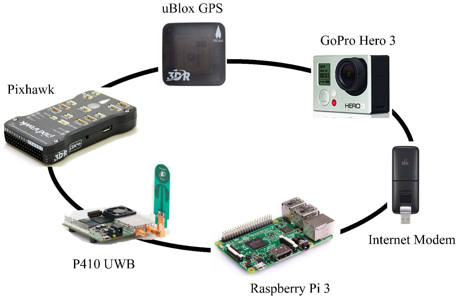
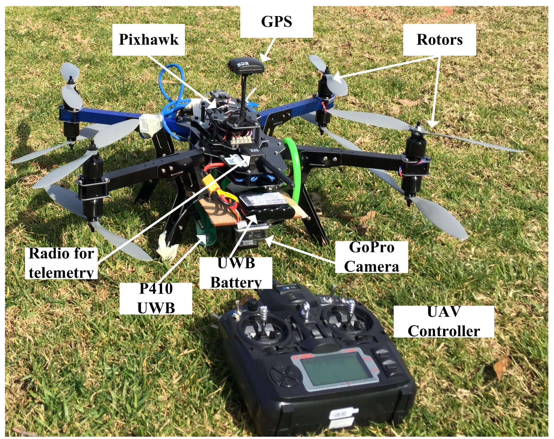
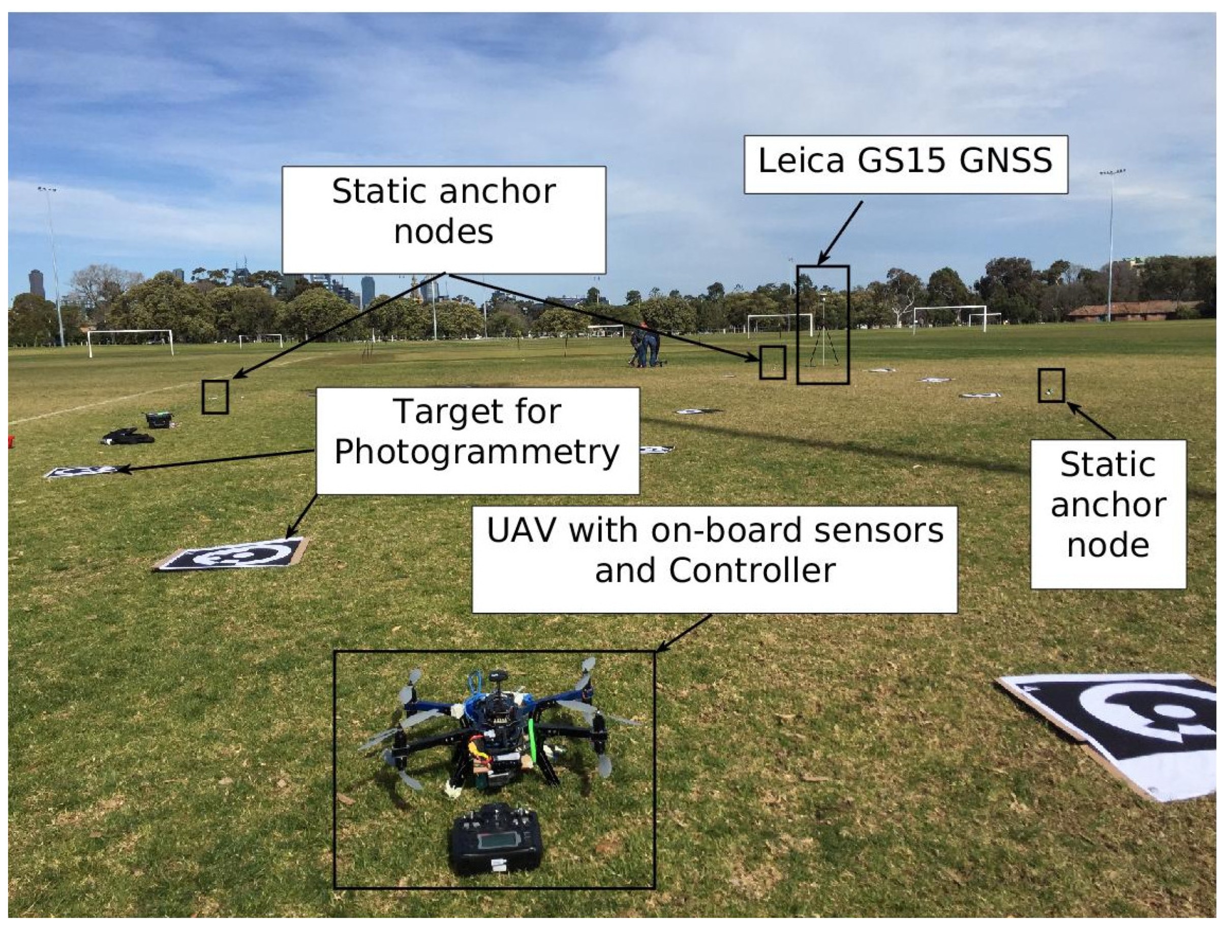
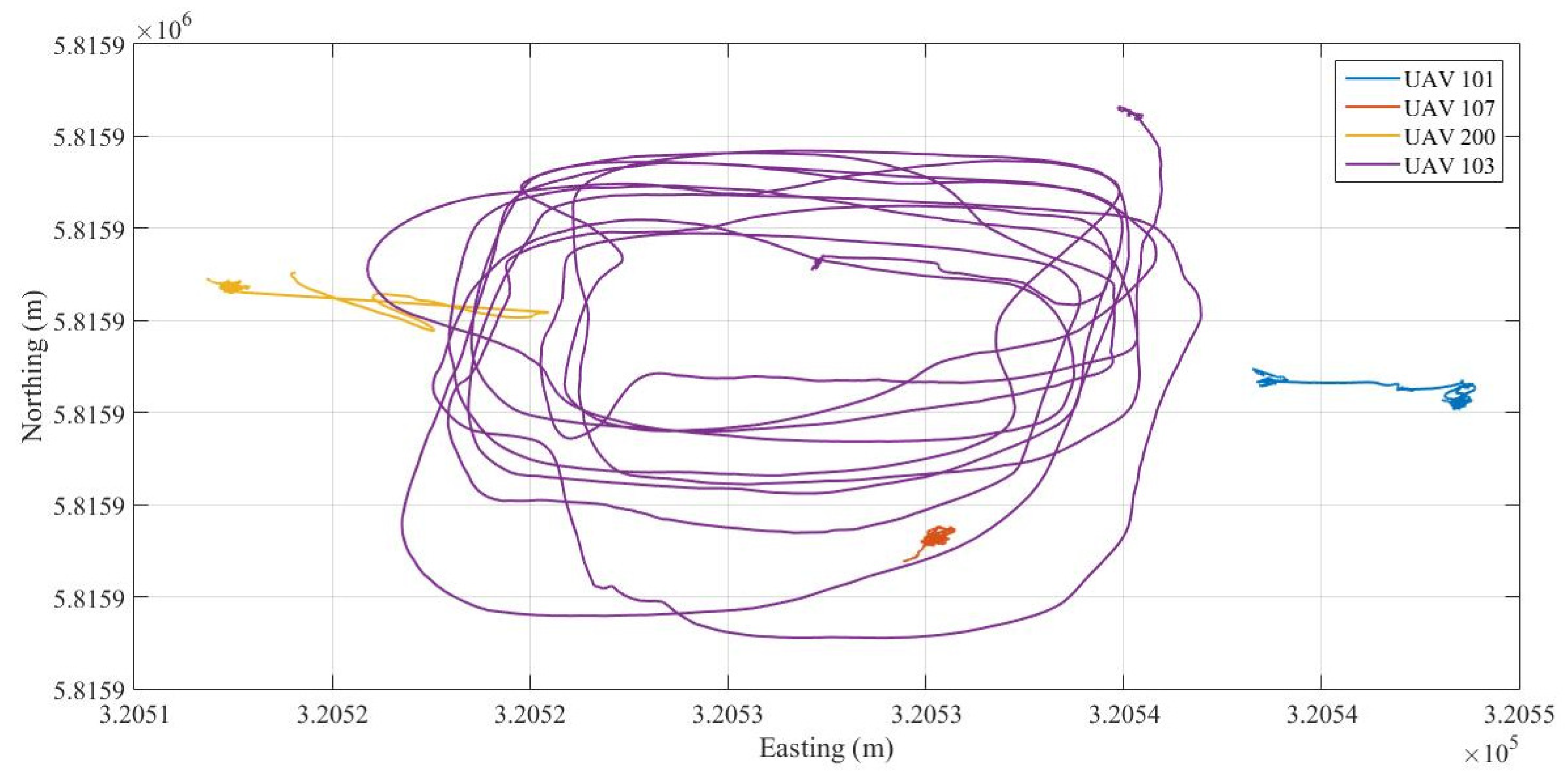
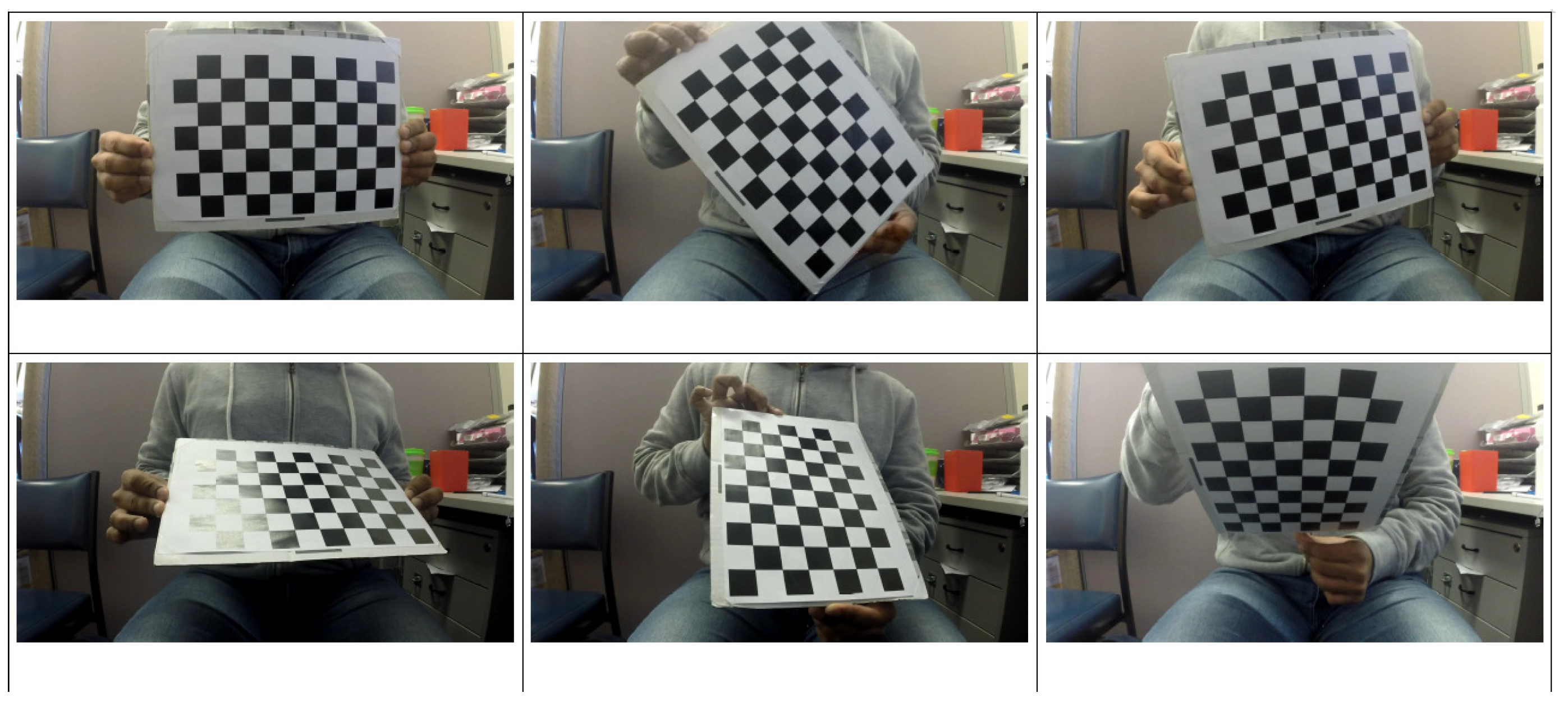
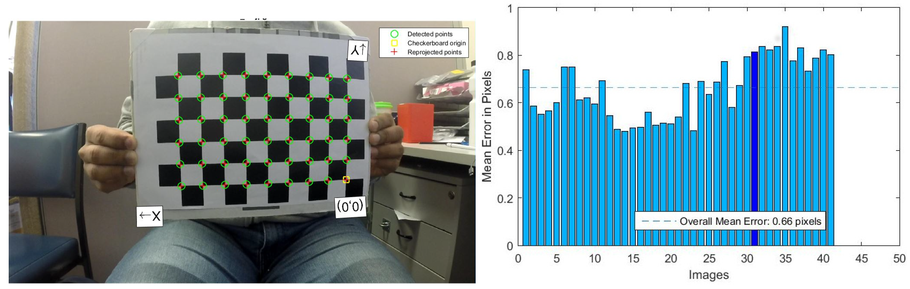
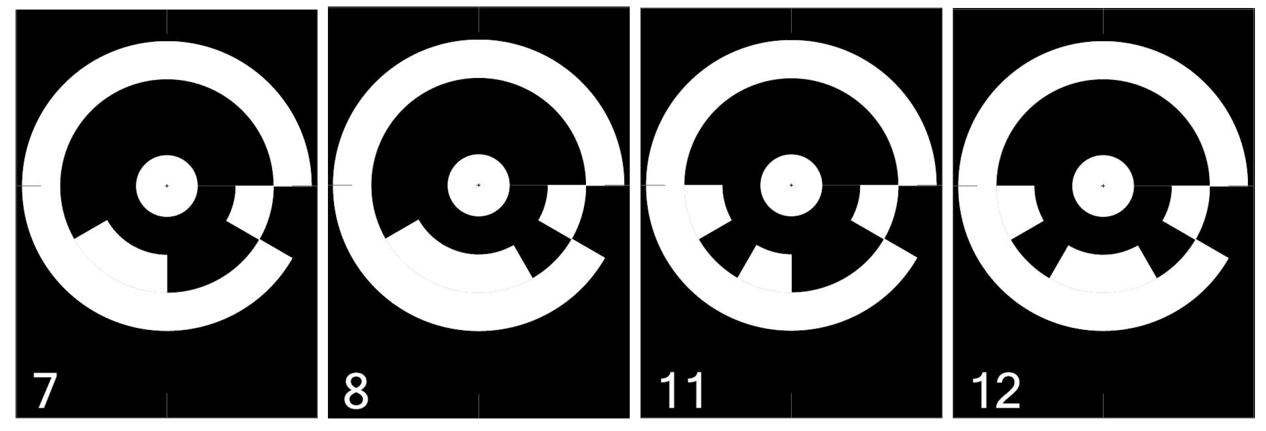
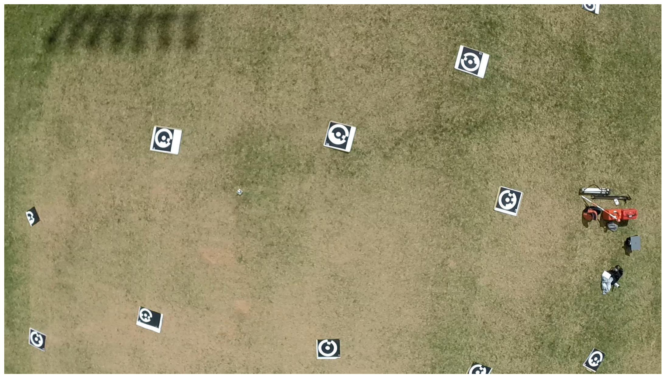
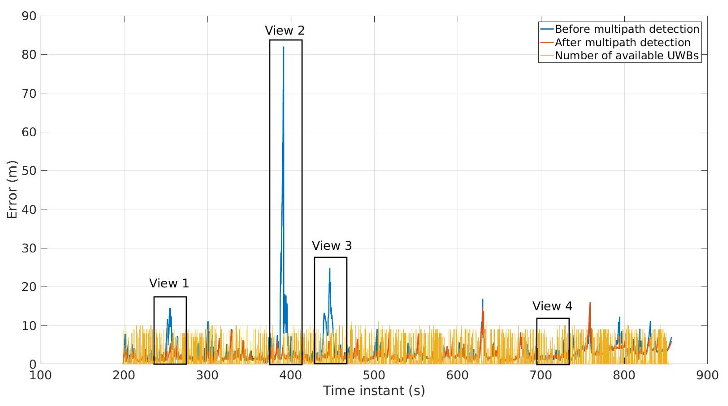
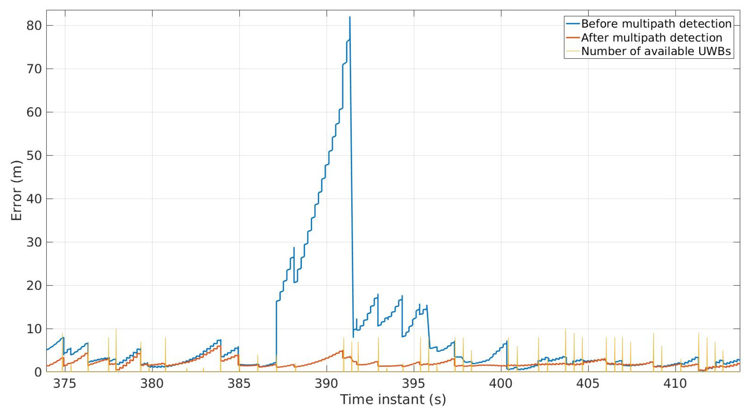
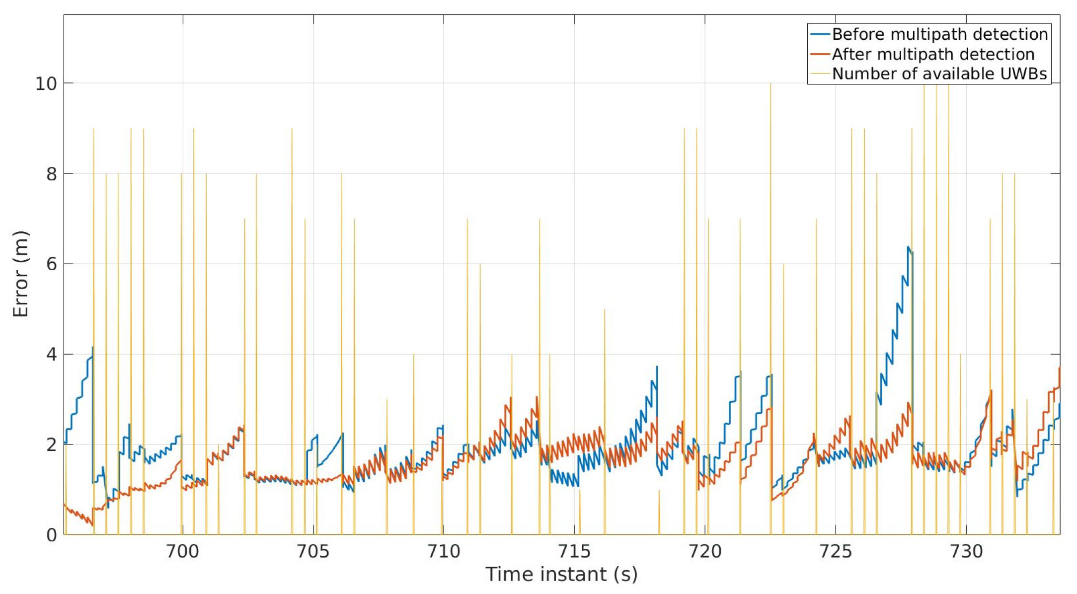
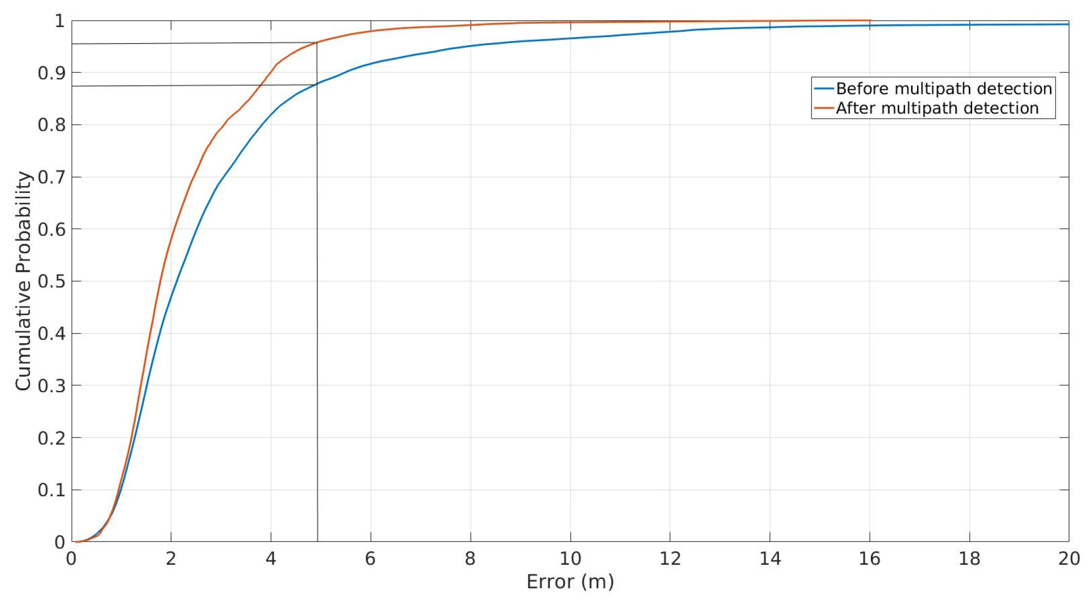
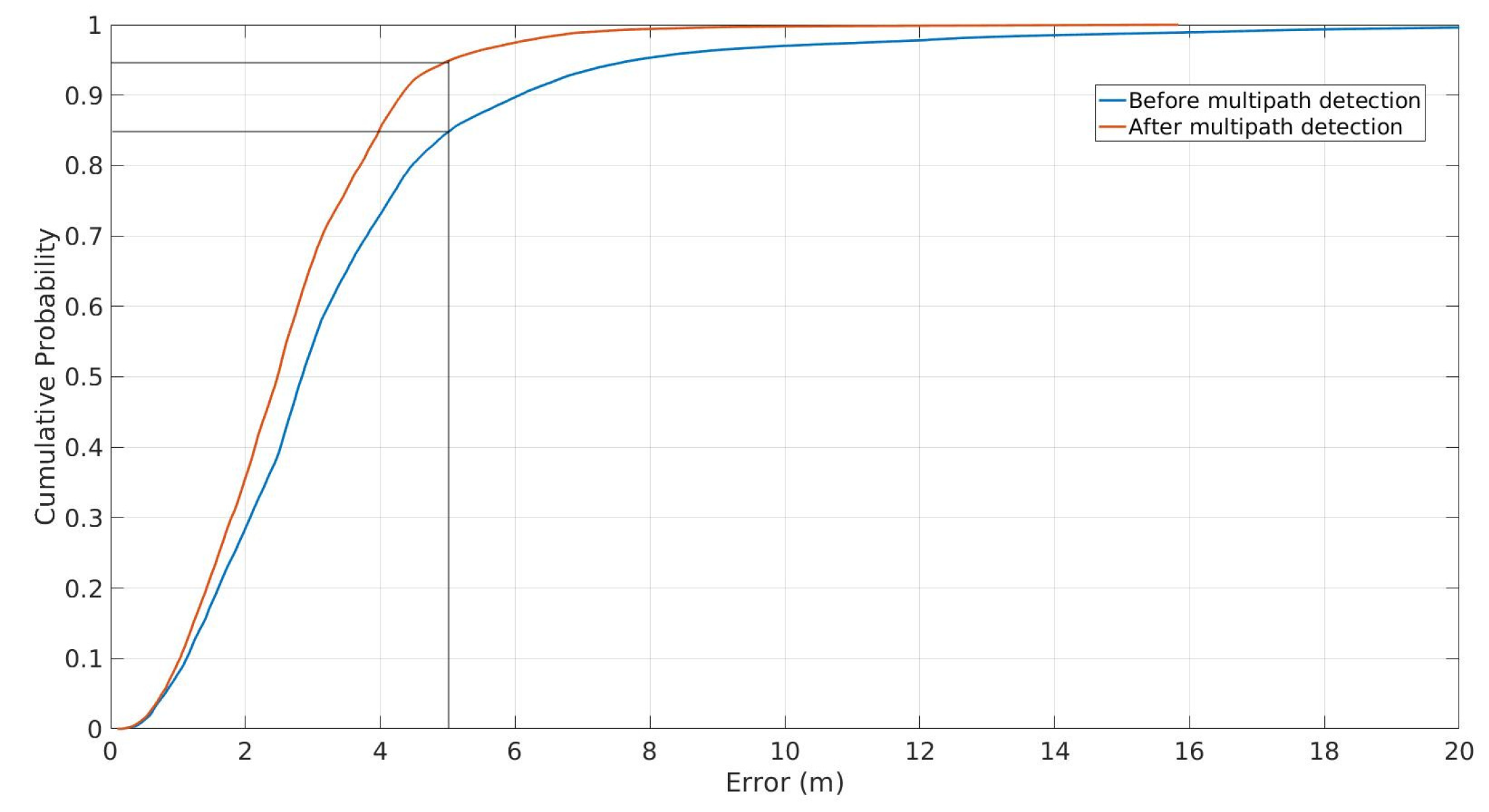
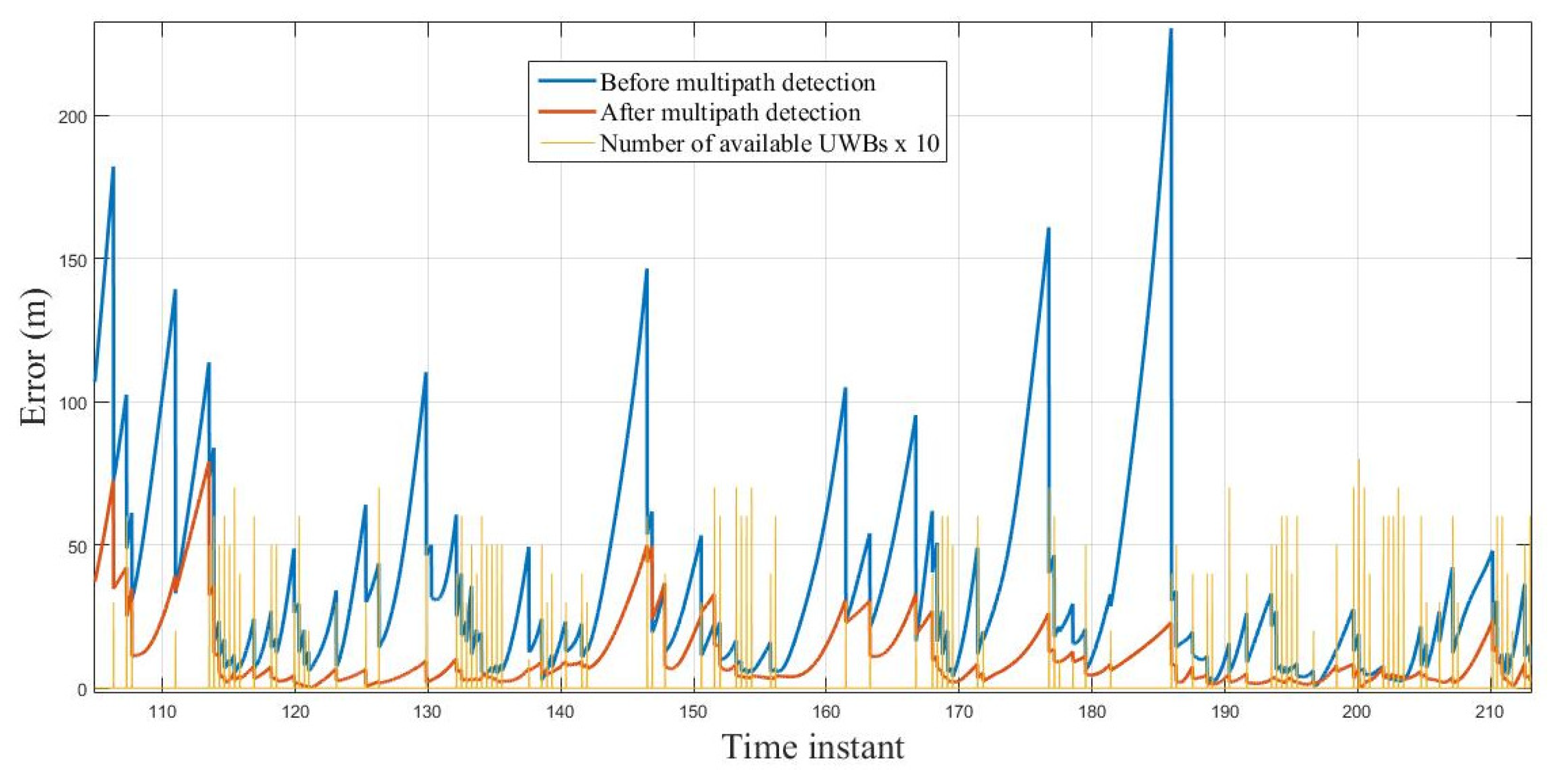
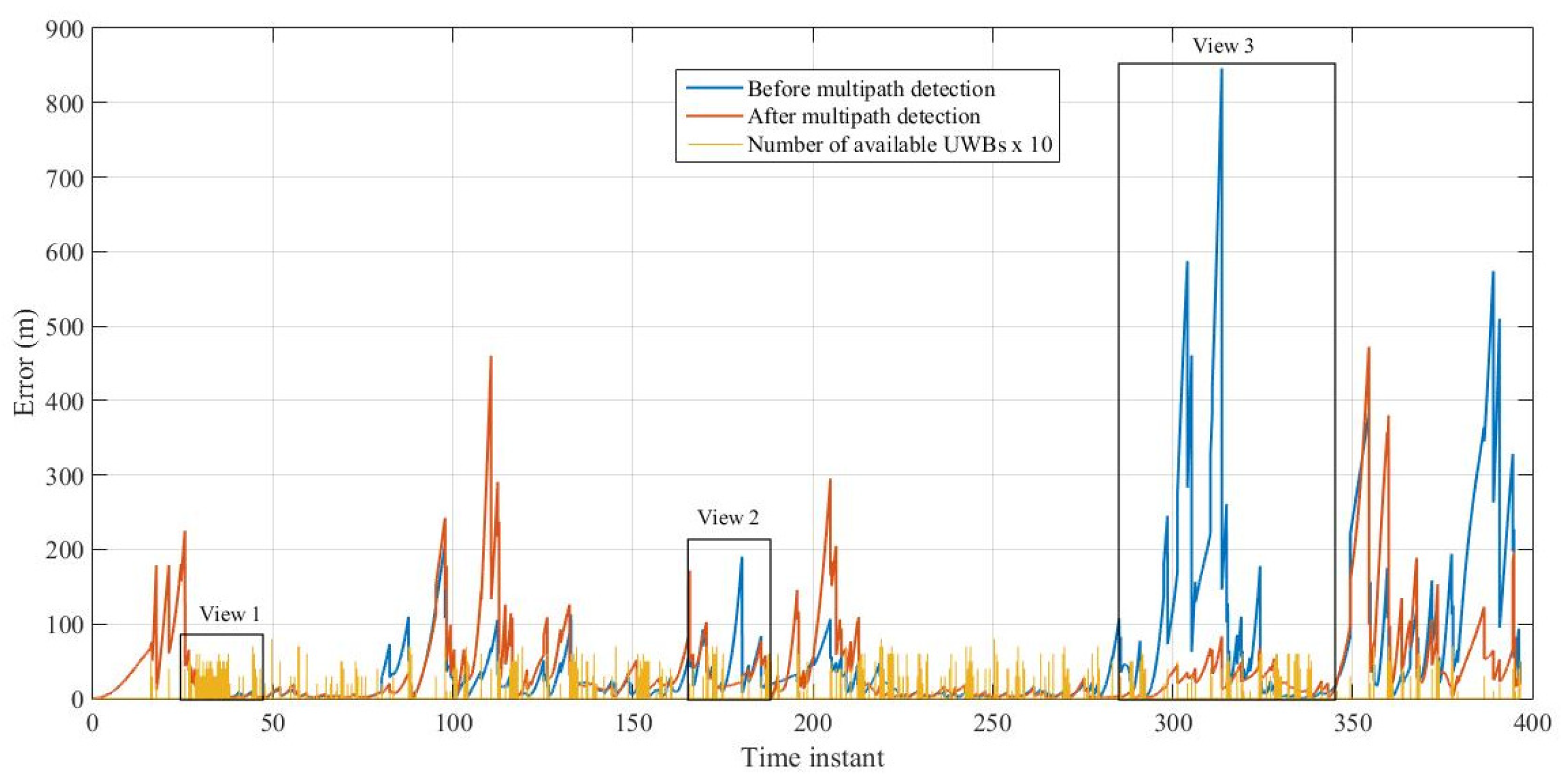
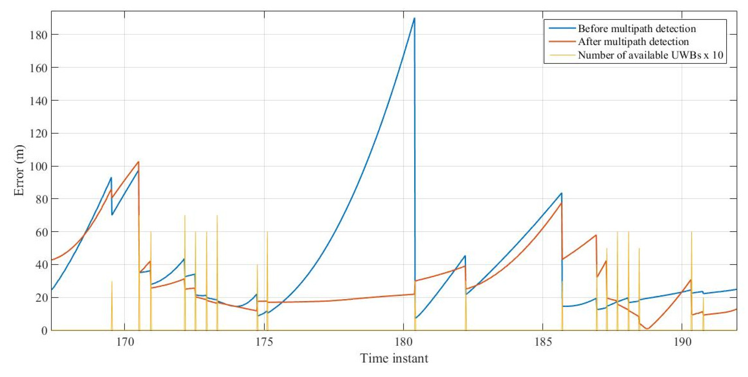
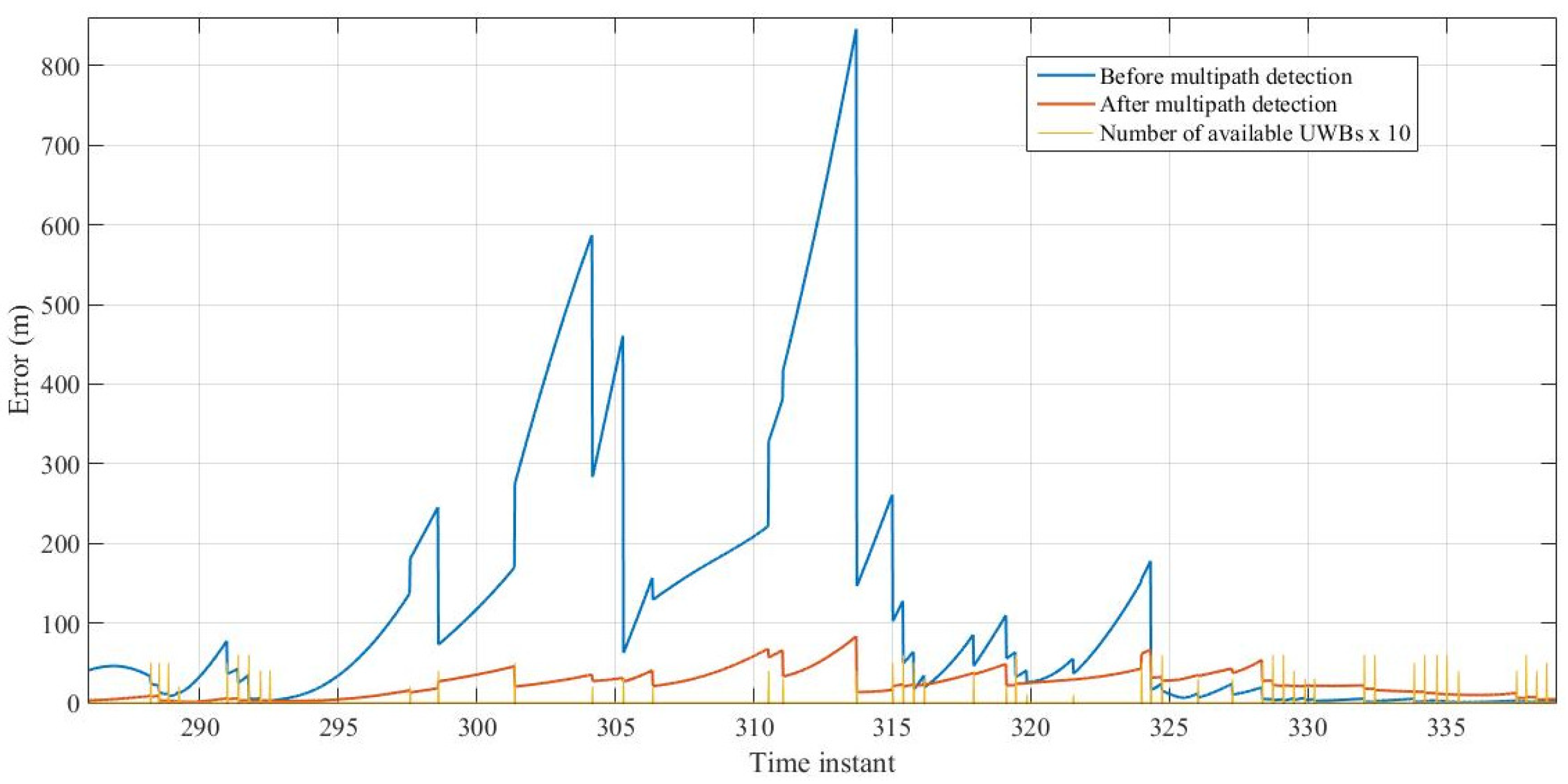
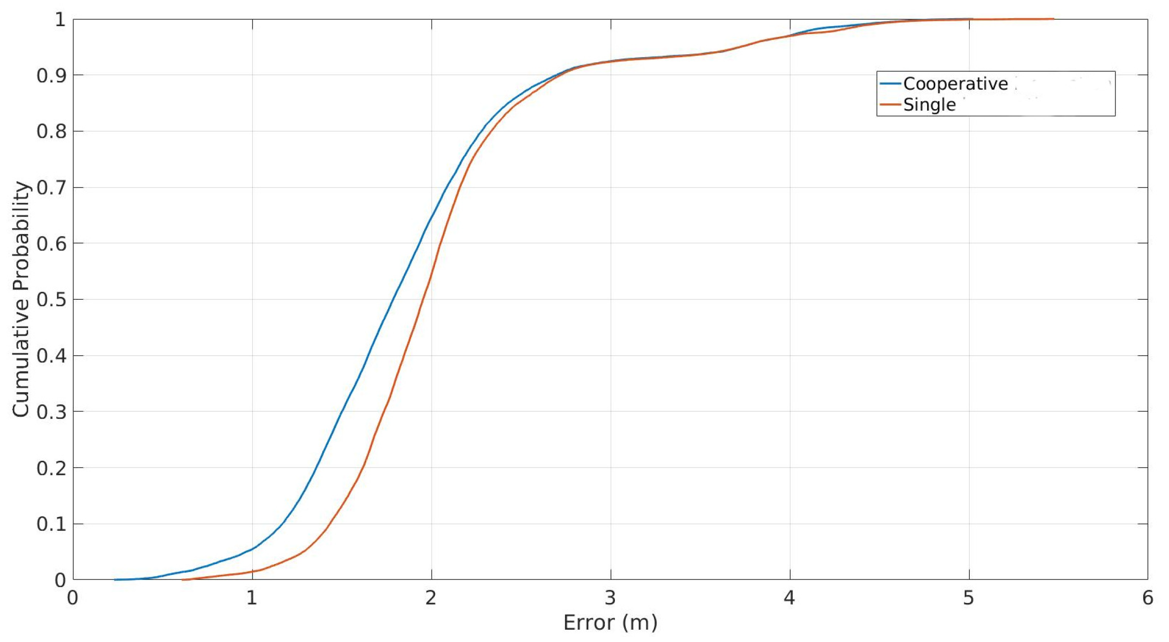
Table 1.
Details of sensors installed on the UAVs [12].
Table 1.
Details of sensors installed on the UAVs [12].
| Onboard Sensor | Dimension (L × W × H) | Weight (g) |
|---|---|---|
| uBlox GPS | 38 mm × 38 mm × 8.5 mm | 16.8 |
| P410 UWB | 76 mm × 80 mm × 16 mm | 58 |
| Raspberry Pi 3 | 85 mm × 56.5 mm | 45 |
| Pixhawk Autopilot | 81.5 mm × 50 mm × 15.5 mm | 38 |
| GoPro Camera | 60 mm × 42 mm × 30 mm | 74 |
Table 2.
Maximum size of joint measurement vector and matrix in a fully connected network.
| Measurement Type | Size of Vector | Size of Matrix |
|---|---|---|
| Pseudorange and relative range | ||
| Position and relative range | ||
| Relative range only | (or 16)N |
Table 3.
Accuracy evaluation of the UAV trajectory estimated using Photogrammetry.
| ID | Observed Error (all in m) | 3D error (in m) | ||
|---|---|---|---|---|
| Easting | Northing | Up | ||
| 1 | 0.006 | 0.011 | −0.008 | 0.014 |
| 3 | −0.002 | 0.015 | 0.008 | 0.017 |
| 8 | −0.018 | −0.002 | −0.019 | 0.026 |
| 9 | −0.019 | −0.004 | 0.008 | 0.021 |
| 11 | 0.007 | 0.002 | 0.003 | 0.008 |
| 17 | 0.019 | 0.021 | −0.018 | 0.034 |
| 18 | −0.008 | 0.018 | 0.005 | 0.021 |
| Overall 3D RMSE (m) | 0.022 | |||
Table 4.
Details of the experimental results presented in this section.
| Mode | Experiment Type | Operating Environment | |
|---|---|---|---|
| Infrastructure based Cooperative | Infrastructure based | GNSS denied | |
| P2P Cooperative | Centralized | Distributed | Partially GNSS denied |
| P2P Cooperative | Centralized | Full GNSS available | |
© 2018 by the authors. Licensee MDPI, Basel, Switzerland. This article is an open access article distributed under the terms and conditions of the Creative Commons Attribution (CC BY) license (http://creativecommons.org/licenses/by/4.0/).
Share and Cite
MDPI and ACS Style
Goel, S.; Kealy, A.; Lohani, B. Development and Experimental Evaluation of a Low-Cost Cooperative UAV Localization Network Prototype. J. Sens. Actuator Netw. 2018, 7, 42. https://doi.org/10.3390/jsan7040042
AMA Style
Goel S, Kealy A, Lohani B. Development and Experimental Evaluation of a Low-Cost Cooperative UAV Localization Network Prototype. Journal of Sensor and Actuator Networks. 2018; 7(4):42. https://doi.org/10.3390/jsan7040042
Chicago/Turabian StyleGoel, Salil, Allison Kealy, and Bharat Lohani. 2018. "Development and Experimental Evaluation of a Low-Cost Cooperative UAV Localization Network Prototype" Journal of Sensor and Actuator Networks 7, no. 4: 42. https://doi.org/10.3390/jsan7040042
Note that from the first issue of 2016, this journal uses article numbers instead of page numbers. See further details here.