1. Introduction
In recent years, there has been a great deal of work on the finite-sample properties of estimators and tests for linear regression models with endogenous regressors when the instruments are weak. Much of this work has focused on the case in which there is just one endogenous variable on the right-hand side, and numerous procedures for testing hypotheses about the coefficient of this variable have been studied. See, among many others, Staiger and Stock [
1], Stock, Wright, and Yogo [
2], Kleibergen [
3], Moreira [
4,
5], Andrews, Moreira, and Stock [
6], and Davidson and MacKinnon [
7,
8]. However, the closely related problem of testing overidentifying restrictions when the instruments are weak has been less studied. Staiger and Stock [
1] provides some asymptotic results, and Guggenberger, Kleibergen, Mavroeidis, and Chen [
9] derives certain asymptotic properties of tests for overidentifying restrictions in the context of hypotheses about the coefficients of a subset of right-hand side variables.
In the next section, we discuss the famous test of Sargan [
10] and other asymptotic tests for overidentification in linear regression models estimated by instrumental variables (IV) or limited information maximum likelihood (LIML). We show that the test statistics are all functions of six quadratic forms defined in terms of the two endogenous variables of the model, the linear span of the instruments, and its orthogonal complement. In fact, they can be expressed as functions of a certain ratio of sums of squared residuals and are closely related to the test proposed by Anderson and Rubin [
11]. In
Section 3, we analyze the properties of these overidentification test statistics. We use a simplified model with only three parameters, which is nonetheless capable of generating statistics with exactly the same distributions as those generated by a more general model, and characterize the finite-sample distributions of the test statistics, not by providing closed-form solutions, but by providing unique recipes for simulating them in terms of just eight mutually independent random variables with standard distributions as functions of the three parameters.
In
Section 4, we make use of these results in order to derive the limiting behavior of the statistics as the instrument strength tends to zero, as the correlation between the disturbances in the structural and reduced-form equations tends to unity, and as the sample size tends to infinity under the assumptions of weak-instrument asymptotics. Since the results of
Section 4 imply that none of the tests we study is robust with weak instruments,
Section 5 discusses a number of bootstrap procedures that can be used in conjunction with any of the overidentification tests. Some of these procedures are purely parametric, while others make use of resampling.
Then, in
Section 6, we investigate by simulation the finite-sample behavior of the statistics we consider. Simulation evidence and theoretical analysis concur in strongly preferring a variant of a likelihood-ratio test to the more conventional forms of Sargan test. In
Section 7, we look at the performance of bootstrap tests, finding that the best of them behave very well if the instruments are not too weak. However, as our theory suggests, they improve very little over tests based on asymptotic critical values in the neighborhood of the singularity that occurs where the instrument strength tends to zero and the correlation of the disturbances tends to one.
In
Section 8, we analyze the power properties of the two main variants of bootstrap test. We obtain analytical results that generalize those of
Section 3. Using those analytical results, we conduct extensive simulation experiments, mostly for cases that allow the bootstrap to yield reliable inference. We find that bootstrap tests based on IV estimation seem to have a slight power advantage over those based on LIML, at the cost of slightly greater size distortion under the null when the instruments are not too weak.
Section 9 presents a brief discussion of how both the test statistics and the bootstrap procedures can be modified to take account of heteroskedasticity and clustered data. Finally, some concluding remarks are made in
Section 10.
2. Tests for Overidentification
Although the tests for overidentification that we deal with are applicable to linear regression models with any number of endogenous right-hand side variables, we restrict attention in this paper to a model with just one such variable. We do so partly for expositional convenience and partly because this special case is of particular interest and has been the subject of much research in recent years. The model consists of just two equations,
Here
and
are
-vectors of observations on endogenous variables,
is an
matrix of observations on exogenous variables, and
is an
matrix of instruments such that
, where the notation
means the linear span of the columns of the matrix
. The disturbances are assumed to be homoskedastic and serially uncorrelated. We assume that
, so that the model is overidentified.
The parameters of this model are the scalar
β, the
-vector
γ, the
-vector
π, and the
contemporaneous covariance matrix of the disturbances
and
:
Equation (
1) is the structural equation we are interested in, and Equation (2) is a reduced-form equation for the second endogenous variable
.
The model (1) and (2) implicitly involves one identifying restriction, which cannot be tested, and
overidentifying restrictions. These restrictions say, in effect, that if we append
q regressors all belonging to
to Equation (
1) in such a way that the equation becomes just identified, then the coefficients of these
q additional regressors are zero.
The most common way to test the overidentifying restrictions is to use a Sargan test (Sargan, [
10]), which can be computed in various ways. The easiest is probably to estimate Equation (
1) by instrumental variables (IV), using the
l columns of
as instruments, so as to obtain the IV residuals
where
and
denote the IV estimates of
β and
γ, respectively. The IV residuals
are then regressed on
. The explained sum of squares from this regression divided by the IV estimate of
is the test statistic, and it is asymptotically distributed as
.
The numerator of the Sargan statistic can be written as
where
and
denote the IV estimates of
β and
γ, respectively, and
projects orthogonally onto
. We define
similarly, and let
and
. Since
is orthogonal to the IV residuals,
Then, since
, the numerator of the Sargan statistic can also be written as
Similarly, the denominator is just
In addition to being the numerator of the Sargan statistic, expression (
6) is the numerator of the Anderson-Rubin, or AR, statistic for the hypothesis that
; see Anderson and Rubin [
11]. The denominator of this same AR statistic is
which may be compared to the right-hand side of Equation (
7). We see that the Sargan statistic estimates
under the null hypothesis, and the AR statistic estimates it under the alternative.
Of course, AR statistics are usually calculated for the hypothesis that
β takes on a specific value, say
, rather than
. Since by definition
minimizes the numerator (
5), it follows that the numerator of the AR statistic is always no smaller than the numerator of the Sargan statistic. Even though the AR statistic is not generally thought of as a test of the overidentifying restrictions, it could be used as such a test, because it will always reject if the restrictions are sufficiently false, since that will cause the noncentrality parameter to be large.
It seems natural to modify the Sargan statistic by using (
8) instead of (
7) as the denominator, and this was done by Basmann [
12]. The usual Sargan statistic can be written as
and the Basmann statistic as
where
is the sum of squared residuals from regressing
on
,
is the SSR from regressing
on
, and
. Observe that both test statistics are simply monotonic functions of
, the ratio of the two sums of squared residuals.
Another widely used test statistic for overidentification is the likelihood ratio, or LR, statistic associated with the LIML estimate
. This statistic is simply
, where
The LIML estimator
minimizes
with respect to
β. Since
is just
, we see that the LR statistic is
. It is easy to show that, under both conventional and weak-instrument asymptotics, and under the null hypothesis,
as the sample size
n tends to infinity. Therefore, the LR statistic is asymptotically equivalent to the linearized likelihood ratio statistic
where
. We define LR
as
rather than as
by analogy with (
10). In what follows, it will be convenient to analyze LR
rather than LR.
We have seen that the Sargan statistic (
9), the Basmann statistic (
10), and the two likelihood ratio statistics LR and LR
are all monotonic functions of the ratio of SSRs
for some estimator
. Both the particular function of
that is used and the choice of
affect the finite-sample properties of an asymptotic test. For a bootstrap test, however, it is only the choice of
that matters. This follows from the fact that it is only the rank of the actual test statistic in the ordered list of the actual and bootstrap statistics that determines a bootstrap
P value; see
Section 6 below and Davidson and MacKinnon [
13]. Therefore, for any given bootstrap data-generating process (DGP) and any estimator
, bootstrap tests based on any monotonic transformation of
yield identical results.
3. Analysis Using a Simpler Model
It is clear from (
6), (
7), and (
11) that all the statistics we have considered for testing the overidentifying restrictions depend on
and
only through their projections
and
. We see also that
is homogeneous of degree zero with respect to
and
separately, for any
β. Thus the statistics depend on the scale of neither
nor
. Moreover, the matrix
plays no essential role. In fact, it can be shown—see Davidson and MacKinnon [
7],
Section 3—that the distributions of the test statistics generated by the model (1) and (2) for sample size
n are identical to those generated by the simpler model
where the sample size is now
, the matrix
has
columns, and
.
In the remainder of the paper, we deal exclusively with the simpler model (13) and (14). By doing so, we avoid the additional algebra made necessary by the presence of
in Equation (
1) without changing the results in any essential way. Of course,
,
, and
in the simpler model are not the same as in the original model, although
ρ is unchanged. For the original model,
n and
l in our results below would have to be replaced by
and
, and
and
would have to be replaced by
and
.
It is well known—see Mariano and Sawa [
14]—that all the test statistics depend on the data generated by (13) and (14) only through the six quadratic forms
This is also true for the general model (1) and (2), except that the projection matrix
must be replaced by
.
In this section and the next, we make the additional assumption that the disturbances
and
are normally distributed. Since the quadratic forms in (
15) depend on the instruments only through the projections
and
, it follows that their joint distribution depends on
only through the number of instruments
l and the norm of the vector
. We can therefore further simplify Equation (14) as
where the vector
is normalized to have length unity, which implies that
. Thus the joint distribution of the six quadratic forms depends only on the three parameters
β,
a, and
ρ, and on the dimensions
n and
l; for the general model (1) and (2), the latter would be
and
.
The above simplification was used in Davidson and MacKinnon [
7] in the context of tests of hypotheses about
β, and further details can be found there. The parameter
a determines the strength of the instruments. In weak-instrument asymptotics,
, while in conventional strong-instrument asymptotics,
. Thus, by treating
a as a parameter of order unity, we are in the context of weak-instrument asymptotics; see Staiger and Stock [
1]. The square of the parameter
a is often referred to as the (scalar) concentration parameter; see Phillips [
15] (p. 470), and Stock, Wright, and Yogo [
2].
Davidson and MacKinnon [
7] show that, under the assumption of normal disturbances, the six quadratic forms (
15) can be expressed as functions of the three parameters
β,
a, and
ρ and eight mutually independent random variables, the distributions of which do not depend on any of the parameters. Four of these random variables, which we denote by
,
,
, and
, are standard normal, and the other four, which we denote by
,
,
, and
, are respectively distributed as
,
,
, and
. In terms of these eight variables, we make the definitions
These quantities have simple interpretations:
, and
, for
.
Theorem 1. The Basmann statistic
defined in (
10) can be expressed as
and the statistic LR
defined in (
12) can be expressed as
where
with
, and
Remark 1. By substituting the relations (
20) and (
17) into (
18) and (
19), realizations of
and LR
can be generated as functions of realizations of the eight independent random variables. Since these have known distributions, it follows that Theorem 1 provides a complete characterization of the distributions of the statistics
and LR
in finite samples for arbitrary values of the parameters
β,
a, and
ρ. Although it seems to be impossible to obtain closed-form solutions for their distribution functions, it is of course possible to approximate them arbitrarily well by simulation.
4. Particular Cases
In this section, we show that no test of the overidentifying restrictions is robust to weak instruments. In fact, the distributions of and LR have a singularity at the point in the parameter space at which and , or, equivalently, . By letting for arbitrary values of a and r, we may obtain asymptotic results for both weak and strong instruments. In this way, we show that the singularity is present both in finite samples and under weak-instrument asymptotics. For conventional asymptotics, it is necessary to let both a and n tend to infinity, and in that case the singularity becomes irrelevant.
Like Theorem 1, the theorems in this section provide finite-sample results. Asymptotic results follow from these by letting the sample size n tend to infinity.
Theorem 2. When the parameter
a is zero, the linearized likelihood ratio statistic LR
, in terms of the random variables defined in (
17), is
where the discriminant Δ has become
independent of
r. When
, LR
is
independent of
a.
Remark 2.1. As with Theorem 1, the expressions (
21)–(
23) constitute a complete characterization of the distribution of LR
in the limits when
and when
.
Remark 2.2. The limiting value (
21) for
is independent of
r. Thus the distribution of LR
in the limit of completely irrelevant instruments is independent of all the model parameters.
Remark 2.3. The limiting value (
23) for
is independent of
a, and it tends to a
variable as
.
Remark 2.4. The singularity mentioned above is a consequence of the fact that the limit at is ill-defined, since LR converges to two different random variables as for and as for . These random variables are quite different and have quite different distributions.
Remark 2.5. Simulation results show that the limit to which LR converges as it approaches the singularity with for some positive α depends on α. In other words, the limit depends on the direction from which the singularity is reached.
Remark 2.6. The limit as
may appear to be of little interest. However, it may have a substantial impact on bootstrap inference. Davidson and MacKinnon [
7] show that
a and
r are not consistently estimated with weak instruments, and so, even if the true value of
r is far from zero, the estimate needed for the construction of a bootstrap DGP (see
Section 5) may be close to zero.
Remark 2.7. In the limit of strong instruments, the distribution of LR is the same as its distribution when , as shown by the following corollary.
Corollary 2.1. The limit of LR
as
, which is the limit when the instruments are strong, is
Proof of Corollary 2.1. Isolate the coefficients of powers of
a in (
19), and perform a Taylor expansion for small
. The result (
24) follows easily. ☐
As
,
, and so the result (
24) confirms that the asymptotic distribution with strong instruments is just
. In fact, Guggenberger
et al. [
9] demonstrate that, for our simple model, the asymptotic distribution is bounded by
however weak or strong the instruments may be. Some of the simulation results in
Section 6 for finite samples are in accord with this result.
Theorem 3. The Basmann statistic
in the limit with
becomes
where
The limit with
is
Proof. The proof is omitted. It involves tedious algebra similar to that in the proof of Theorem 2; see the
Appendix. ☐
Remark 3.1. The expression (
25) for
depends on
r, unlike the analogous expression for LR
. When
with
, it is easy to see that
tends to the limit
Remark 3.2. Similarly, the expression (
26) for
depends on
a. Its limit as
is
which is quite different from (
27), where the order of the limits is inverted. As with LR
, the limit as the singularity is approached depends on the direction of approach.
Remark 3.3. As expected, the limit of as is the same as that of LR.
The fact that the test statistics and LR depend on the parameters a and ρ indicates that these statistics are not robust to weak instruments. Passing to the limit as with weak-instrument asymptotics does not improve matters. Of the six quadratic forms on which everything depends, only the depend on n. Their limiting behavior is such that , , and as . In contrast, the do not depend on n, and they do depend on a and ρ.
5. Bootstrap Tests
Every test statistic has a distribution which depends on the DGP that generated the sample from which it is computed. The “true” DGP that generated an observed realization of the statistic is in general unknown. However, according to the bootstrap principle, one can perform inference by replacing the unknown DGP by an estimate of it, which is called the bootstrap DGP. Because what we need for inference is the distribution of the statistic under DGPs that satisfy the null hypothesis, the bootstrap DGP must necessarily impose the null. This requirement by itself does not lead to a unique bootstrap DGP, and we will see in this section that, for an overidentification test, there are several plausible choices.
If the observed value of a test statistic
τ is
, and the rejection region is in the upper tail, then the bootstrap
P value is the probability, under the bootstrap distribution of the statistic, that
τ is greater than
. To estimate this probability, one generates a large number, say
B, of realizations of the statistic using the bootstrap DGP. Let the
jth realization be denoted by
. Then the simulation-based estimate of the bootstrap
P value is just the proportion of the
greater than
:
where
is the indicator function, which is equal to 1 when its argument is true and 0 otherwise. If this fraction is smaller than
α, the level of the test, then we reject the null hypothesis. See Davidson and MacKinnon [
13].
5.1. Parametric Bootstraps
The DGPs contained in the simple model defined by Equation (
13) and Equation (
16) are characterized by just three parameters, namely,
β,
a, and
ρ. Since the value of
β does not affect the distribution of the overidentification test statistics (see Lemma 1 in the
Appendix), the bootstrap DGP for a parametric bootstrap (assuming normally distributed disturbances) is completely determined by the values of
a and
ρ that characterize it.
The test statistic itself may be any one of the overidentification statistics we have discussed. The model that is actually estimated in order to obtain is not the simple model, but rather the full model given by Equations (1) and (2). The parameters of this model include some whose values do not interest us for the purpose of defining a bootstrap DGP: β, since it has no effect on the distribution of the statistic, and γ, since the matrix plays no role in the simple model, from which the bootstrap DGP is taken. There remain π, ρ, , and .
For Equation (
16), the parameter
a was defined as the square root of
. However, this definition assumes that the vector
has unit length and that all the variables are scaled so that the variance of the disturbances
is 1. A more general definition of
a that does not depend on these assumptions is
It follows from (
29) that, in order to estimate
a, it is necessary also to estimate
.
Since the parameter
ρ is the correlation of the disturbances, which are not observed, any estimate of
ρ must be based on the residuals from the estimation of Equations (1) and (2). Let these residuals be denoted by
and
. Then the obvious estimators of the parameters of the covariance matrix are
and the obvious estimator of
a is given by
where
estimates
π. For
, there are two obvious choices, the IV residuals and the LIML residuals from (
1). For
, the obvious choice is the vector of OLS residuals from (2), possibly scaled by a factor of
to take account of the lost degrees of freedom in the OLS estimation. However, this obvious choice is not the only one, because, if we treat the model (1) and (2) as a system, the system estimator of
π that comes with the IV estimator of
β is the three-stage least squares (3SLS) estimator, and the one that comes with the LIML estimator of
β is the full-information maximum likelihood (FIML) estimator. These system estimators give rise to estimators not only of
π, but also of
, that differ from those given by OLS.
The system estimators of
π can be computed without actually performing a system estimation, by running the regression
see Davidson and MacKinnon [
7], where this matter is discussed in greater detail. If
is the vector of IV residuals, then the corresponding estimator
is the 3SLS estimator; if it is the vector of LIML residuals, then
is the FIML estimator.
For the purpose of computation, it is worth noting that all these estimators can be expressed as functions of the six quadratic forms (
15). A short calculation shows that the estimators of
and
ρ based on IV residuals, scaled OLS residuals, and the OLS estimator of
π are
where
is the difference between the IV estimator of
β and the true
β of the DGP, and where
From (
17), we can express
as
The weak-instrument asymptotic limit of this expression replaces the denominator divided by
by 1. The expectation of the numerator without the factor of
is
. Consequently, it may be preferable to reduce bias in the estimation of
by setting
; see Davidson and MacKinnon [
7].
The system estimator of the vector
π, which we write as
, is computed by running regression (
31). A tedious calculation shows that
with
where
is
and
is the vector of IV residuals if the structural Equation (
1) is estimated by IV, and
is
and
is the vector of LIML residuals if (
1) is estimated by LIML. Then, if
is estimated using the residuals
, we find that
Using the results (
33) and (
34) in (
30) allows us to write
For the parameter
ρ, more calculation shows that
We consider four different bootstrap DGPs. The simplest, which we call the IV-R bootstrap, uses the IV and OLS estimates of
a and
ρ given in (
32). The IV-ER bootstrap is based on 3SLS estimation of the two-equation system, that is, on IV estimation of (
1) and OLS estimation of regression (
31) with
the vector of IV residuals. Similarly, the LIML-ER bootstrap relies on FIML estimation of the system, that is, on LIML for (
1) and on regression (
31) with
the LIML residuals. Finally, we also define the F(1)-ER bootstrap, which is the same as LIML-ER except that
is replaced at every step by the modified LIML estimator of Fuller [
16] with
which is discussed in
Section 6.
It is plain that, the closer the bootstrap DGP is to the true DGP, the better will be bootstrap inference; see Davidson and MacKinnon [
17]. We may therefore expect that IV-ER should perform better than IV-R, and that LIML-ER should perform better than IV-ER. Between LIML-ER and F(1)-ER, there is no obvious reason
a priori to expect that one of them would outperform the other. But, whatever the properties of these bootstraps may be when the true DGP is not in the neighborhood of the singularity at
,
, we cannot expect anything better than some improvement over inference based on asymptotic critical values, rather than truly reliable inference, in the neighborhood of the singularity.
5.2. Resampling
Any parametric bootstrap risks being unreliable if the strong assumptions used to define the null hypothesis are violated. Most practitioners would therefore prefer a more robust bootstrap method. The strongest assumption we have made so far is that the disturbances are normally distributed. It is easy to relax this assumption by using a bootstrap DGP based on resampling, in which the bivariate normal distribution is replaced by the joint empirical distribution of the residuals. The discussion of the previous subsection makes it clear that several resampling bootstraps can be defined, depending on the choice of residuals that are resampled.
The most obvious resampling bootstrap DGP in the context of IV estimation is
where
and
are
-vectors of bootstrap observations,
and
are
-vectors of bootstrap disturbances with typical elements
and
, respectively, and
is the OLS estimate from Equation (2). The bootstrap disturbances are drawn in pairs from the bivariate empirical distribution of the structural residuals
and the rescaled reduced-form residuals
. That is,
Here EDF stands for “empirical distribution function”.
The rescaling of the reduced form residuals
in (
37) ensures that the distribution of the
has variance equal to the unbiased OLS variance estimator. The fact that the bootstrap disturbances are drawn in pairs ensures that the bootstrap DGP mimics the correlation between the two sets of residuals. Of course, whether that correlation consistently estimates the correlation between the actual disturbances depends on whether or not
can be estimated consistently. Under weak-instrument asymptotics,
cannot be estimated consistently; see Davidson and MacKinnon [
7].
Since all of the overidentification test statistics are invariant to the values of
β and
γ, we may replace the bootstrap DGP for
given by (
35) by
The bootstrap statistics generated by (38) and (36) are identical to those generated by (35) and (36). We will refer to the bootstrap DGP given by (36)–(38), as the IV-R resampling bootstrap. It is a semiparametric bootstrap, because it uses parameter estimates of the reduced-form equation, but it does not assume a specific functional form for the joint distribution of the disturbances. The empirical distribution of the residuals has a covariance matrix which is exactly that used to estimate
a and
ρ by the IV-R parametric bootstrap; hence our nomenclature.
The IV-ER resampling bootstrap draws pairs from the joint EDF of the IV residuals
from Equation (
1) and the residuals
computed by running regression (
31) with
replacing
. It also uses the resulting estimator
in (36) instead of the OLS estimator
. Note that the residuals
are
not the residuals from regression (
31), but rather those residuals plus
.
The LIML-ER resampling bootstrap is very similar to the IV-ER one, except that it uses
both directly and in regression (
31). Formally, the resampling procedure draws pairs from the bivariate empirical distribution of
Similarly, for the F(1)-ER resampling bootstrap, the structural Equation (
1) is estimated by Fuller’s method, and the residuals from this are used both for resampling and in regression (
31); see the next section.
A word of caution is advisable here. Although the values of overidentification test statistics are invariant to
β, thereby allowing us to use (
38) instead of (
35) in the bootstrap DGP, the residuals from which we resample in (
37) and (
39) do depend on the estimate of
β, as does the estimate of
π if it is based on any variant of Equation (
31). Nevertheless, the test statistics depend on the estimate of
β only through the residuals and the estimate of
π.
6. Performance of Asymptotic Tests: Simulation Results
The discussion in
Section 4 was limited to the statistics
and LR
. For bootstrap tests, it is enough to consider just these two, since all other statistics mentioned in
Section 2 are monotonic transforms of them. Of course, the different versions of the Sargan test and the LR test have different properties when used with (strong-instrument) asymptotic critical values. In this section, we therefore present some Monte Carlo results on the finite-sample performance of five test statistics, including
S,
, LR, and LR
.
The fifth test statistic we examine is based on the estimator proposed by Fuller [
16]. Like the IV and LIML estimators, Fuller’s estimator is a
K-class estimator for model (1) and (2). It takes the form
Setting
, the minimized value of the variance ratio (
11), in Equation (
40) gives the LIML estimator, while setting
gives the IV estimator. Fuller’s estimator sets
for some fixed number
independent of the sample size
n. We set
. With this choice, Fuller’s estimator
has all moments (except when the sample size is very small) and is approximately unbiased. The corresponding test statistic is simply
, which has the same form as the LR statistic. We will refer to this as the LRF test.
The DGPs used for our simulations all belong to the simplified model (
13) and (
16). The disturbances are generated according to the relations
where
and
are
-vectors with independent standard normal elements, and
. Of course, it is quite unnecessary to generate simulated samples of
n observations, as it is enough to generate the six quadratic forms (
15) as functions of eight mutually independent random variables, using the relations (
17) and (
20). The sample size
n affects only the degrees of freedom of the two
random variables
and
that appear in (
17). Although any DGP given by (
13) and (
16) involves no explicit overidentifying restrictions, the test statistics are computed for the model (1) and (2), for which there are
of them, with
in the experiments.
The first group of experiments is intended to provide guidance on the appropriate sample size to use in the remaining experiments. Our objective is to mimic the common situation in which the sample size is reasonably large and the instruments are quite weak. Since our simulation DGPs embody weak-instrument asymptotics, we should not expect any of the test statistics to have the correct size asymptotically. However, for any given
a and
ρ, the rejection frequency converges as
to that given by the asymptotic distribution of the statistic used; these asymptotic distributions were discussed at the end of
Section 4. In the experiments, we use sample sizes of 20, 28, 40, 56, and so on, up to 1810. Each of these numbers is larger than its predecessor by approximately
. Each experiment used
replications.
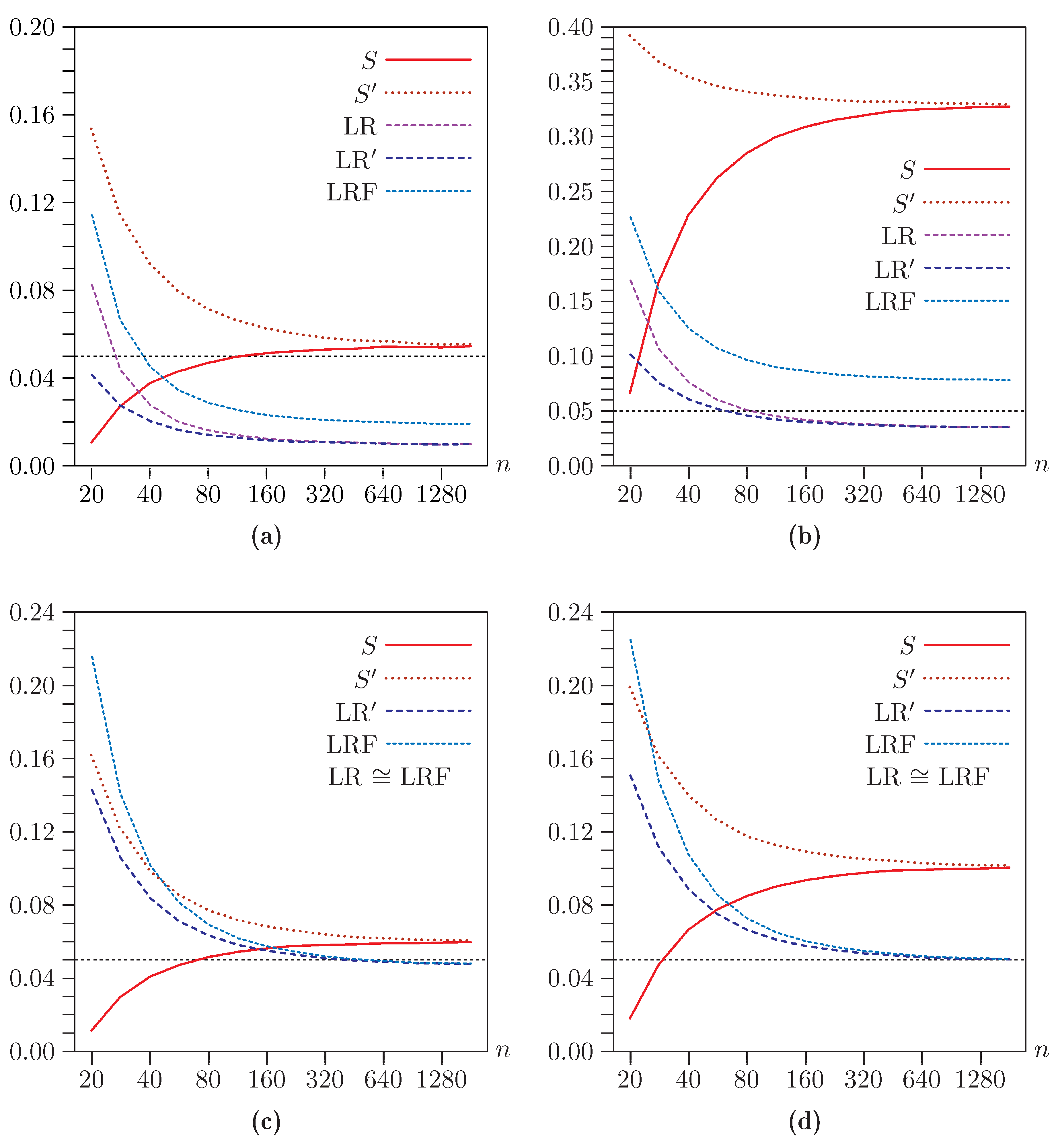
The results of four sets of experiments are presented in
Figure 1, in which we plot rejection frequencies in the experiments for a nominal level of 5%. In the top two panels,
, so that the instruments are very weak. In the bottom two panels,
, so that they are reasonably strong. Recall that the concentration parameter is
. In the two panels on the left,
, so that there is moderate correlation between the structural and reduced form disturbances. In the two panels on the right,
, so that there is strong correlation. Note that the vertical axis differs across most of the panels.
Figure 1.
Rejection frequencies for asymptotic tests as functions of n for . (a) , ; (b) , ; (c) , ; (d) , . Note that the scale of the vertical axis differs across panels.
Figure 1.
Rejection frequencies for asymptotic tests as functions of n for . (a) , ; (b) , ; (c) , ; (d) , . Note that the scale of the vertical axis differs across panels.
It is evident that the various asymptotic tests can perform very differently and that their performance varies greatly with the sample size. The Basmann test
always rejects more often than LR
. This must be the case, because the two test statistics are exactly the same function of
ζ—compare Equation (
10) and Equation (
12)—but the LIML estimator minimizes
and the IV estimator does not. Thus
must be closer to unity than
.
The Sargan (
S) and Basmann (
) tests perform almost the same for large samples but very differently for small ones, with the latter much more prone to overreject than the former. This could have been predicted from Equation (
9) and Equation (
10). If it were not for the different factors of
n and
,
would always be greater than
S, because
. For
, the difference between
and
is
. Therefore, under the null hypothesis, the difference between the two test statistics is
. This explains their rapid convergence as
n increases.
For , the LR test and its linearized version LR perform somewhat differently in small samples but almost identically once , with LR rejecting more often than LR. The difference between the two LIML-based statistics is much smaller than the difference between the two IV-based statistics for two reasons. First, because the LIML estimator minimizes , the two LR test statistics are being evaluated at values of ζ that are closer to unity than the two IV-based statistics. Second, is almost exactly half the magnitude of . Based on the fact that , we might expect LR to reject more often than LR. However, the difference between and n evidently more than offsets this, at least for , the case in the figure.
In this case, the Fuller variant of the LR test performs somewhat differently from both LR and LR for all sample sizes. In contrast, for , LR and LRF are so similar that we did not graph LR to avoid making the figure unreadable. LR, LR, and LRF perform almost identically, and very well indeed, for large sample sizes, even though they overreject severely for small sample sizes.
As expected, all of the rejection frequencies seem to be converging to constants as . Moreover, in every case, it appears that the (interpolated) results for are very similar to the results for larger values up to . Accordingly, we used in all the remaining experiments.
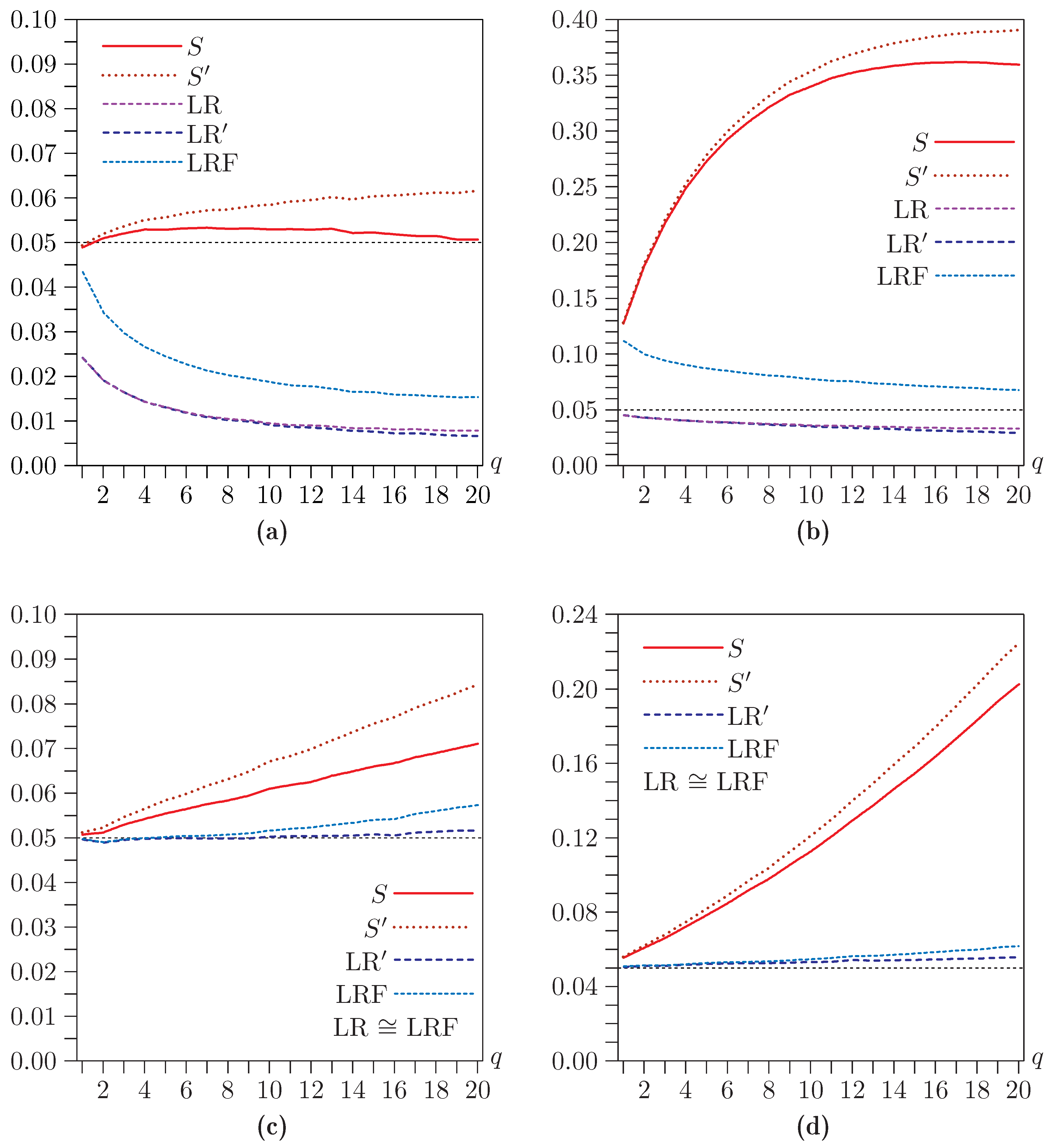
In the second group of experiments, the number of overidentifying restrictions
q is varied. The four panels in
Figure 2 correspond to those of
Figure 1. In most cases, performance deteriorates as
q increases. Sometimes, rejection frequencies seem to be converging, but by no means always. In the remaining experiments, we somewhat arbitrarily set
. Choosing a smaller number would generally have resulted in smaller size distortions.
In the third group of experiments, the results of which are shown in
Figure 3, we set
and
, and we vary
ρ between 0.0 and 0.99 at intervals of 0.01 for four values of
a. The vertical axis is different in each of the four panels, because the tests all perform much better as
a increases. For clarity, rejection frequencies for LR are not shown in the figure, because they always lie between those for LR
and LRF. They are very close to those for LR
when
a is small, and they are very close to those for LRF when
a is large.
For the smaller values of
a, all of the tests can either overreject or underreject, with rejection frequencies increasing in
ρ. The Sargan and Basmann tests overreject very severely when
a is small and
ρ is large. The LR
, LR, and LRF tests underreject severely when
a is small and
ρ is not large, but they overreject slightly when
a is large. Based on
Figure 1 and on the analysis of the previous section, we expect that this slight overrejection vanishes for larger samples.
Figure 2.
Rejection frequencies for asymptotic tests as functions of q for . (a) , ; (b) , ; (c) , ; (d) , . Note that the scale of the vertical axis differs across panels.
Figure 2.
Rejection frequencies for asymptotic tests as functions of q for . (a) , ; (b) , ; (c) , ; (d) , . Note that the scale of the vertical axis differs across panels.
Figure 3.
Rejection frequencies for asymptotic tests as functions of ρ for and . (a) Very weak instruments: ; (b) Weak instruments: ; (c) Moderately strong instruments: ; (d) Very strong instruments: . Note that the scale of the vertical axis differs across panels.
Figure 3.
Rejection frequencies for asymptotic tests as functions of ρ for and . (a) Very weak instruments: ; (b) Weak instruments: ; (c) Moderately strong instruments: ; (d) Very strong instruments: . Note that the scale of the vertical axis differs across panels.
Although the performance of all the overidentification tests is quite poor when
a is small, it is worth noting that the Sargan tests are not as unreliable as
t tests of the hypothesis that
β has a specific value, and the LR tests for overidentification are not as unreliable as LR tests for that hypothesis; see Davidson and MacKinnon [
7,
8].
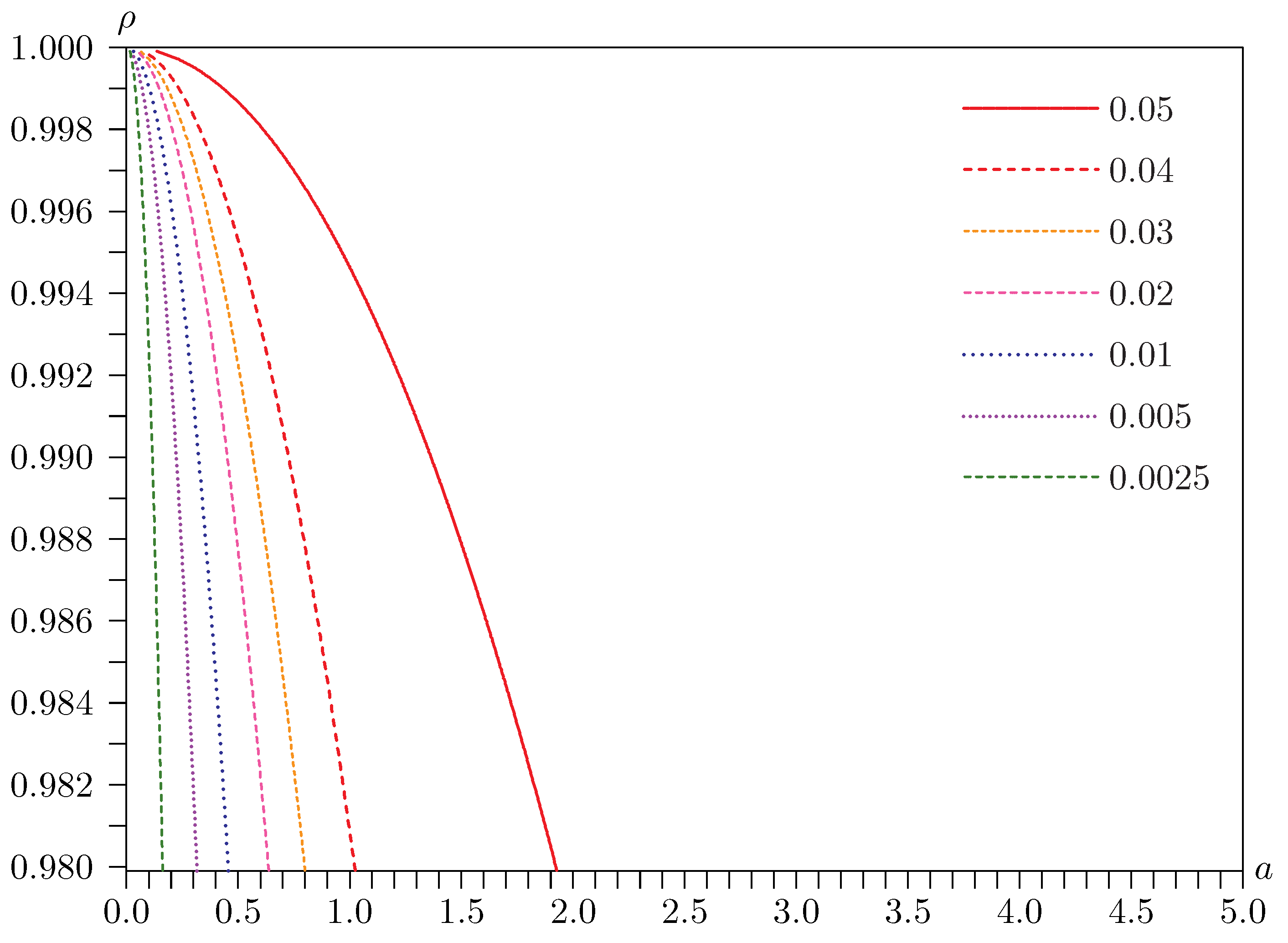
6.1. Near the Singularity
From
Figure 1,
Figure 2 and
Figure 3, we see that the rejection probabilities of all the tests vary considerably with the parameters
a and
ρ as they vary in the neighborhood of the singularity at
,
. Further insight into this phenomenon is provided by
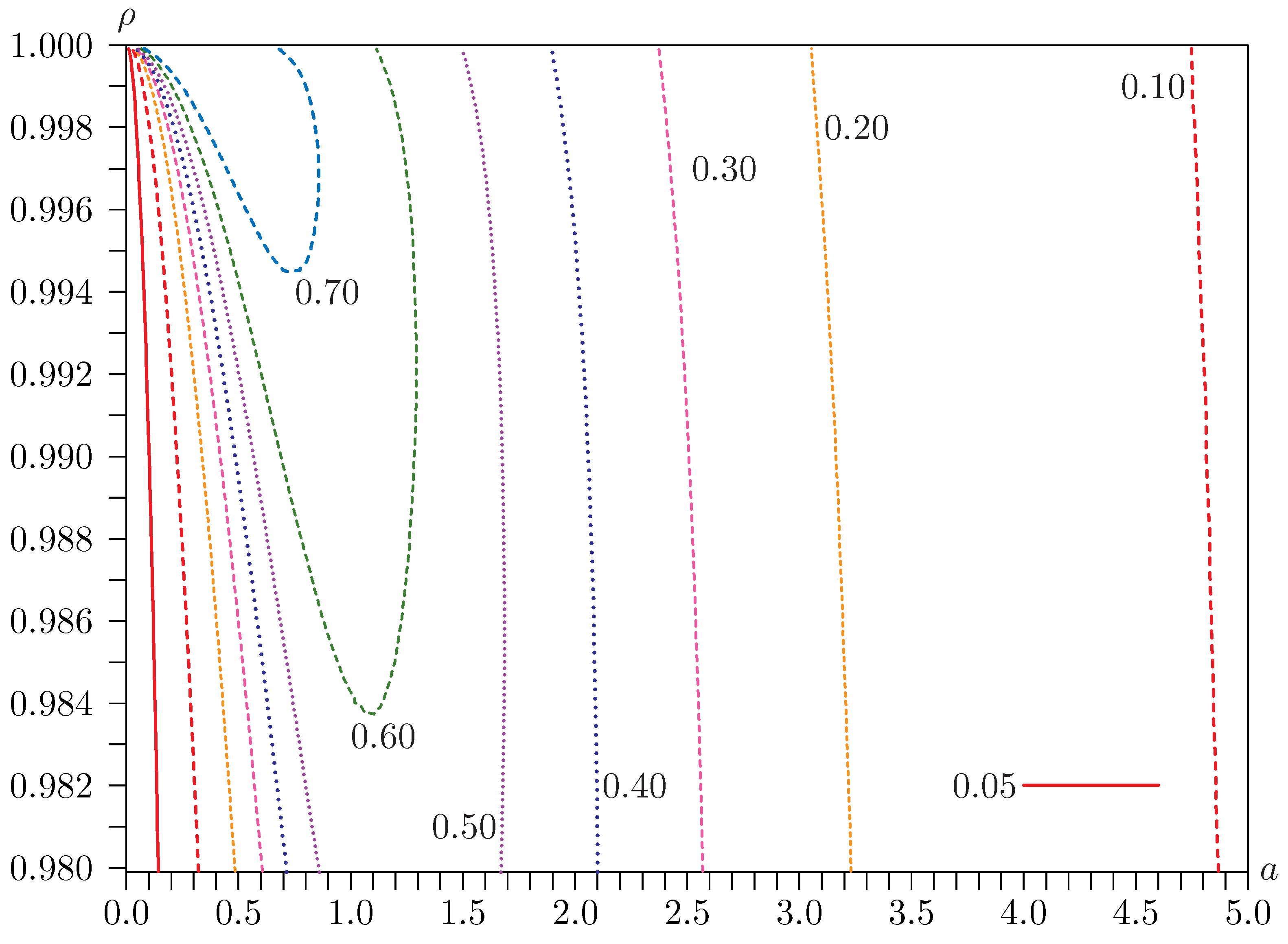
Figure 4 and
Figure 5. These are contour plots of rejection frequencies near the singularity for tests at the 0.05 level with
a and
ρ on the horizontal and vertical axes, respectively.
Figure 4 is for the Basmann statistic
, and
Figure 5 is for the LR
statistic. Both figures are for the case dealt with in
Figure 3, for which
and
. The rejection frequencies are, once again, estimated using
replications.
Figure 4.
Contours of rejection frequencies for tests with and .
Figure 4.
Contours of rejection frequencies for tests with and .
Figure 5.
Contours of rejection frequencies for likelihood ratio (LR) tests with and .
Figure 5.
Contours of rejection frequencies for likelihood ratio (LR) tests with and .
It is clear from these figures that rejection frequencies tend to be greatest as the singularity is approached by first setting
and then letting
a tend to zero. In this limit,
is given by expression (
28), and LR
is given by expression (
23). For extremely small values of
a,
actually underrejects. But, as
a rises to values that are still very very small, rejection frequencies soar, sometimes to over 0.80. In contrast, LR
underrejects severely for small values of
a, values which do not have to be nearly as small as in the case of
. In much of the figure, however, the rejection frequencies for LR
are just a little greater than 0.05.
The 95% quantile of the distribution of expression (
28) has the huge value of 16,285, as estimated from 9,999,999 independent realizations. In contrast, recall that the 95% quantile of the
distribution for
is 15.5073. Since the distribution of
for arbitrary
a and
ρ is stochastically bounded by that of (
28),
is boundedly pivotal. However, basing inference on the distribution of (
28) is certain to be
extremely conservative.
7. Performance of Bootstrap Tests
In principle, any of the bootstrap DGPs discussed in the previous section can be combined with any of the test statistics discussed in
Section 2. However, there is no point considering both
S and
, or both LR and LR
, because in each case one test statistic is simply a monotonic transformation of the other. If both the statistics in each pair are bootstrapped using the same bootstrap DGP, they must therefore yield identical results.
All of our experiments involve 100,000 replications for each set of parameter values, and the bootstrap tests mostly use . This is a smaller number than should generally be used in practice, but it is perfectly satisfactory for simulation experiments, because experimental randomness in the bootstrap p values tends to average out across replications. Although the disturbances of the true DGPs are taken to be normally distributed, the bootstrap DGPs we investigate in the main experiments are resampling ones, because we believe they are the ones that will be used in practice.
Figure 6,
Figure 7 and
Figure 8 present the results of a large number of Monte Carlo experiments.
Figure 6 concerns Sargan tests,
Figure 7 concerns LR tests, and
Figure 8 concerns Fuller LR tests. Each of the figures shows rejection frequencies as a function of
ρ for 34 values of
ρ, namely, 0.00, 0.03, 0.06,
…, 0.99. The four panels correspond to
, 4, 6, and 8. Note that the scale of the vertical axis often differs across panels within each figure and across figures for panels corresponding to the same value of
a. It is important to keep this in mind when interpreting the results.
As we have already seen, for small and moderate values of
a, Sargan tests tend to overreject severely when
ρ is large and to underreject modestly when it is small. It is evident from
Figure 6 that, for
, using either the IV-R or IV-ER bootstrap improves matters only slightly. However, both these methods do provide a more and more noticeable improvement as
a increases. For
, the improvement is very substantial. If we were increasing
n as well as
a, it would be natural to see this as evidence of an asymptotic refinement.
Figure 6.
Rejection frequencies for Sargan tests as functions of ρ for and . (a) ; (b) ; (c) ; (d) . Note that the scale of the vertical axis differs across panels.
Figure 6.
Rejection frequencies for Sargan tests as functions of ρ for and . (a) ; (b) ; (c) ; (d) . Note that the scale of the vertical axis differs across panels.
There seems to be no advantage to using IV-ER rather than IV-R. In fact, the latter always works a bit better when
ρ is very large. This result is surprising in the light of the findings of Davidson and MacKinnon [
7,
8] for bootstrapping
t tests on
β. However, the bootstrap methods considered in those papers imposed the null hypothesis that
, while the ones considered here do not. Apparently, this makes a difference.
Using the LIML-ER and F(1)-ER bootstraps with the Sargan statistic yields entirely different results. The former underrejects very severely for all values of ρ when a is small, but the extent of the underrejection drops rapidly as a increases. The latter always underrejects less severely than LIML-ER (it actually overrejects for large values of ρ when ), and it performs surprisingly well for . Of course, it may seem a bit strange to bootstrap a test statistic based on IV estimation using a bootstrap DGP based on LIML or its Fuller variant.
Figure 7.
Rejection frequencies for LR tests as functions of ρ for and . (a) ; (b) ; (c) ; (d) . Note that the scale of the vertical axis differs across panels.
Figure 7.
Rejection frequencies for LR tests as functions of ρ for and . (a) ; (b) ; (c) ; (d) . Note that the scale of the vertical axis differs across panels.
In
Figure 7, we see that, in contrast to the Sargan test, the LR test generally underrejects, often very severely when both
ρ and
a are small. Its performance improves rapidly as
a increases, however, and it actually overrejects slightly when
ρ and
a are both large. All of the bootstrap methods improve matters, and the extent of the improvement increases with
a. For
, all the bootstrap methods work essentially perfectly. For small values of
a, the IV-R bootstrap actually seems to be the best in many cases, although it does lead to modest overrejection when
ρ is large.
Figure 8.
Rejection frequencies for Fuller LR tests as functions of ρ for and . (a) ; (b) ; (c) ; (d) . Note that the scale of the vertical axis differs across panels.
Figure 8.
Rejection frequencies for Fuller LR tests as functions of ρ for and . (a) ; (b) ; (c) ; (d) . Note that the scale of the vertical axis differs across panels.
In
Figure 8, we see that the Fuller LR test never underrejects as much as the LR test, and it actually overrejects quite severely when
ρ is large and
. However, that is the only case in which it overrejects much. This is the only test for which its own bootstrap DGP, namely, F(1)-ER, is arguably the best one to use. Except when the asymptotic test already works perfectly, using that bootstrap method almost always improves the performance of the test. The bottom two panels of
Figure 8 look very similar to the corresponding panels of
Figure 7, except that the bootstrapped Fuller test tends to underreject just a bit. It is evident that, as
a increases, the LR test and its Fuller variant become almost indistinguishable.
Figure 6,
Figure 7 and
Figure 8 provide no clear ranking of tests and bootstrap methods. There seems to be a preference for the LR and Fuller LR tests, and for the LIML-ER and F(1)-ER bootstrap DGPs. In no case does any combination of those tests and those bootstrap DGPs overreject anything like as severely as the Sargan test bootstrapped using IV-R or IV-ER. Provided the instruments are not very weak, any of these combinations should yield reasonably accurate, but perhaps somewhat conservative, inferences in most cases.
The rather mixed performance of the bootstrap tests can be understood by using the concept of “bootstrap discrepancy,” which is a function of the nominal level of the test, say
α. The bootstrap discrepancy is simply the actual rejection rate for a bootstrap test at level
α minus
α itself. Davidson and MacKinnon [
18] shows that the bootstrap discrepancy at level
α is a conditional expectation of the random variable
where
is the probability, under the DGP
μ, that the test statistic is in the rejection region for nominal level
α, and
is the inverse function that satisfies the equation
Thus
is the true level-
α critical value of the asymptotic test under
μ. The random element in (
41) is
, the bootstrap DGP. If
, then we see clearly that
, and the bootstrap discrepancy vanishes. For more detail, see Davidson and MacKinnon [
18].
Figure 9.
Contours of rejection frequencies for instrumental variables (IV)-R bootstrap Sargan tests.
Figure 9.
Contours of rejection frequencies for instrumental variables (IV)-R bootstrap Sargan tests.
Suppose now that the true DGP
is near the singularity. The bootstrap DGP can reasonably be expected also to be near the singularity, but most realizations are likely to be farther away from the singularity than
itself. If
were actually at the singularity, then any bootstrap DGP would necessarily be farther away. If the statistic used is
S, then we see from
Figure 4 that rejection frequencies fall as the DGP moves away from the singularity in most, but not all, directions. Thus, for most such bootstrap DGPs,
is smaller than
for any
α, and so the probability mass
in the distribution generated by
is greater than
α. This means that
is positive, and so the bootstrap test overrejects. However, if the statistic used is LR, the reverse is the case, as we see from
Figure 5, and the bootstrap test underrejects. This is just what we see in
Figure 6,
Figure 7 and
Figure 8.
Figure 9 and
Figure 10 are contour plots similar to
Figure 4 and
Figure 5, but they are for bootstrap rather than asymptotic tests. The IV-R parametric bootstrap is used for the Sargan test in
Figure 9, and the LIML-ER parametric bootstrap is used for the LR test in
Figure 10. In both cases, there are 100,000 replications, and
.
Figure 9 looks remarkably like
Figure 4, with low rejection frequencies for extremely small values of
a, then a ridge where rejection frequencies are very high for slightly larger values of
a. The ridge is not quite as high as the one in
Figure 4, and the rejection frequencies diminish more rapidly as
a increases.
Figure 10.
Contours of rejection frequencies for limited information maximum likelihood (LIML)-ER bootstrap LR tests.
Figure 10.
Contours of rejection frequencies for limited information maximum likelihood (LIML)-ER bootstrap LR tests.
Similarly,
Figure 10 looks like
Figure 5, but the severe underrejection in the far left of the figure occurs over an even smaller region, and there is an area of modest overrejection nearby. Both these size distortions can be explained by
Figure 5. When
a is extremely small, the estimate used by the bootstrap DGP tends on average to be larger, so the bootstrap critical values tend, on average, to be overestimates. This leads to underrejection. However, there is a region where
a is not quite so small in which the bootstrap DGP uses estimates of
a that are sometimes too small and sometimes too large. The former causes overrejection, the latter underrejection. Because of the curvature of the rejection probability function, the net effect is modest overrejection; see Davidson and MacKinnon [
17]. This is actually the case for most of the parameter values shown in the figure, but the rejection frequencies are generally not much greater than 0.05.
8. Power Considerations
Overidentification tests are performed in order to check whether some of the assumptions for the two-equation model (1) and (2) to be correctly specified are valid. Those assumptions are not valid if the DGP for Equation (
1) is actually
where the columns of the matrix
are in the span of the columns of the matrix
and are linearly independent of those of
. As in
Section 3, we can eliminate
from the model, replacing all other variables and the disturbances by their projections onto the orthogonal complement of the span of the columns of
. The simpler model of Equation (
13) and Equation (
16) becomes
The vector
is now written as
instead of
, and the vector
is written as
. As before, we make the normalizations that
and
. In addition, we normalize so that
and
.
The disturbance vector
of (
13) is written as
. In the rightmost expression of Equations (44), the vector
has been replaced by
, where
. Since we are assuming, as in
Section 3, that the disturbance vectors
and
are normally distributed, the vectors
and
are independent
. Further, since
and
are not in general orthogonal, we write
where
, and
.
The Basmann statistic
is still given by Equation (
18), which is simply an algebraic consequence of the definition (
10). Since the DGP for
is unchanged, the quantities denoted in (
10) by
and
are the same under the alternative as under the null. Since the DGP for
is also the same under the null and the alternative, so are
and
. Thus only
and
differ from the expressions for them in Equations (
20). It is easy to check that neither the numerator nor the denominator of
in (
18) depends on
β under the alternative, and so in our computations we set
without loss of generality.
In order to analyze the asymptotic power of the Sargan test in Basmann form, we seek to express its limiting asymptotic distribution as a chi-squared variable that is non-central under the alternative. As usual, in order for the non-centrality parameter (NCP) to have a finite limit, we invoke a Pitman drift. With our normalization of , this just means that δ is constant as the sample size n tends to infinity. Again, we cannot expect to find a limiting chi-squared distribution with weak-instrument asymptotics, and so our asymptotic construction supposes that as .
Under the null and the alternative, the denominator of (
18), divided by
, is simply an estimate of the variance of
. For the purposes of the asymptotic analysis of the simpler model, it can therefore be replaced by 1. The quantity of which the limiting distribution is expected to be chi-squared is therefore
. Recall that this is just the numerator of both the
S and
statistics.
With
, we compute as follows:
where the symbol
means of order unity as
. As before, we let
for
, and we also let
. Thus the limit as
of
is
In Equation (
17), we introduced the quantity
, equal to
and distributed as
. It was expressed as the sum of three mutually independent random variables,
,
, and
. Now we separate out both the terms
and
to obtain
where all four random variables above are independent, with
,
, and
standard normal, and
distributed as
. The random variable
is not to be confused with
in Equations (
17), which is distributed as
. It is legitimate to write
in this way because it can be constructed as the sum of the squares of the
l independent
N(0,1) variables
, where the
form an arbitrary orthonormal basis of the span of the columns of
.
Using (
46), the right-hand side of Equation (
45) can be written as
This is the sum of three independent random variables. The first is
, the second is
, and the last is noncentral
. It follows that, when
and the sample size both tend to infinity, which implies that the instruments are not weak, the numerator of the test statistic is distributed as
. Note that, if
, so that
, the NCP
vanishes.
For the general model (1) and (2), with DGP given by Equation (
42), it can be shown that the NCP is
For the simpler model given by Equations (43) and (44), the first term here collapses to
and the second term, which arises because
β has to be estimated, collapses to
. Therefore, expression (
47) as a whole corresponds to
for the simpler model.
8.1. Finite-Sample Concerns
The asymptotic result that
follows the
distribution strongly suggests that
S, LR, and LR
must do so as well, because all these statistics are asymptotically equivalent. In fact, a more tedious calculation than that in Equation (
45) and Equation (
46) shows that the limiting distribution of
as both
n and
a tend to infinity is the same as for
, namely
. Because these results are only asymptotic, however, it is necessary to resort to simulation to investigate behavior under the alternative in finite samples.
Under the null, we were able in
Section 3 to express all six quantities, the
and the
, for
, in terms of eight independent random variables. Under the alternative, we require ten of these variables. For the
, there is no need to change the expressions for them in (
20), where we use the three variables
,
, and
, distributed respectively as
,
, and
N(0,1). These represent the projections of
and
onto the orthogonal complement of the span of the instruments. For the
, however, we decompose as follows:
Here
,
,
, and
are standard normal,
is
, and
is
, all seven variables being mutually independent. We can simulate both
and LR
very cheaply, by drawing ten random variables, independently of either the sample size
n or the degree of overidentification
, because all the statistics are deterministic functions of the
and the
, and, of course,
n and
l. The relations in (
20) hold except those for
and
. These are replaced by
and
These equations differ from the corresponding ones in (
20) only by terms proportional to a positive power of
δ.
8.2. Simulation Evidence
Since we have seen that the test often has much better finite-sample properties than the test, even when both are bootstrapped, it is important to see whether the superior performance of comes at the expense of power. In this section, we employ simulation methods to do so.
Given the considerable size distortion of the asymptotic tests for most of that part of the parameter space considered in
Section 7, we limit attention to parametric bootstrap tests. In this, we follow Horowitz and Savin [
19], which argues that the best way to proceed, as long as the rejection probability of a test is far removed from its nominal level, is to consider a bootstrap test. But that proposition is based on the assumption that the bootstrap discrepancy is small enough to be ignored, which is not the case for the overidentification tests we have considered in the neighborhood of the singularity. Because of that, and because it is unreasonable to expect that there is much in the way of usable power near the singularity, it is primarily of interest to investigate power for situations in which the instruments are not too weak.
As before, all the simulation results are presented graphically. These results are based on 200,000 replications with 399 bootstrap repetitions. The same random variables are used for every set of parameter values. These experiments would have been extremely computationally demanding without the theoretical results of
Section 6 and the first part of this section, which allow us to calculate everything very cheaply after we have generated and stored
plus
random variables. The first set of random variables is used to calculate the actual test statistics and the estimates of
a and
ρ, and the second set is used to calculate the bootstrap statistics.
Figure 11.
Power of bootstrap tests as functions of δ with , , , , and . (a) ; (b) ; (c) ; (d) .
Figure 11.
Power of bootstrap tests as functions of δ with , , , , and . (a) ; (b) ; (c) ; (d) .
We report results only for
bootstrapped using the IV parameter estimates and for LR
bootstrapped using the LIML estimates. Recall from
Section 2 that the former results apply to
S as well as
, and the latter apply to LR as well as LR
, because the test statistics in each pair are monotonically related.
Figure 11 shows power functions for
,
, and four values of
a. When
, LR
rejects much less frequently than
, both under the null and under the alternative. Both power functions level out as
δ becomes large, and it appears that neither test rejects with probability one as
. As
a increases, the two power functions converge, and both tests do seem to reject with probability one for large
δ.
The top two panels of
Figure 12 are comparable to the top two panels of
Figure 11, but with
. When
,
now rejects less often that it did before, but LR
rejects more often. When
, LR
rejects very much more often than it did before, and the two power functions are quite close. We also obtained results for
,
, and
, which are not shown. For
, the power functions for
and LR
are extremely similar, and for
they are visually indistinguishable.
Figure 12.
Power of bootstrap tests as functions of δ with , , , and . (a) , ; (b) , ; (c) , ; (d) , .
Figure 12.
Power of bootstrap tests as functions of δ with , , , and . (a) , ; (b) , ; (c) , ; (d) , .
The bottom two panels of
Figure 12 are comparable to the top right panel, except that
or
instead of
. It is evident that the shapes of the power functions depend on
ρ, but for most values of
δ the dependence is moderate. This justifies our use of
in most of the experiments. Using other values of
ρ would not change the main results.
When one power function is always above another, as is the case in all the panels of
Figure 11 and
Figure 12, it is difficult to conclude that one test is genuinely more powerful than the other. Perhaps greater power is just an artifact of greater rejection frequencies whether or not the null hypothesis is true.
One way to compare such tests is to graph rejection frequencies under the alternative against rejection frequencies under the null. Each point on such a “size-power curve” corresponds to some nominal level for the bootstrap test, with levels running from 0 to 1. The abscissa is the rejection frequency when the DGP satisfies the null, the ordinate the rejection frequency when the DGP belongs to the alternative. For a level of 0, the test never rejects, since bootstrap
P values cannot be negative. If the level is 1, the test always rejects. As the nominal level increases from 0 to 1, we expect power (on the vertical axis) to increase more rapidly than the rejection frequency under the null (on the horizontal axis). See Davidson and MacKinnon [
20].
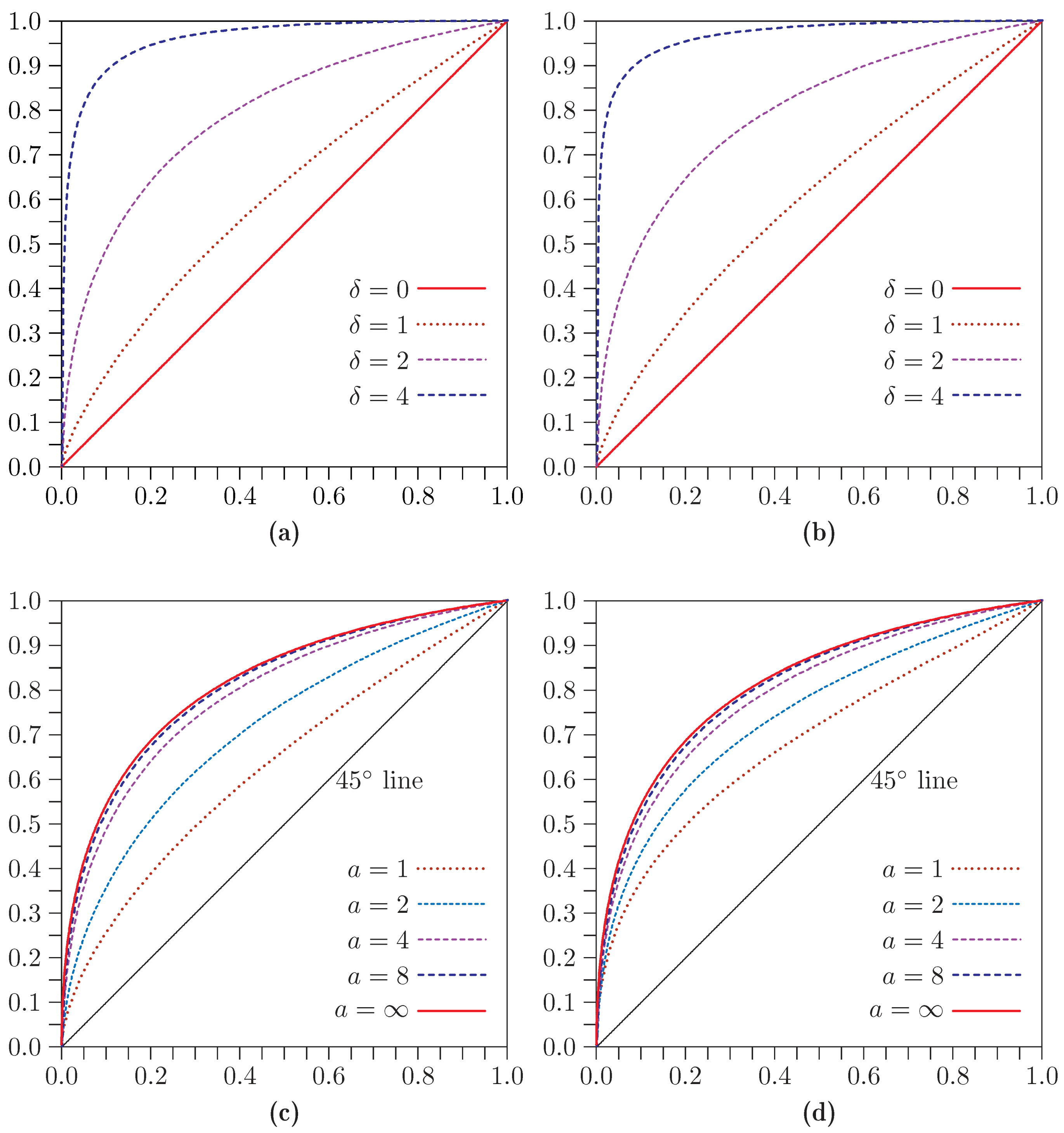
The top two panels of
Figure 13 show size-power curves for
,
, and four values of
δ. Perhaps surprisingly, the curves for LR
in the left-hand panel look remarkably similar to the ones for
in the right-hand panel. The apparently greater power of
, which is evident in the top right panel of
Figure 12, seems to be almost entirely accounted for by its greater tendency to reject under the null.
The bottom two panels of
Figure 13 show size-power curves for
,
, and four values of
a. It is clear that power increases with
a, but at a decreasing rate. As
, the curves converge to the one given by asymptotic theory, where the distribution under the null is central
and the one under the alternative is noncentral
. This curve is graphed in the figure and labelled
.
The asymptotic result that the test statistics follow the
distribution suggests that only the product
influences power, and that, in particular, there should be no power beyond the level of the test when
. In finite samples, things turn out to be more complicated, as can be seen from
Figure 14, which plots power against
θ for
. The top two panels show results for
and
. The
test has substantial power when
and
, which presumably reflects its tendency to overreject severely under the null when the instruments are weak. Those panels also show, once again, that
can reject far more often than LR
when the instruments are weak. This is much less evident in the bottom two panels, which show results for larger values of
a, namely, 6 and 8.
One surprising feature of
Figure 14 is that, in all cases, power initially increases as
θ increases from 0, even though
declines. This is true even for quite large values of
a, such as
, although, of course, it is not true for extremely large values.
Figure 13.
Size-power curves for , , , and . (a) LR: and several values of δ; (b) : and several values of δ; (c) LR: and several values of a; (d) : and several values of a.
Figure 13.
Size-power curves for , , , and . (a) LR: and several values of δ; (b) : and several values of δ; (c) LR: and several values of a; (d) : and several values of a.
Figure 14.
Power as a function of θ for , , and . (a) ; (b) ; (c) ; (d)
Figure 14.
Power as a function of θ for , , and . (a) ; (b) ; (c) ; (d)
9. Relaxing the IID Assumption
The resampling bootstraps that we looked at in
Section 7 do not implicitly make the assumption that the disturbances are normal. They do, however, assume that the disturbances are pairwise IID. If instead the disturbances are heteroskedastic, then the covariance matrix of their bivariate distribution may be different for each observation. In that case, all the test statistics we have studied have distributions that depend on the pattern of heteroskedasticity, and so they are no longer approximately pivotal for the model (1) and (2) under either weak-instrument or strong-instrument asymptotics.
Andrews, Moreira, and Stock [
21] proposes heteroskedasticity-robust versions of test statistics for tests about the value of
β that are robust to weak instruments. Note that, although Andrews, Moreira, and Stock [
6] is based on the 2004 paper and has almost the same title, it does not contain this material. However, this work cannot be applied here, because, as we have seen, the overidentification tests are not robust to weak instruments.
The role of the denominators of the statistics
S,
, and LR
is simply to provide non-robust estimates of the scale of the numerators. In order to make those statistics robust to heteroskedasticity, we have to provide robust measures instead. The numerators of all three statistics can be written as
where the vector
denotes either
, in the case of
S and
, or
, in the case of LR
. Expression (
48) is a quadratic form in the
-vector
. The usual estimate of the covariance matrix of that vector is
, where
. Thus the heteroskedasticity-robust variant of all three test statistics is the quadratic form
There would be no point in using a heteroskedasticity-robust statistic along with a bootstrap DGP that imposed homoskedasticity. The natural way to avoid doing so is to use the wild bootstrap. In Davidson and MacKinnon [
8], the wild bootstrap is shown to have good properties when used with tests about the value of
β. The disturbances of the wild bootstrap DGP are given by
where
is an auxiliary random variable with expectation 0 and variance 1. The easiest choice for the distribution of the
is the Rademacher distribution, which sets
to
or
, each with probability one half. This is also probably the best choice in most cases; see Davidson and Flachaire [
22].
The IID assumption can, of course, be relaxed in other ways. In particular, it would be easy to modify the test statistic (
49) to allow for clustered data by replacing the middle matrix with one that resembles the middle matrix for the usual cluster robust covariance matrix. We could then use a variant of the wild cluster bootstrap of Cameron, Gelbach, and Miller [
23] that allows for simultaneity. The Rademacher random variable associated with each cluster, the analog of
in Equation (
50), would then multiply the residuals for all observations within that cluster for both equations.


