Evaluating Eigenvector Spatial Filter Corrections for Omitted Georeferenced Variables

Abstract

The Ramsey regression equation specification error test (RESET) furnishes a diagnostic for omitted variables in a linear regression model specification (i.e., the null hypothesis is no omitted variables). Integer powers of fitted values from a regression analysis are introduced as additional covariates in a second regression analysis. The former regression model can be considered restricted, whereas the latter model can be considered unrestricted; this first model is nested within this second model. A RESET significance test is conducted with an F-test using the error sums of squares and the degrees of freedom for the two models. For georeferenced data, eigenvectors can be extracted from a modified spatial weights matrix, and included in a linear regression model specification to account for the presence of nonzero spatial autocorrelation. The intuition underlying this methodology is that these synthetic variates function as surrogates for omitted variables. Accordingly, a restricted regression model without eigenvectors should indicate an omitted variables problem, whereas an unrestricted regression model with eigenvectors should result in a failure to reject the RESET null hypothesis. This paper furnishes eleven empirical examples, covering a wide range of spatial attribute data types, that illustrate the effectiveness of eigenvector spatial filtering in addressing the omitted variables problem for georeferenced data as measured by the RESET.

1. Introduction

A practitioner spends considerable time contemplating which covariates to include in a descriptive regression equation, as well as the functional forms they should have. A serious problem in regression analysis is misspecification of a descriptive equation by failing to include all relevant covariates in it: the omitted variables problem. One result of such omissions is omitted-variable bias (OVB), which arises when parameter estimates for the covariates included in a descriptive equation are over- or under-estimated because estimation attempts to compensate for the omitted variables. In part, this outcome arises from multicollinearity; in part, this outcome arises from a biased error variance estimate (i.e., covariates being removed from a specification because they are deemed insignificant when they are significant). A serious linear regression consequence of OVB for ordinary least squares (OLS) estimation is biased and inconsistent parameter estimates. OVB also impacts on non-linear regression.

The Ramsey (1969) [1] regression equation specification error test (RESET) furnishes a tool to at least partially assess OVB. Technically, it is not about omitted variables, but rather it is about functional form (e.g., Wooldridge 2013 ([2], Chapter 9)). It addresses the question asking whether or not non-linear combinations of fitted values help explain a response variable. Its supporting logic contends that non-linear combinations (e.g., exponential powers and cross-products) of covariates that correlate with a response variable signify a mis-specified equation. Consequently, the RESET specifically tests functional form, but often with inferences drawn about omitted variables. Shukur and Mantalos (2004) [3] comment that the RESET has good statistical power with increasing misspecification, and as the RESET proxy variate more closely approximates omitted variables. Of note is that the only way to truly assess OVB is to have the omitted variables to assess, which is not practical.

Studies (e.g., Brasington and Hite 2005 [4], Pace and LeSage 2010 [5]) show that spatial models accommodating spatial dependence are less influenced by OVB, especially when a true data generating process contains a spatial dependence component. Comparisons of model specifications between non-spatial and/or spatial models already appear in the literature. LeSage and Parent (2007) [6] investigate OVB with different model specifications, including ones for non-spatial and spatial regression, using a Bayesian model averaging technique. LeSage and Fischer (2008) [7] and Piribauer and Fischer (2015) [8] extend this approach for model uncertainty in spatial growth modeling. Piribauer (2016) [9] further extends it using stochastic search variable selection priors to improve OVB as well as over-parameterization.

The purpose of this paper is to demonstrate how eigenvector spatial filtering (ESF) impacts OVB as measured by the RESET. As a popular alternative approach for spatial regression model specification (Griffith 2003 [10], Pace, LeSage, and Zhu 2013 [11], Chun and Griffith 2014 [12]), ESF offers the potential to alleviate OVB by including spatial dependence components.

2. The RESET for a Linear Regression Specification

Ramsey (1969) [1] formulated his test for the case of linear regression. His test begins with the conditional expectation

$$\mathrm{E}\left(Y|X\right)=X\mathsf{\beta }$$

(1)

where Y is an n-by-1 vector of response values, hat (the diacritical mark) denotes fitted value, E denotes the calculus of expectation operator, X is an n-by-(p + 1) matrix containing p covariates (p must be at least 1 here), n is the number of observations, and $\mathsf{\beta }$ is a (p + 1)-by-1 vector of regression coefficients. If some n-by-q matrix of covariates Z is incorrectly omitted from this regression equation, in the case where X and Z are non-stochastic, then

$$\mathrm{E}\left(\widehat{\mathsf{\gamma }}\right)={\left(X^{\mathrm{T}}X\right)}^{-1}{X}^{\mathrm{T}}\left(X\mathsf{\beta }+Z\mathsf{\theta }\right)=\mathsf{\beta }+\mathrm{bias}$$

(2)

where superscript T denotes the matrix transpose operation, $\mathsf{\theta }$ denotes regression coefficients for the covariates Z, and $\mathsf{\gamma }$ denotes the full set of regression coefficients. If X^TZ = 0, which is highly unlikely in practice, then no OVB is present, emphasizing the relationship between OVB and multicollinearity.

If the covariate matrix in Equation (2) is expanded to (X Z), then E($\widehat{\mathsf{\gamma }}$) = $\left(\begin{array}{c}\mathsf{\beta }\\ \mathsf{\theta }\end{array}\right)$. Therefore, if this covariate matrix can be augmented with proxy covariates that approximate matrix Z (or at least the part of Z correlated with X), then the OVB decreases, converging on zero as the approximation becomes increasingly better. Thursby and Schmidt (1977) [13] discuss that an approximation being correlated with omitted variables can lead to a powerful test. The RESET uses exponential powers of $X\mathsf{\beta }$ for this approximation. Accordingly, matrix X must contain more than the vector of ones (for the intercept term). The resulting set of equations for testing purposes is given by

$$Y=X\mathsf{\beta }+{\displaystyle \sum }_{\mathrm{k}=1}^{\mathrm{K}}{\mathsf{\phi }}_{\mathrm{k}}{\widehat{Y}}^{\mathrm{k}}+\mathsf{ϵ}$$

(3)

where ${\widehat{Y}}^{\mathrm{k}}={\left(X\widehat{\mathsf{\beta }}\right)}^{\mathrm{k}}$ for integer k ≥ 2, and $\mathsf{ϵ}$ is a n-by-1 vector of random errors for a non-spatial model. The joint null hypothesis for the ${\mathsf{\phi }}_{\mathrm{k}}$ coefficients is that all of them are zero, which is tested using the F-ratio

[(ESS₁ − ESS₂)/(df₂ − df₁)]/[ESS₂/(n-df₂)]

where ESS_j and df_j are, respectively, the error sum of squares and the degrees of freedom for model j (j = 1, 2, …). Rejection of the null hypothesis implies misspecification. When implementing Equation (3), in order to exploit the spatial autocorrelation common to X and Z, as well as the spatial autocorrelation unique to Z, our analyses used exponential powers of fitted values from an eigenvector spatial filter for this approximation: $\widehat{Y}=X\widehat{\mathsf{\beta }}+E_{\mathrm{h}}{\widehat{\mathsf{\beta }}}_{\mathrm{h}}$, where E_h are the eigenvectors discussed in Section 4. That is, an ESF model can be expressed as

$$Y=X\mathsf{\beta }+E_{\mathrm{h}}{\widehat{\mathsf{\beta }}}_{\mathrm{h}}+{\displaystyle \sum }_{\mathrm{k}=1}^{\mathrm{K}}{\mathsf{\phi }}_{\mathrm{k}}{\widehat{Y}}^{\mathrm{k}}+\mathsf{ϵ}$$

(4)

3. The RESET for a Generalized Linear Regression Specification

Sapra (2005) [14] extends Ramsey’s RESET to generalized linear models (GLMs). The logic remains the same here; the response variable no longer is a normal random variable (RV). Rather, it is a Poisson, binomial, or other RV from the exponential family.

The basic equation is similar to (3): assessment is in terms of powers of a linear combination of covariates. For a Poisson RV, the linear combination is the log-mean estimate. For a binomial random variable, the linear combination is the log-odds ratio function. The test statistic is the chi-square, whereas the calculation is −2 times the log-likelihood function differences (subtracting that for the expanded specifications from the original specification). Sapra (2005) [14] comments that this extended version of the RESET appears to have reasonable statistical power for medium to large sample sizes.

4. Eigenvector Spatial Filtering and Omitted Variables

One contention about the presence of non-zero spatial autocorrelation in regression residuals is that it arises because covariates with spatial patterns are missing from a descriptive equation specification (e.g., Temple 1999 [15]). Shifting this spatial autocorrelation from the residuals to the systematic part of the equation (e.g., introducing a spatial autoregressive term) furnishes a surrogate for the missing variable(s), which can be seen by, for example, an increase in the accompanying pseudo-R² value. But auto-models are complicated. ESF offers a simpler approach to handling this omitted variables problem. In other words, because spatial autocorrelation can arise from a missing relevant variable that has an underlying spatial map pattern, a spatial filter constructed with eigenvectors that shows this same underlying spatial autocorrelation pattern can serve as a proxy for missing variables by accounting for spatial autocorrelation.

ESF uses a set of synthetic proxy variables, which are extracted as eigenvectors from an adjusted spatial weights matrix C (defined in Equation (5)) that links geographic objects together in space, and then adds these vectors as control variables to an equation specification. These control variables identify and isolate the stochastic spatial dependencies among a given set of georeferenced observations, resulting in their mimicking independent ones, thus allowing spatial statistical analysis to proceed in standard ways. Spatial autocorrelation in regression residuals often arises because of a missing relevant variable that has an underlying spatial pattern (e.g., McMillan 2003 [16]). Thus, a spatial filter constructed with eigenvectors that exhibit appropriate spatial autocorrelation patterns can serve as a proxy by accounting for spatial autocorrelation.

ESF applies the mathematical decomposition that creates eigenfunctions to the following transformed spatial weights matrix:

$$\left(I-{\mathbf{11}}^{\mathrm{T}}/n\right)C\left(I-{\mathbf{11}}^{\mathrm{T}}/n\right)$$

(5)

where I is an n-by-n identity matrix, and 1 is an n-by-1 vector of ones. This decomposition generates n eigenvectors and their associated n eigenvalues. In descending order, the n eigenvalues can be denoted as λ = (λ₁, λ₂, λ₃, …, λ_n), ranging between the largest eigenvalue that is positive, λ₁, and the smallest eigenvalue that is negative, λ_n. The corresponding n eigenvectors can be denoted as E = (E₁, E₂, E₃, …, E_n), where each eigenvector, E_j, is an n-by-1 vector.

These eigenfunctions have a number of important properties. First, the eigenvectors are mutually orthogonal and uncorrelated (Griffith 2000) [17]: the symmetry of matrix C ensures orthogonality, and the projection matrix $\left(I-{\mathbf{11}}^{\mathrm{T}}/n\right)$ ensures that eigenvectors have zero means, guaranteeing uncorrelatedness. That is, EE^T = I and E^T1 = 0, and the correlation between any pair of eigenvectors, say E_i and E_j, is zero when i ≠ j. Second, the eigenvectors portray distinct, selected map patterns. Tiefelsdorf and Boots (1995) [18] establish that each eigenvector portrays a different map pattern exhibiting a specified level of spatial autocorrelation when it is mapped onto the n areal units associated with the corresponding spatial weights matrix C. They also establish that the Moran coefficient (MC) value for a mapped eigenvector is equal to a function of its corresponding eigenvalue (i.e., MC_j = $\frac{\mathrm{n}}{1^{\mathrm{T}}C1}\cdot {\mathsf{\lambda }}_j$, for E_j). Third, given a spatial weights matrix C, the feasible range of MC values is determined by the largest and smallest eigenvalues; i.e., by λ₁ and λ_n (de Jong et al. 1984) [19]. Based upon these properties, the eigenvectors can be interpreted as follows (Griffith 2003) [10]:

The first eigenvector, E₁, is the set of real numbers that has the largest MC value achievable by any set of real numbers for the spatial arrangement defined by the spatial weight matrix C; the second eigenvector, E_2, is the set of real numbers that has the largest achievable MC value by any set that is uncorrelated with E₁; the third eigenvector, E₃, is the set of real numbers that has the largest achievable MC value by any set that is uncorrelated with both E₁ and E₂; the fourth eigenvector is the fourth such set of values; and so on through E_n, the set of real numbers that has the largest negative MC value achievable by any set that is uncorrelated with the preceding (n − 1) eigenvectors.

As such, these eigenvectors furnish distinct map pattern descriptions of latent spatial autocorrelation in spatial variables, because they are mutually both orthogonal and uncorrelated.

ESF furnishes a promising alternative approach to the popular spatial auto-model for describing a spatial process. Pace, LeSage, and Zhu (2013) [11] comment that ESF is an effective method to alleviate OVB. With a simulation experiment that examines ESF estimates for two different types of data generating processes (i.e., spatial autoregressive and spatial error processes), they find that ESF reduces bias in parameter estimates. One appealing feature of ESF is that it utilizes a relevant subset of eigenvectors extracted from a spatial weights matrix, whereas a spatial autoregressive model utilizes the full set of these eigenvectors, both ones that correlate and ones that do not correlate (and hence introduce noise) with the response variable in question. Another appealing feature of ESF is that determining its associated degrees of freedom is more straightforward; a spatial autoregressive model has a complicated degrees of freedom structure because of its multiplicative form. The number of degrees of freedom for the spatial autocorrelation parameter can differ from 1 (Janson, Fithian, and Hasatie 2015) [20].

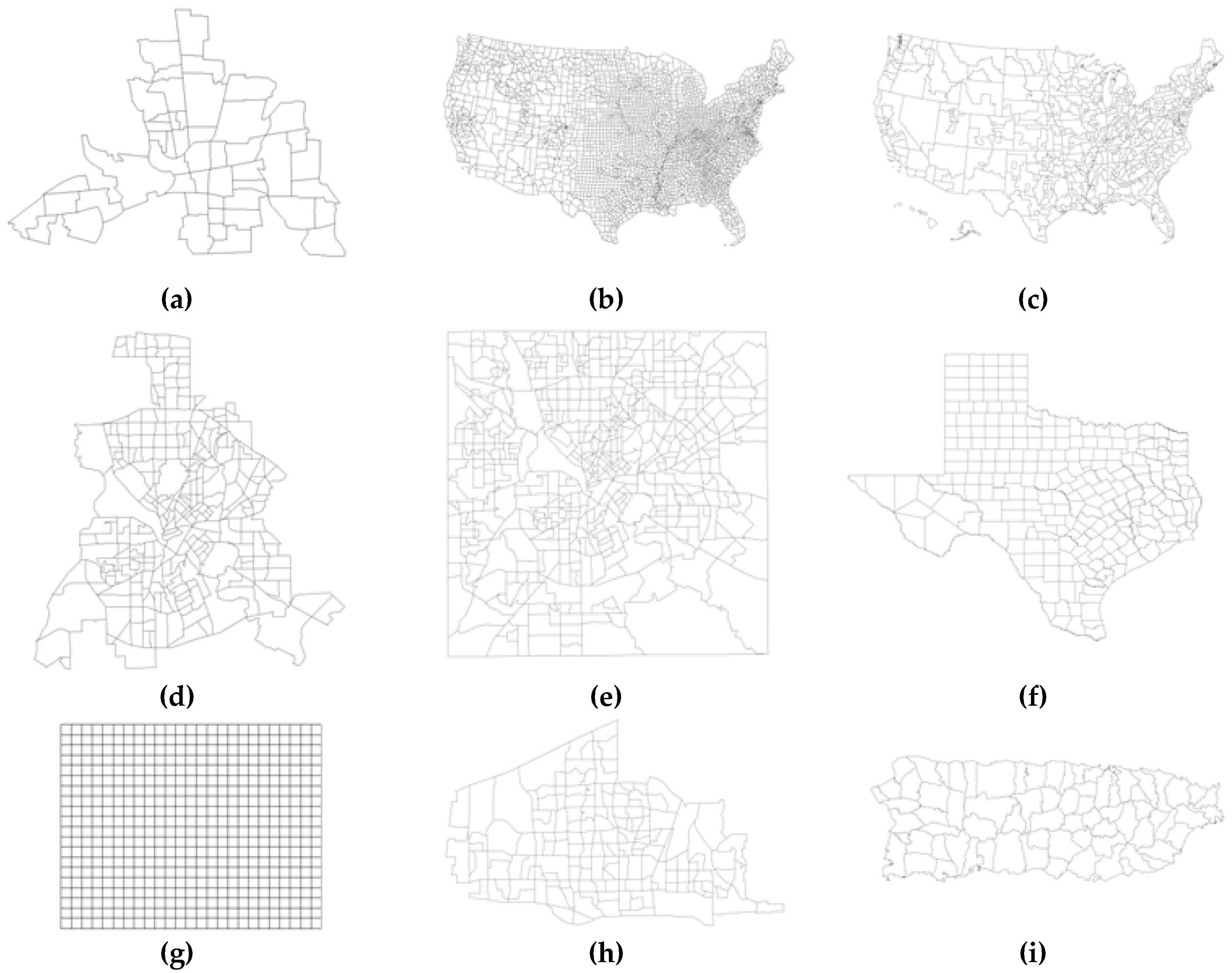
5. Specimen Empirical Datasets

Illustrative analyses have been completed with eleven empirical datasets1 that span a range of sample sizes (49 to 3109): Dallas, TX City and County census tracts; United States (US) state economic areas (SEAs); US as well as Texas counties; Anselin’s Columbus neighborhoods; Plano, TX block groups; Mercer-Hall agricultural field plots; and, Puerto Rico municipalities. Figure 1 portrays the various surface partitionings associated with these datasets.

For the linear model specification coupled with a normal probability model, several of the response variables need to be subjected to a Box-Cox power transformation. Puerto Rican irrigated farm counts have been analyzed with both a normal approximation (for their density version) and a binomial generalized linear model specification (for their percentage version). Finally, Texas cancer counts have been analyzed with a Poisson generalized linear model specification.

Crime data are: 1980 for Columbus, OH; 2008 for Plano, TX (vehicle burglary); and, 2010 for the City of Dallas. Population density data are: 2010 for Dallas, TX, and for the US. Mercer-Hall crop data are 1910 wheat yields. Puerto Rico irrigated farms data are: 2007 for density; and, 2002 for percentages. US SEA white male prostate cancer rates are age-adjusted for 1970–1994. Finally, Texas county cancer counts are for 2003, whereas Texas county mortgage data are for 2000.

These datasets not only furnish a range of sizes, but Figure 1 reveals that they also furnish a wide range of qualitatively different surface partitionings. In addition, they furnish a range of covariate set sizes, as well as a range of response variable types that includes examples of each of the three most commonly encountered varieties of georeferenced RVs (e.g., normal, binomial, and Poisson).

6. RESET Results for the Specimen Empirical Datasets

The RESET for an ESF model was conducted with the selected eigenvectors as additional independent variables. That is, the F-test was calculated with the sums of squared errors for the ESF model and its counterpart with additional fitted value terms.2 Inclusion of a constructed eigenvector spatial filter improves the RESET analysis in all eleven cases (

Table 1. Ramsey regression equation specification error test (RESET) results for the linear model empirical examples.

Data	n	Y	X	RESET Non-Spatial Model				RESET Spatial Model (ESF)
				R2	RESET	DF1, DF2	p-Value	R2	RESET	DF1, DF2	p-Value
Columbus	49	Crime rates	Housing value, household income	0.5524	1.6122	5, 41	0.1784	0.7419	1.4361	5, 38	0.2337
Puerto Rico	73	Irrigated farm density	Mean rainfall	0.1383	1.8075	5, 66	0.1235	0.4686	1.4361	5, 60	0.2245
Plano Census Block groups	159	Box-Cox 1 transformed Vehicle Burglary rates	Rates of population aged between 18 and 24, Distance to highway	0.1428	4.7558	5, 151	0.0005	0.4169	1.5777	5, 142	0.1701
Texas Counties	254	Median Monthly Mortgage	Log of Population Density, Log of Household Median Income, % of housing units built since 1980	0.7740	10.5403	5, 245	3.5 × 10−9	0.8597	3.6297	5, 228	0.0035
City of Dallas Census Tracts	264	Log of violation crime rates in 2000	Rates of population aged between 13 and 17, Black population rates, Poverty rate	0.5336	20.6077	4, 256	9.8 × 10−15	0.7374	1.9273	4, 245	0.1065
Mercer Hall	500	Wheat yield	Straw yield	0.5326	3.9194	3, 496	0.0088	0.7376	0.991	4, 455	0.4121
US SEA	508	White male Prostate cancer rates	White male Bladder cancer rate, Mean indoor radon concentration	0.1392	4.0884	5, 500	0.0012	0.4857	0.3308	5, 470	0.8943
Dallas County Census tracts	529	Box-Cox 2 transformed Pop. Density	Y coordinates, # of families, Log of distance to CBD	0.1671	11.9806	3, 522	1.3 × 10−7	0.5949	1.2653	3, 472	0.2857
US Counties	3109	Log of population density	Log of # of families, Old population rates (60+)	0.7394	13.8545	5, 3101	2.1 × 10−13	0.8952	4.4681	5, 2894	0.0005

¹ The Box-Cox transformation was performed with $(y^{\mathsf{\lambda }}-1)/\mathsf{\lambda }$ where $\widehat{\mathsf{\lambda }}=-0.1113$. ² The Box-Cox transformation was performed with $\widehat{\mathsf{\lambda }}=0.3408$.

and

Table 2. RESET results for the generalized linear model (GLM) empirical examples.

Term	Before ESF		After ESF
	${\mathit{\chi }}^{\mathbf{2}}$	p-Values	${\mathit{\chi }}^{\mathbf{2}}$	p-Values
Puerto Rico (Binomial): Irrigate farms (y) with log of mean rainfall (x)
${\widehat{\text{Y}}}^2$	0.4510	0.5018	0.0003	0.9853
${\widehat{\text{Y}}}^3$	100.7835	<2.2 × 10−16	16.2781	0.0003
Pseudo-R2	0.4528		0.4829
Texas counties (Poisson): Cancer counts (y) with three covariates 1
${\widehat{\text{Y}}}^2$	127.3967	<2.2 × 10−16	3.5006	0.0614
${\widehat{\text{Y}}}^3$	147.8025	<2.2 × 10−16	18.2274	0.0001
Pseudo-R2	0.1315		0.3722

¹ The covariates are log of household median income, log of white population rates, and log of single marital status rates.

). This improvement is of three types: when the diagnostic fails to indicate omitted variables; when the diagnostic indicates omitted variables before, but not after, adding an eigenvector spatial filter; and, when the diagnostic still indicates omitted variables after inclusion of an eigenvector spatial filter.

In all cases, inclusion of an eigenvector spatial filter increases the (pseudo-)R², sometimes more than tripling it. Both Columbus, OH crime rates, and Puerto Rico density of irrigated farms include covariates that do not yield a RESET diagnostic suggesting omitted variables; nevertheless, inclusion of an eigenvector spatial filter increases the null hypothesis (no omitted variables) RESET probability.

Plano vehicle burglary rates, City of Dallas crime rates, Mercer-Hall wheat yield, US SEA prostate cancer rates, and Dallas County population density have an initial RESET diagnostic suggesting omitted variables, and a RESET diagnostic with a probability of at least 0.1 after inclusion of an eigenvector spatial filter. The implication here is that an eigenvector spatial filter substitutes well for omitted variables.

Texas median monthly mortgages, US population density, and GLM results for both percentage of Puerto Rican irrigated farms and Texas cancer counts have RESET diagnostics that indicate the presence of omitted variables both with and without inclusion of an ESF. Inclusion of an ESF increases the RESET probabilities, but not enough for them to be non-significant. These may be cases in which a spatially unstructured term also is needed to compensate for omitted variables.

For comparison purposes, a RESET was conducted for spatial lag and spatial error model specifications using the Columbus dataset. Here, because of their non-linear forms, the RESET employs the chi-square test for the likelihood ratio difference between a restricted model and its unrestricted counterpart (Vaona 2009) [21]. That is, integer powers of (z-score versions of) fitted values from a spatial regression model are introduced as explanatory variables. Here the resulting RESET p-values are 0.3663 and 0.1852, respectively, whereas the resulting pseudo-R² values are 0.6523 and 0.6584, respectively. These findings suggest that spatial autoregressive models also correct for OVB, offering spatial analysts two ways of exploiting spatial autocorrelation to compensate for omitted variables.

Cross-Validation RESET Results for the Specimen Empirical Datasets

Each of the specimen datasets was subjected to a cross-validation evaluation to examine the sensitivity of the RESET to individual observations, with each observation in a dataset being left out, in turn, and then predicted.

Table 3. RESET cross-validation results for the specimen linear models.

Data	n	Maintained p ≤ 0.1	Improved from p ≤ 0.1 to p > 0.1	Declined from p > 0.1 to p ≤ 0.1	Maintained p > 0.1
Columbus	49	0	2	2	45
Puerto Rico	73	0	6	2	65
Plano Census Block Groups	159	92 1	67	0	0
Texas Counties	254	254 2	0	0	0
City of Dallas Census Tracts	264	261 3	3	0	0
Mercer Hall	500	4	495	0	1
US SEA	508	0	507	0	1
Dallas County Census Tracts	529	0	528	1	0
US Counties	3109	3019 4	0	0	0

¹ p-values for 35 (out of 92) cases increased from less than 0.0001 to greater than 0.05. ² p-values for 252 (out of 254) cases increased from less than 10⁻⁷ to greater than 0.001. ³ p-values for 256 (out of 261) cases increased from less than 10⁻⁹ to greater than 0.001. ⁴ p-values of 3104 (out of 3109) cases increased from less than 10⁻¹⁰ to greater than 0.0001.

summarizes results for the linear model examples, and

Table 4. RESET cross-validation results for the specimen generalized linear models.

Term	n	Maintained p ≤ 0.1	Improved from p ≤ 0.1 to p > 0.1	Declined from p > 0.1 to p ≤ 0.1	Maintained p > 0.1
Puerto Rico (Binomial): Irrigate farms (y) with log of mean rainfall (x)
${\widehat{\text{Y}}}^2$	73	0	1	70	2
${\widehat{\text{Y}}}^3$	73	72 1	1	0	0
Texas counties (Poisson): Cancer counts (y) with three covariates 1
${\widehat{\text{Y}}}^2$	254	246	8	0	0
${\widehat{\text{Y}}}^3$	254	253 2	1	0	0

¹ The p-values of 70 cases (out of 72) increased from one less than 1.0 × 10⁻¹⁶ to one greater than 1.0 × 10⁻⁵, and for 12 cases of them, increased to one greater than 0.0001. ² The p-values of 252 cases (out of 253) increased from one less than 1.0 × 10⁻¹⁶ to one greater than 1.0 × 10⁻⁵, and for 190 cases of them, increased to one greater than 0.0001.

summarizes results for the generalized linear model examples. These results are encouraging, given the number of improvements, but indicate the need for further refinement work in this area. The goal would be for almost all, if not all, of the cases to improve, achieving a RESET probability exceeding 0.1.

7. Correction for Omitted Variable Bias: Selected Simulation Experiments

OVB results in an estimated regression coefficient differing substantially from its population parameter, often in an attempt by included covariates to compensate for omitted variables. This substantial difference can render an incorrect null hypothesis test result concerning included variables. Empirical evidence presented here suggests that an eigenvector spatial filter helps remediate this situation.

The first simulation experiment summarized here is based upon the Puerto Rico (n = 73) agricultural dataset. The response variable is the sum of the density of farms using irrigation (X₁) and Box-Tidwell transformed mean rainfall (X₂), plus an independent and identically distributed (iid) random error term that is N(0, 0.1²). The correlation between the two covariates is 0.43, indicating modest collinearity. The response variable (containing 73 values) was simulated 10,000 times, followed by estimation of its linear regression equation as well as each of the two individual bivariate regression equations, resulting in

$$\begin{array}{l}\overline{\widehat{Y}}={\overline{\widehat{\mathsf{\beta }}}}_{0}1+1.00046X_1+0.99996X_2\\ \overline{\widehat{Y}}={\overline{\widehat{\mathsf{\beta }}}}_{0}1+1.42810X_1\\ \overline{\widehat{Y}}={\overline{\widehat{\mathsf{\beta }}}}_{0}1+1.42419X_2\\ {\widehat{Y}}_j={\widehat{\mathsf{\beta }}}_{0\text{j}}1+E_{kj}{\mathsf{\beta }}_{\text{kj}},\mathrm{j}=1,2,...,\mathrm{10,000}\end{array}$$

The intercept term estimate is not reported here because it is not of interest. The average regression coefficient estimates of 1.00046 and 0.99996 are not different from 1 (standard errors of roughly 0.049), their population parameter counterparts (i.e., the true model). The bivariate regression coefficient estimates indicate that the OVB is sizeable, exceeding 42%, and significant (standard errors of 0.044). Powers of the eigenvector spatial filter fitted values (${\widehat{Y}}_j$) furnish the RESET terms for simulation replicate j.

Table 5. Selection frequency of RESET terms for the Puerto Rico simulation experiment.

Variable	None	${\widehat{Y}}^{\mathbf{2}}$	${\widehat{Y}}^{\mathbf{3}}$	${\widehat{Y}}^{\mathbf{4}}$	${\widehat{Y}}^{\mathbf{2}}$&${\widehat{Y}}^{\mathbf{3}}$	${\widehat{Y}}^{\mathbf{2}}$&${\widehat{Y}}^{\mathbf{4}}$	${\widehat{Y}}^{\mathbf{3}}$&${\widehat{Y}}^{\mathbf{4}}$	${\widehat{Y}}^{\mathbf{2}}$&${\widehat{Y}}^{\mathbf{3}}$&${\widehat{Y}}^{\mathbf{4}}$
X1	0	843	4607	4282	0	4	210	54
X2	0	1673	4660	3666	0	1	0	0

summarizes outcomes of this simulation experiment, which involved stepwise selection of the RESET terms (which are constructed from eigenvector spatial filters). The average bivariate regression coefficient estimates corrected by the RESET are 0.95574 and 0.94882, both of which are markedly less than their OVB counterparts, although they are modestly deflated. Their respective standard errors are 0.062 and 0.067, which, unlike the original OVB estimates, mean they are not significantly different from 1.

The second simulation experiment summarized here is based upon the Texas (n = 254) cancer dataset. The response variable is the exponentiated weighted sum of the logarithms of median household income (X₁), percentage of white population (X₂), and percentage of single (i.e., unmarried) people (X₃), plus log-total population as an offset variable. The weights are the Poisson regression coefficients from a GLM. Because the expectation equation is a description of cancer counts that are overdispersed, it was used as the mean of a gamma RV, whose sampled values were treated as means of Poisson RVs.3 The response variable (containing 254 values) was simulated 10,000 times, followed by estimation of its Poisson GLM equation as well as each of the three individual bivariate and individual trivariate binomial regression equations, resulting in

$$\begin{array}{l}\overline{\widehat{Y}}=\exp \left[{\overline{\widehat{\mathsf{\beta }}}}_{0}1-0.30X_1+0.20X_2-0.80X_3+LN(population)\right]\\ \overline{\widehat{Y}}=\exp \left[{\overline{\widehat{\mathsf{\beta }}}}_{0}1-0.46X_1+LN(population)\right]\\ \overline{\widehat{Y}}=\exp \left[{\overline{\widehat{\mathsf{\beta }}}}_{0}1+1.05X_2+LN(population)\right]\\ \overline{\widehat{Y}}=\exp \left[{\overline{\widehat{\mathsf{\beta }}}}_{0}1-0.97X_3+LN(population)\right]\\ \overline{\widehat{Y}}=\exp \left[{\overline{\widehat{\mathsf{\beta }}}}_{0}1-0.32X_1+0.95X_2+LN(population)\right]\\ \overline{\widehat{Y}}=\exp \left[{\overline{\widehat{\mathsf{\beta }}}}_{0}1-0.31X_1-0.90X_3+LN(population)\right]\\ \overline{\widehat{Y}}=\exp \left[{\overline{\widehat{\mathsf{\beta }}}}_{0}1+0.29X_2-0.82X_3+LN(population)\right]\\ {\widehat{Y}}_j=\exp \left({\widehat{\mathsf{\beta }}}_{0\text{j}}1+E_{kj}{\beta }_{\text{kj}}+LN(population\right),\text{j}=1,2,...,\mathrm{10,000}\end{array}$$

Again, the intercept term estimate is not reported here because it is not of interest; however, in some empirical cases, it is of interest, another reason to use the z-score versions of fitted values.

Table 6. Selection frequency of RESET terms for the Texas data simulation experiment.

Variable	None	${\widehat{Y}}^{\mathbf{2}}$	${\widehat{Y}}^{\mathbf{3}}$	${\widehat{Y}}^{\mathbf{4}}$	${\widehat{Y}}^{\mathbf{2}}$&${\widehat{Y}}^{\mathbf{3}}$	${\widehat{Y}}^{\mathbf{2}}$&${\widehat{Y}}^{\mathbf{4}}$	${\widehat{Y}}^{\mathbf{3}}$&${\widehat{Y}}^{\mathbf{4}}$	${\widehat{Y}}^{\mathbf{2}}$&${\widehat{Y}}^{\mathbf{3}}$&${\widehat{Y}}^{\mathbf{4}}$
X1	27	594	566	923	902	553	20	6415
X2	84	677	609	1258	271	364	72	6665
X3	1336	773	251	636	688	500	40	5776
X1 & X2	625	770	499	1025	332	406	60	6283
X1 & X3	1320	809	249	635	533	515	85	5854
X2 & X3	1718	825	287	702	578	517	43	5330

summarizes outcomes of this simulation experiment, which involved stepwise selection of the RESET terms (which, as before, are constructed from eigenvector spatial filters).

The average regression coefficient estimates of −0.30213, 0.21343, and −0.80155 respectively do not differ from −0.3, 0.2, and −0.8 (standard errors of roughly 0.2), their population parameter counterparts. The bivariate and trivariate Poisson regression coefficient estimates indicate that the OVB is sizeable, many being at least 20%, and statistically significant. For the bivariate regressions, the eigenvector spatial filter reduces the OVB as reported in

Table 7. Parameter estimates with OVB and ESF RESET adjustments.

Number of Omitted Variables	Estimate Type	X1	X2	X3
two	Parameter	−0.30	0.20	−0.80
	OVB	−0.46	1.05	−0.97
	ESF RESET adjusted	−0.23	0.90	−0.87
one	OVB	−0.32	0.95
	ESF RESET adjusted	−0.25	0.92
	OVB	−0.31		−0.90
	ESF RESET adjusted	−0.34		−0.97
	OVB		0.29	−0.82
	ESF RESET adjusted		0.39	−0.76

.

For the bivariate cases, the estimates with the ESF RESET adjustment are closer to their true values. Specifically, the estimates for X₁ and X₃ are close to their true values, whereas the adjustment for X₂ is less effective. These results indicate that the ESF adjustment is reasonable in a bivariate regression case, but not so in a trivariate regression case. The correlation structure may play a role here: ${\mathrm{r}}_{{\mathrm{X}}_1{\mathrm{X}}_2}$ = 0.11, ${\mathrm{r}}_{{\mathrm{X}}_1{\mathrm{X}}_3}$ = −0.10, and ${\mathrm{r}}_{{\mathrm{X}}_2{\mathrm{X}}_3}$ = −0.53.

These two empirically based simulation experiments furnish a proof of concept, and indicate that ESFs offer promise for effectively dealing with the OVB problem. Clearly, future research should be devoted to this theme.

8. Implications and Conclusions

Properly testing for OVB requires knowing the omitted variables, which does not help in practice. This situation also can be assessed if instrumental variables are available to use. At least in some cases, an eigenvector spatial filter can be treated like an instrument (see Le Gallo and Paez 2013 [22]). Ramsey’s RESET furnishes a special case test where the omitted variables are nonlinear functions of the included covariates. This paper summarizes findings based upon a set of empirical examples and a pair of conditional simulations suggesting that an ESF often can serve as a surrogate for omitted variables. Inclusion of an eigenvector spatial filter tends to increase the (pseudo-)R² and the RESET null hypothesis probability. Combining an eigenvector spatial filter with a spatially unstructured term to correct for OVB merits subsequent research, too.