
Forecasting US Inflation in Real Time

Board of Governors of the Federal Reserve System, 20th and Constitution Ave NW, Washington, DC 20551, USA
*
Author to whom correspondence should be addressed.
Econometrics 2021, 9(4), 36; https://doi.org/10.3390/econometrics9040036
Submission received: 4 July 2019
/
Revised: 15 September 2021
/
Accepted: 16 September 2021
/
Published: 9 October 2021
(This article belongs to the Special Issue Celebrated Econometricians: David Hendry)
Abstract
:We analyze real-time forecasts of US inflation over 1999Q3–2019Q4 and subsamples, investigating whether and how forecast accuracy and robustness can be improved with additional information such as expert judgment, additional macroeconomic variables, and forecast combination. The forecasts include those from the Federal Reserve Board’s Tealbook, the Survey of Professional Forecasters, dynamic models, and combinations thereof. While simple models remain hard to beat, additional information does improve forecasts, especially after 2009. Notably, forecast combination improves forecast accuracy over simpler models and robustifies against bad forecasts; aggregating forecasts of inflation’s components can improve performance compared to forecasting the aggregate directly; and judgmental forecasts, which may incorporate larger and more timely datasets in conjunction with model-based forecasts, improve forecasts at short horizons.
1. Introduction
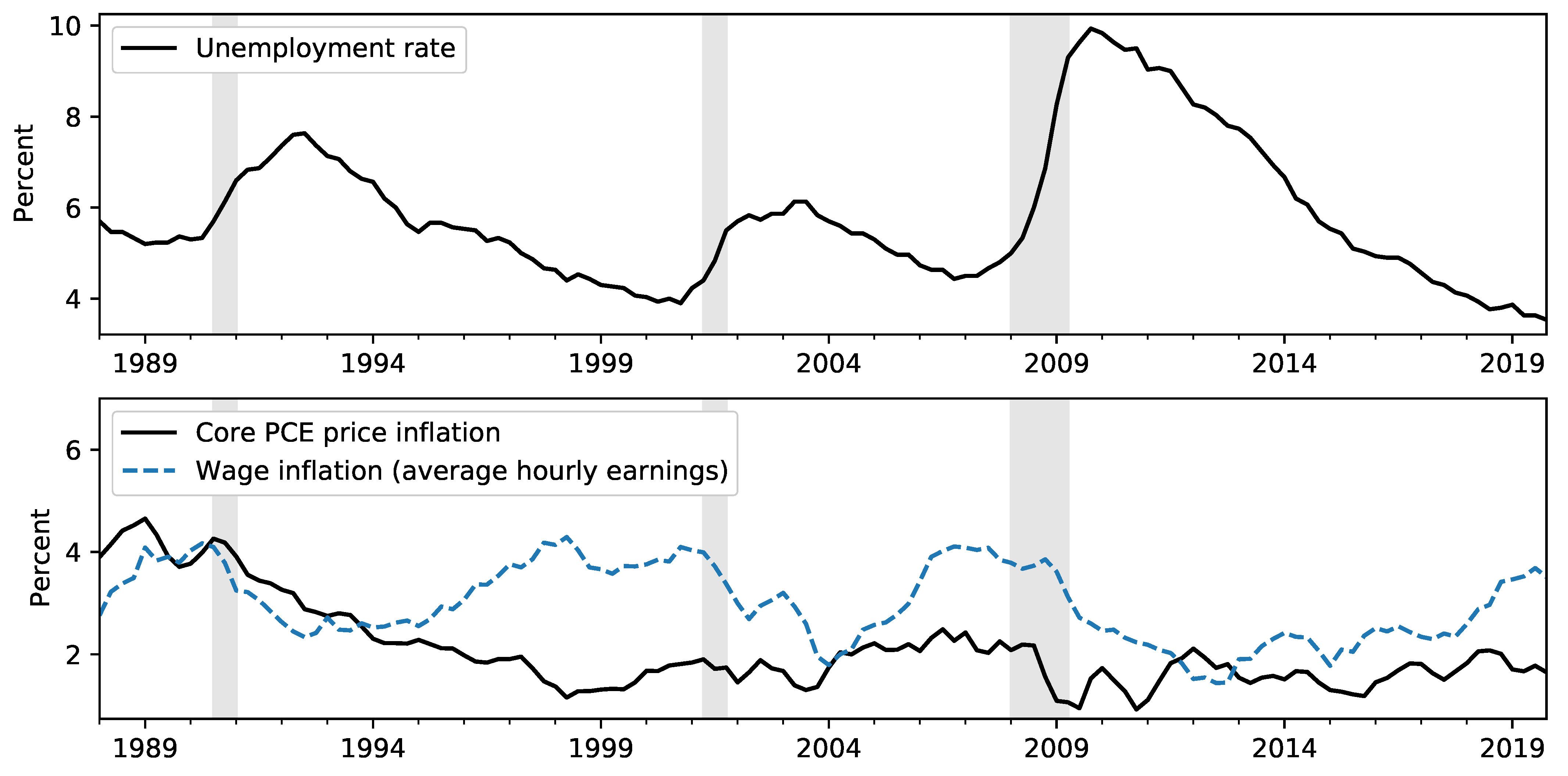
After a slower-than-usual recovery from the Great Recession, the unemployment rate fell to 3.5% in December 2019, its lowest reading since December 1969. At the same time, wage growth, while firming, remained only moderate, and consumer price inflation only briefly reached the 2% target of the Federal Open Market Committee (FOMC). These restrained price movements in the face of dramatic swings in labor market data, illustrated in Figure 1, have been historically puzzling. The current debate about possible inflationary pressures developing highlights the increased uncertainty about the future behavior of inflation and the importance of taking into account a broad information set. Our interest, therefore, is to consider what information, if any, may be used to guide inflation forecasts going forward.
One popular framework for analyzing and forecasting inflation is based on the Phillips curve, the predicted negative relationship between economic slack and inflation. In addition to the extensive literature exploring the empirical and theoretical properties of these models—including the discussion of the recent flattening of the Phillips Curve—former Federal Reserve Board Chair Janet Yellen and current Chair Jerome Powell have in recent speeches referenced an expectations-augmented econometric Phillips curve specification as a framework for modeling and forecasting consumer price inflation.1 At the same time, however, recent literature on inflation forecasting has mostly emphasized simpler, often univariate, models.
In this paper, we investigate if and how additional information—additional macroeconomic variables, expert judgment, or forecast combination—can improve forecast accuracy over simple models. Our key finding is that while simple models remain generally hard to beat, careful introduction of additional information can improve forecasts, particularly in the post-crisis period starting in 2009. Notably, we find aggregating forecasts of inflation components, forecast combination, and using large information sets informing expert judgment to improve forecast accuracy at short horizons.
Our approach is informed by three recent strands of the literature on inflation forecasting. First, Atkeson and Ohanian (2001) and Stock and Watson (2007) show that while inflation has become easier to forecast overall in recent decades—in the sense of lower out-of-sample mean square errors across a variety of univariate and multivariate models mainly due to the overall lower variability of inflation—it has at the same time become more difficult to effectively incorporate information other than inflation itself in producing forecasts that improve over simple benchmark models. In particular, they note that the usefulness of Phillips curve models, in which slack can be used to predict future inflation, appears to have declined.
A second strand of the literature shows that survey forecasts have predictive power for inflation, both when included as an expectations term in Phillips curve models and when considered as direct forecasts. Faust and Wright (2013) distill from previous results and their own real-time forecasting exercise the following lessons: (1) Judgmental forecasts do best; (2) Good forecasts must account for a slowly varying local mean; (3) Good forecasts begin with high quality nowcasts; (4) One of the best forecasting techniques is to simply produce a smooth path between the best available nowcast (as the forecast for the first horizon) and the best available local mean (as the forecast for the last horizon).
We view these results as promising since although all of these papers emphasize the superiority of simple models, each actually incorporates more information in its forecasts than the last. Atkeson and Ohanian (2001) forecast inflation using only its own last four lags, while the unobserved components model with stochastic volatility model introduced by Stock and Watson (2007) allows for time-varying parameters in order to employ the entire history of inflation. In the language of Faust and Wright (2013), each of these papers presented methods for estimating a “local mean” of inflation. Faust and Wright (2013) then extend the local mean to make use of variables other than inflation itself, including judgmental nowcasts and long-term forecasts from surveys that potentially incorporate a large—although poorly defined—additional dataset.
A third strand of the literature explores whether forecast combination can improve inflation forecasts. Forecast combination of different forecasts of the same variable have been shown to improve over the best single forecast in certain situations (see Hendry and Clements (2004)). Furthermore, combining forecasts from disaggregate component models to forecast an aggregate has been found to improve over forecasts from an aggregate model under certain conditions (see, e.g., Lütkepohl (1984), Granger (1987), Hubrich (2005), and Hendry and Hubrich (2011)).
In this paper, we build on these literatures, exploring if and how additional information should inform inflation forecasts. First, we consider incorporating additional information in the form of multivariate inflation forecasting models. We begin by adding specific macroeconomic variables explicitly to econometric models, focusing on resource utilization and inflation expectations as incorporated in an empirical Phillips curve. The economic information contained in these variables is well-defined and can be matched up to theoretical Phillips curve models. We next consider incorporating information from judgmental sources, in particular the Survey of Professional Forecasters (SPF) forecast and the Federal Reserve Board staff forecast presented in the Tealbook (prior to 2010 referred to as Greenbook). The economic information contained in these forecasts is less-well-defined, since it captures both subjective judgment and an unknown range of models and data from a potentially large number of unknown sources.
Second, we investigate incorporating additional information in the form of multiple econometric models, considering both the combination of forecasts from multiple models of overall price inflation and the construction of overall price inflation forecasts by aggregating forecasts of price subcomponents. Specifically, we investigate whether a Phillips Curve specification for overall price inflation improves over forecasting core, energy, and food price inflation separately and then aggregating those forecasts. We also compare this with forecast combination of different models for overall price inflation using different weighting schemes.
Previous literature has mainly focused on aggregation of forecasts from the same model or model class (see, for example, Hubrich (2005), Hendry and Hubrich (2011), and Stock and Watson (2016)). In contrast, we investigate whether forecast performance for US price inflation can be improved by aggregating forecasts with different specifications for each underlying inflation component, allowing us to capture particular time series characteristics of each series. In addition, we investigate whether combining different forecasts of total US price inflation improves forecast performance over the single best forecast. This is particularly relevant in times of economic uncertainty, since forecast combination can potentially be a tool to improve forecast performance in the presence of large changes such as the global financial crisis. Hubrich and Skudelny (2017) find that for Euro area inflation, forecast combination helps to robustify the forecast, since forecast combination for euro area inflation helps improving over the worst forecasts.
To address these questions, we perform a real-time forecasting exercise, focusing on price inflation as measured by the personal consumption expenditures (PCE) chain-type price index employed by the Federal Reserve to evaluate the inflation objective. We extend the real-time forecast evaluation by Faust and Wright (2013) in a number of respects: we explicitly compare different forecast combination and aggregation strategies and include in this analysis SPF and Tealbook forecasts. We also include more recent sample periods and we focus on PCE price inflation (as opposed to other inflation measures such as those based on the GDP deflator or the consumer price index) motivated by its importance for monetary policy in the US. We explore which additional pieces of information were most useful before, during, and after the global financial crisis, and so shed light on which methods are most promising now for constructing and robustifying inflation forecasts. This is particularly relevant in light of the surprising behavior of inflation during the recent expansion and the additional uncertainty that has been introduced by the current, pandemic-induced, economic crisis.
2. Data
Our forecasting exercise focuses on U.S. inflation, measured by the quarter-over-quarter percent change in the personal consumption expenditures (PCE) chain-type price index produced by the Bureau of Economic Analysis (BEA). PCE prices are particularly significant from the perspective of monetary policy, because the longer-run inflation objective of the Federal Open Markets Committee, first adopted in January 2012 and later revised in August 2020, is stated in terms of PCE inflation.2 Nonetheless, other measures of inflation remain important, both as economic indicators and for our exercise here. In Figure 2, we show the evolution of several of these measures.
The primary alternative measure of U.S. consumer price inflation is based on the Consumer Price Index (CPI) published by the Bureau of Labor Statistics (BLS). While this measure differs from the PCE price index in several important ways, it has historically been an important measure for monetary policymakers.3,4 Moreover, while attention has recently shifted to the PCE price index, its construction by the BEA largely relies on source data from disaggregate CPI series collected by the BLS. This fact has implications for our forecasting exercise, because it implies that monthly CPI releases provide information about quarterly PCE price inflation that can be exploited in forecasting.5,6
While the overall PCE price index provides the broadest measure of consumer prices, there is also considerable interest in core inflation measures, which exclude the volatile food and energy subcategories.7 One commonly cited benefit of core measures of inflation is that, since they exclude volatile components, they are better predictors of future inflation. In our exercise, we include a model that aims to take advantage of this by first separately producing forecasts for core, food, and energy prices, and then aggregating to produce a forecast of overall PCE price inflation.
While several of our forecasting models are designed to predict future inflation using only consumer price data, many of the forecasts that we consider make use of other macroeconomic variables, including data on oil prices, prices of imported goods, inflation expectations, and real economic activity. These variables are described in more detail below, when we introduce our forecasting models. We also consider real-time judgmental inflation forecasts produced by the Survey of Professional Forecasters and the Federal Reserve Board, and this introduces several issues related to forecast timing and data availability, which we discuss now.
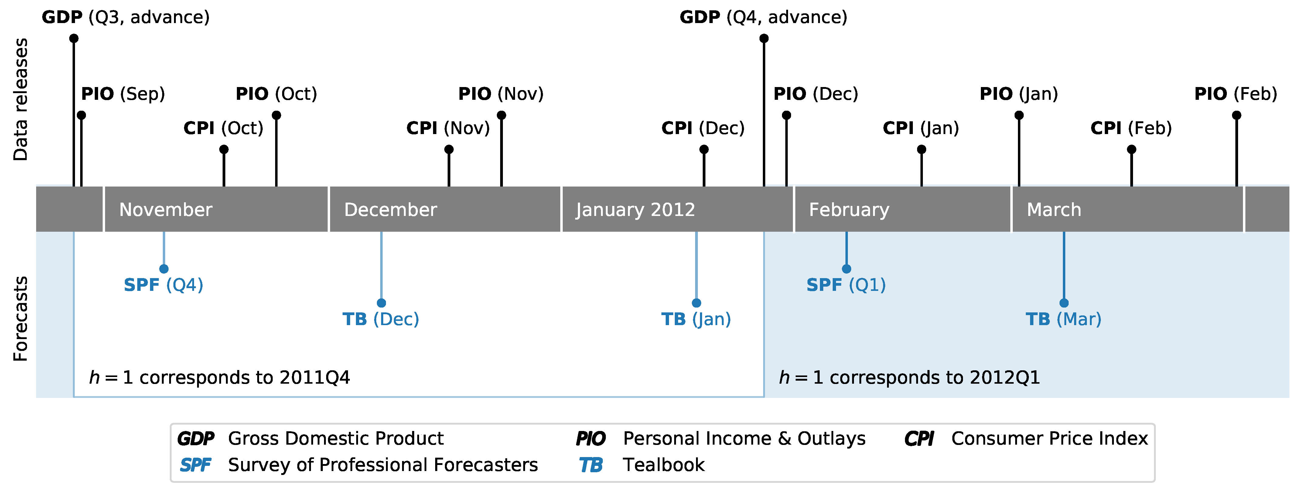
The Survey of Professional Forecasters (SPF) is a quarterly survey published by the Federal Reserve Bank of Philadelphia, with timing based around the release schedule for Gross Domestic Product (GDP) and quarterly PCE prices, which are both part of the National Income and Product Accounts (NIPA).8 In particular, surveys are typically sent to and due to be returned by respondents early in the second month of a given quarter. This is timed to occur shortly after the first—or “advance”—release of the NIPA data for the previous quarter. This timing is illustrated in Figure 3, which shows the evolution of data releases and judgmental forecasts for the end of 2011 and beginning of 2012. For example, the advance release of 2011Q3 NIPA data, annotated as “GDP (Q3, advance)”, occurred on October 27, 2011, and survey responses for the fourth-quarter SPF were due on November 8.
The Federal Reserve Board, meanwhile, produces inflation forecasts as part of the “Tealbook” forecasts that are prepared by staff economists in advance of each of eight annually scheduled Federal Open Markets Committee meetings. While this typically results in two Tealbook forecasts per quarter, they are not synchronized specifically to NIPA data releases, and so timing and data availability can vary between Tealbooks. For example, the advance release of 2011Q4 GDP occurred after the publication of both the December 2011 and January 2012 Tealbooks, both of which were published well after fourth-quarter SPF. Archived Tealbook data is made available by the Federal Reserve Bank of Philadelphia Real-Time Data Research center.
In addition to the quarterly data released as part of the NIPAs, a monthly PCE price index is available as part of the BEA’s Personal Income and Outlays (PIO) release, and the CPI is similarly released monthly by the BLS. Depending on the timing of the SPF and Tealbook releases, this can introduce a difference in the dataset available when these different forecasts were produced. For example, Figure 3 shows that between the 2011Q4 SPF due date and the December 2011 Tealbook, price data for October—the first month of the fourth quarter—was released for both the CPI and PCE measures. More generally, high frequency data that may be relevant for inflation forecasting—such as daily data on oil and gasoline prices—accrues over the course of each quarter. As a result, even though each quarterly PCE release corresponds to one SPF forecast and (typically) two Tealbook forecasts, there is a clear difference in the available information set at the time each forecast was produced. In order to alleviate this difference as much as possible, in our exercise we only consider the forecasts produced for the first Tealbook following each advance GDP release. In the example from Figure 3, we compare the 2011Q4 SPF forecasts against those from the December 2011 Tealbook, and discard those from the January 2012 Tealbook, since the latter incorporates even more additional updated information in comparison to the SPF, while the former Tealbook has an information set relatively more comparable to the SPF.
The model-based forecasts that we consider operate only on a quarterly basis, and as such they do not incorporate monthly-frequency data on prices. To fix the timing, we assume that these models were run on the day of the included Tealbook forecast, although since they are estimated only using data through the previous quarter, the specific timing within the quarter matters only to a little.9 Specifically, in the example from Figure 3, the model-based forecasts that we compare against the 2011Q4 SPF and the December 2011 Tealbook only include data through 2011Q3, based on the vintage available at the time of the December Tealbook’s publication.
3. Forecasting Methodology
Our focus is primarily on the root mean squared error (RMSE) of out-of-sample forecasts for quarterly inflation measured by the PCE price index. Our results are usually shown relative to a benchmark model, where a relative RMSE number less than one indicates improvement compared to the benchmark. Because our source data—both for PCE prices and many of the other variables we use, such as GDP—is subject to potentially large revisions, a real-time forecasting exercise is necessary.10
The data we use is drawn from archived Tealbook databases underlying publicly available Tealbook forecasts and from Alfred (the real-time data repository maintained by the Federal Reserve Bank of St. Louis). The timing of forecasts is as follows: once PCE prices are published through period t, we produce forecasts for each period up to two years ahead ( quarters). The two judgmental forecasts that we consider, however, may already have additional information about the quarter , and so those forecasts at the horizon are more accurately described as nowcasts.
To conduct the out-of-sample forecast evaluation, we estimate all models based on a recursively expanding sample that begins in 1988. As described above, to fix timing we define each forecasting vintage by associating it with a specific Tealbook publication. The first Tealbook in our sample was produced in September 1999, at which time published PCE prices ran through 1999Q2, and so the forecast from our first vintage is for the period 1999Q3. The final vintage of our dataset includes published PCE prices through 2019Q3, so that the final forecast is for the period 2019Q4. This vintage corresponds to the December 2019 Tealbook, although due to the five-year embargo period on Tealbooks, the Tealbook forecasts for that vintage are not yet publicly available. Instead, the final set of Tealbook forecasts that we include in our analysis comes from the December 2014 Tealbook, for which the forecast corresponds to 2014Q4. For this reason, we report results that include Tealbook forecasts but end with the December 2014 Tealbook vintage separately from results that extend through the December 2019 vintage but exclude Tealbook forecasts.
Since PCE price data are revised, there is no single source of true data against which to compare our forecasts. We follow Tulip (2009) and Faust and Wright (2013) in using PCE price inflation as measured in the release two quarters after the reference quarter as the true value from which forecast errors are constructed.
3.1. Model-Based Forecasts
We begin our real-time exercise by constructing forecasts of inflation, denoted , from parametric econometric models. These provide an explicit specification of both included variables and inflation dynamics. Since there are an unlimited number of potential forecasting models to consider, we focus our attention on the classes of models that (a) have been shown to produce competitive inflation forecasts in previous studies, (b) are parsimonious, and (c) most directly speak to the role of additional information in inflation forecasting.11 We present a unifying framework in Equation (4) after introducing the first set of different models employed in this paper.
3.1.1. Autoregressive Model (AR)
The first model we consider has a very simple specification, in which the inflation forecasts are produced from the AR(p) model
We then iteratively apply a one-step-ahead forecast h times to construct the desired forecast . The lag order that we present results for, , was selected using the Bayes Information Criteria over the largest sample period.12 This model is univariate in inflation forecasting, and so includes the least additional information of all models that we consider.13
3.1.2. Inflation Gap Model (AR-Gap)
A useful way to incorporate some additional information while maintaining a parsimonious econometric model is to model inflation as exhibiting short-term fluctuations around some underlying trend, denoted . This requires specification of the inflation trend and an econometric model for modeling the dynamics of the “inflation gap”. The inflation gap, denoted , is the difference between inflation and its trend. Here, we use the Survey of Professional Forecasters forecast of average PCE inflation over the next 10 years as a proxy for trend inflation, while we model the inflation gap as an autoregressive process. Relative to the simpler autoregressive model presented above, this model incorporates additional information from survey forecasts to help pin down the “local mean” of inflation. Specifically, the forecasting model is
We then proceed as in Faust and Wright (2013) by taking the predictions of the gap—the forecasts —and adding back the final observation of the trend to get the implied prediction of inflation. We present results for lag order , the same as for the simple autoregression model above.
3.1.3. Phillips Curve Models
We now explicitly incorporate into our forecasts additional information from macroeconomic variables other than inflation, in the form of an empirical Phillips curve model. This class of models is appealing in that it uses macroeconomic variables to forecast inflation and has links to theoretical models of price-setting. The general form of the Phillips curve models that we consider is
where is an estimate of the inflation trend at time t, is a measure of economic slack at time t, and is a vector of controls. By varying the specifications of the inflation trend, economic slack, and the vector of controls, we can accommodate a wide range of additional information.
As in the construction of the inflation gap model above, we model the inflation trend using long-run inflation expectations from the Survey of Professional Forecasters. Economic slack is modeled as the distance between the unemployment rate and an estimate of the natural rate of unemployment. For all forecasts made through December 2014, we use the Tealbook estimate of the natural rate of unemployment, while for the period January 2015 to the present we use the estimate of the natural rate of unemployment produced by the Congressional Budget Office, since Tealbook estimates from this latter period have not yet been made public. The vector of controls that we include contains relative core import price inflation and relative energy price inflation.14 Note that in this model relative import price inflation captures the impact of international inflation developments on US inflation.15
Forecasts of based on this equation require forecasts of the right-hand-side variables. For results that we report, we apply a random walk forecast for the inflation trend and the forecast from an AR(1) model for the other variables.
As a unifying conceptual framework to think about how the different forecasting models use additional information to forecast inflation, one can consider the following extended version of the Phillips curve model that nests the AR, AR-Gap, and standard Phillips curve models described in the paragraphs above:
When , then the AR model is obtained, while when , and we obtain the AR-Gap model that we will use as our benchmark forecast model in the forecast comparison. Finally, if then we obtain the Phillips curve model discussed above.
3.1.4. Vector Autoregressive Model (VAR)
We also consider forecasts from a Vector Autoregressive Model (VAR) that can be thought of as another extension of the unifying Phillips-Curve framework discussed where the right-hand side variables of the single-equation Phillips curve model are included as endogenous variables rather than conditioning on them.
To facilitate the comparison, we use the same variables as we did in our Phillips curve model. As in the simple univariate autoregression, we estimate the parameters of the vector autoregression and then iteratively apply the one-step-ahead forecast h times. We present results for the lag order 1 selected using the Bayes Information Criteria over the largest sample period.
3.2. Aggregating Forecasts of Disaggregate Inflation
As another extension of the unifying Phillips-Curve framework outlined above, we also produce forecasts of the primary disaggregate series that make up total PCE price inflation and then combine them as a weighted average to forecast the aggregate. Here, our primary focus is on including additional information in the model specification, and we are able to allow different price subcomponents to depend on different macroeconomic variables and to exhibit different dynamics. In particular, we separately make forecasts for core PCE price inflation, food PCE price inflation, and energy PCE price inflation, and then combine them using their relative shares in PCE as weights.
The forecast of core PCE price inflation is based on a Phillips curve model similar to the empirical Phillips Curve model described above. The forecast for food PCE price inflation is also based on a similar Phillips curve model, except that in this case, no control variables are included so that the term with is dropped. Energy PCE price inflation is modeled as , where is oil price inflation. Forecasts are then produced by assuming that oil price inflation follows a random walk. This aggregated forecast approach potentially improves the accuracy of forecasting the aggregate by a reduction in the estimation uncertainty and misspecification.
3.3. Judgmental Forecasts
We include in our forecasting exercise two sets of forecasts that are not based on an explicit forecasting model. Relative to model-based forecasts, these judgmental forecasts are likely based on a much larger information set.
3.3.1. Survey of Professional Forecasters (SPF)
First, we include forecasts based on responses to the Survey of Professional Forecasters (SPF). Since 2007, the SPF has included forecasts of total PCE price inflation at quarterly horizons as well a forecast of average annual inflation over the next ten years, intended to capture expected long-run inflation. To construct forecasts for the horizons , we follow an approach along the lines of that suggested by Faust and Wright (2013) and linearly interpolate between a near-term forecast and a long-term forecast.16 In particular, we set the forecast equal to the SPF forecast for long-run inflation and then linearly interpolate between the and values. In all cases, we use median SPF forecasts. Prior to 2007, the SPF only produced forecasts of consumer price index (CPI) inflation, and so we must use implied forecasts for PCE. As noted earlier, differences in the construction of these two price indices tend to lend an upwards bias to CPI inflation compared to PCE inflation.17 To impute forecasts for PCE price inflation prior to 2007, at each period we start with the CPI forecast provided by the SPF and then subtract the historical wedge (as would have been computed at that time) between published CPI inflation and published PCE price inflation.
3.3.2. Tealbook Forecasts of Federal Reserve Board Staff
Second, we include the forecasts provided in each Tealbook for total PCE price inflation, which are judgmental forecasts produced by staff of the Federal Reserve Board of Governors. Due to the 5-year lag between finalizing the Tealbook and its public release, Federal Reserve Board staff forecasts are only available prior to 2015, and our primary exercise therefore only considers forecasts made through the end of 2014. A secondary exercise expands the sample to include forecasts made through the end of 2019, although it excludes Tealbook forecasts. It should be noted that the Tealbook forecast takes into account that the US is an open economy given the staff discussions and taking on board conditional assumptions, for instance about oil prices and trade.
3.4. Forecast Combination
As a final part of our analysis we include a forecast for PCE price inflation generated by taking a weighted average of the forecasts from the models described above, except excluding the Tealbook forecasts. We consider two methods for generating the forecast combination weights: in the first case (referred to below as “simple” combination), the weights are set equal for each model, while in the second case (referred to below as the “MSE” combination) the weight for a given model at the time t is set to be the inverse of the root mean squared error generated by the model over the preceding 8 quarters. Combining different forecast of the same variable can improve over the best forecast when forecasts are biased in opposite direction.18 Furthermore, the forecast combination method with time-varying weights helps to shed light on the time-varying relative forecast performance of the different models included in the forecast comparison.
4. Results: Forecasting US PCE Inflation in Real Time
We begin by presenting results for our comparison of forecasts of US PCE inflation in real-time for the portion of our sample period for which public Tealbook forecasts are available, 1999Q3–2016Q3, and then discuss the pre- and post-crisis periods for that sample.19 Our focus will be on the root mean square error (RMSE) of our forecasts relative to the AR(1) model in the inflation gap. Our RMSE evaluation is based on quarterly inflation.20 This is also the model that Faust and Wright (2013) use as their benchmark, and we found that it outperforms other candidate benchmarks (such as the AR(1) model in inflation). We have also carried out Diebold-Mariano (DM) tests (see Diebold and Mariano (1995); West (1996); Diebold (2015)) to investigate whether the RMSE improvements over the benchmark model were significant.21
4.1. Real-Time Analysis Including Public Tealbook Forecasts
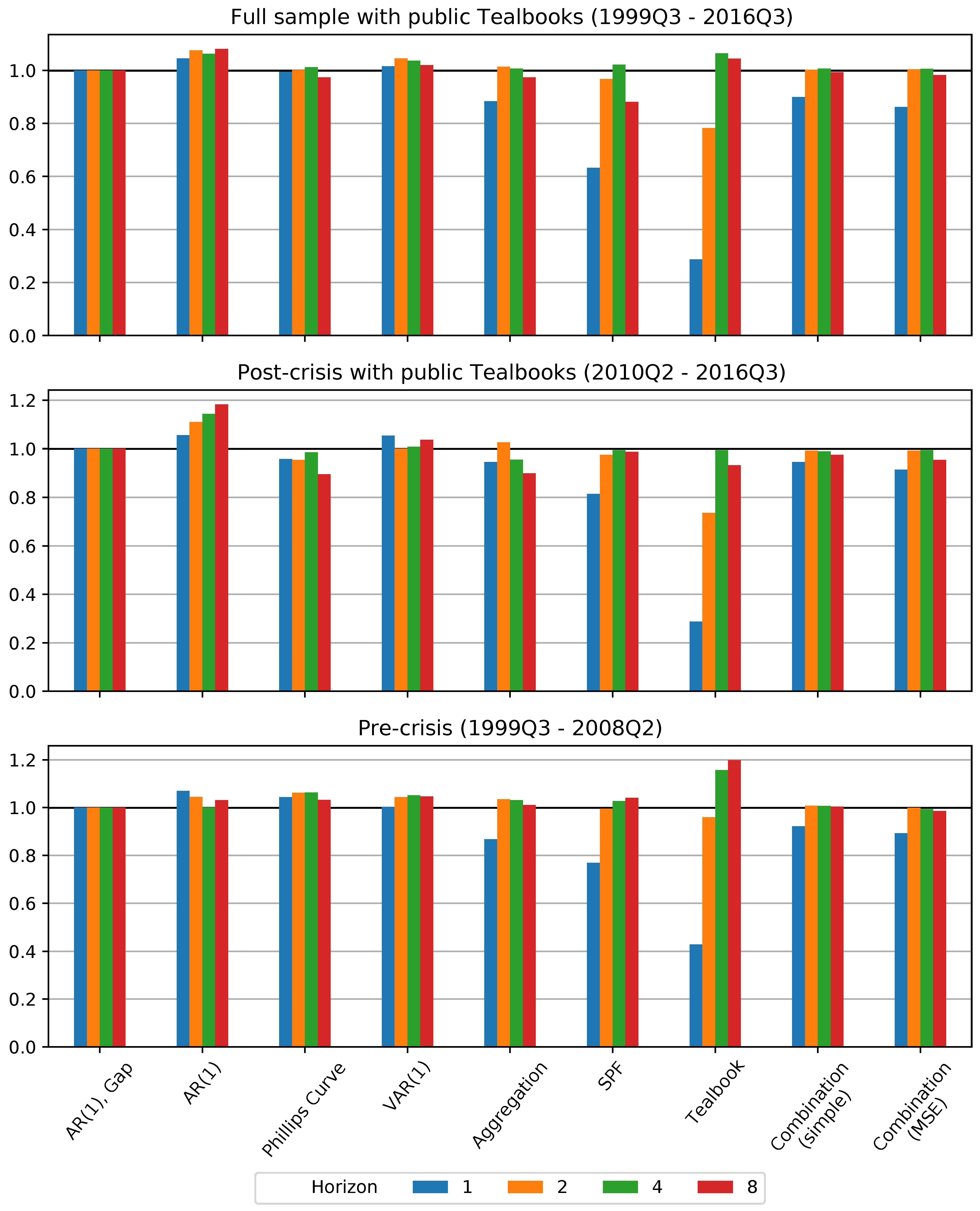
We first consider a comparison of our selected forecast models and methods for the sample period, 1999Q3–2016Q3, where our second source of judgmental forecasts—those produced by the staff of the Federal Reserve Board (FRB) and recorded in Tealbooks—is publicly available. Due to the embargo on recent Tealbooks, for the results in this section we restrict our sample so that the final forecasts were produced in 2014Q4. The relative RMSE results are shown in Figure 4, and the relevant DM test results are presented in Table 1.
A key takeaway over the full sample for which the Tealbook is available is that the autoregressive model in the inflation gap is generally difficult to improve upon except for horizon . Indeed, the model-based forecasts that incorporate specific additional macroeconomic variables—the Phillips curve and vector autoregression—do no better than this benchmark, except for the Phillips curve model during the post-crisis period. However, improvements from some of the forecasting methods we employ, in particular judgmental forecasts, forecast aggregation and forecast combination, do stand out.
First, the aggregated forecast—which forecasts core, food, and energy prices separately before aggregating them to produce the total PCE price inflation forecast—is able to improve on the gap model at the horizon . This is particularly noteworthy since the other forecast methods that improve at this horizon incorporate mixed frequency data (see the discussion of the SPF, Tealbook, and combination models below), while this method does not. The improvements for the aggregated forecast are statistically significant at this horizon, according to DM test results, but not for other horizons.
Second, the SPF forecast shows a dramatic reduction in forecasting error at the horizon . As described above, SPF respondents generally produce this forecast at the beginning of the second month of the quarter being forecasted, and so it can be labeled as a nowcast. Thus, this enhanced forecasting performance reflects both the judgmental expertise of the forecasters and the fact that SPF forecasters have access to a larger information set, including some information about the quarter, when making their forecast. At a horizon of two years ahead () the SPF forecast is also superior to the benchmark, while for horizons and there is little or no improvement in SPF forecast performance over the benchmark. The improvements in forecast performance for are clearly statistically significant for the pre- and post-crisis period, and borderline significant for the full sample period according to the DM test.
Third, the forecasts produced by forecast combination methods show improvements over the benchmark. These include the SPF as one of the constituent forecasts, and their improvement relative to the benchmark at the horizon show that they are able to take advantage of SPF forecast improvements. At the same time, the combination forecasts provide a robust forecast, as they do not degrade as much as the SPF at longer horizons, and always improve over the worst models, including both the AR(1) and VAR(1). Finally, the combination incorporating time-varying weights performs slightly better than the equal-weight counterpart, suggesting that it can be useful to take into account variation over time in forecasting performance. The RMSE improvements of the combination method with time-varying weights over the benchmark model are statistically significant for both 1 quarter and 2 year horizons ( and ).
Finally, the public Tealbook forecasts by Federal Reserve staff provide substantial and statistically significant forecasting improvements at horizons , but do not outperform the benchmark model at the longer horizons. The most conspicuous result is the performance of the nowcast () contained in the Tealbook, even compared to that from the Survey of Professional Forecasters. Although striking, this result likely largely reflects the fact that Federal Reserve staff nowcasts take into account a much larger information set than the models we consider, which include at most a handful of explanatory variables. Although some of this improvement is no doubt due to the use of higher-frequency variables, the Tealbook nowcasts also substantially outperform those of the Survey of Professional Forecasters, who would have had access to similar data, although as noted in Section 2, the Tealbook forecasts have a slightly updated information compared to the SPF forecasts. Altogether, this suggests that Tealbook nowcasts provide an upper bound for forecasting improvements, and shows that even the quite-good SPF nowcasts still have room to improve.
A second notable result from our out-of-sample forecast comparison is the strong improvement of the Tealbook forecast compared to the benchmark model at the horizon – the only forecast to outperform the benchmark at this horizon, although only statistically significant on a 15 percent significance level. One explanation for this result is, as noted by Faust and Wright (2013), that a good forecast for can help improve the forecast for . This suggests that there are gains still available in near-term inflation forecasting (even beyond those gained by using higher-frequency data to produce nowcasts), either from additional data with predictive power or from improved models.
4.2. Pre- vs. Post-Crisis Analysis Including Public Tealbooks
The global financial crisis and subsequent Great Recession substantially disrupted the US economy; this raises several questions relevant for inflation forecasting. First, forecasting errors made during the crisis—a time in which inflation was quite volatile—might be influencing our results. Second, a structural break might have occurred in inflation dynamics, so that forecasting methods or sources of information that improved forecast accuracy in comparison to the benchmark model prior to the crisis might not provide similarly accurate forecasts after the crisis. For instance, it might be argued that the slow labor market recovery following the global financial crisis (see Figure 1) was evidence of an altered economic climate compared to the pre-crisis period, with implications for inflation. To address these issues, we consider subsample analyses of the pre- and post-crisis periods, with results shown in the middle and lower panel of Figure 4.
Comparison of the forecasting performance in the pre- and post-crisis periods suggests that our primary qualitative results described for the full sample agree with those from the pre-crisis period, but begin to break down during the post-crisis period as many models outperform the benchmark at both short and long horizons in RMSE terms.
These results suggest that there can be room for the use of additional information in improving inflation forecasting, particularly in the post-crisis period, and especially at very short and very long horizons.22 Moreover, we are able to find several different methods of incorporating additional information into econometric models that produce these improvements. Notably, and unlike in previous work, here we find that Phillips curve models can still improve on simple forecasting models when forecasting inflation in some situations.
To summarize the results of the sample and sub-samples that include the public Tealbook forecasts: we find that the methods that include richer information sets (compared to simple forecasts based on just one univariate or multivariate forecast model) all significantly improve over the benchmark inflation gap model for the full sample including public Tealbooks and the pre-crisis period at the shortest horizon. These models include the aggregation, the combination methods—including both the simple average and the time-varying MSE-weighted combination—as well as the judgmental forecasts—including both the SPF and Tealbook forecasts.
In the post-crisis period including public Tealbooks, we continue to find that the time-varying, MSE-weighted combination and both judgmental forecasts improve significantly over the benchmark model, while the improvements of the aggregation method and simple combination are not significant at the short horizon. Meanwhile, the aggregation forecast and the time-varying, MSE-weighted combination forecast both significantly improve over the benchmark at the 2-year horizon.
4.3. Full Sample through 2019
To investigate whether our results for the baseline sample period (the period that includes publicly available Tealbooks) also hold for an extended sample period, we compare the forecasts from the forecast models and methods other than the Tealbook for the full sample including recent history up to 2019 as well as the post-crisis period including these more recent years. The results for the full sample are shown in the upper panel of Figure 5, while the results for the post-crisis period up to 2019 are shown in the lower panel. Results for the DM tests are shown in Table 2.
It is noteworthy that there is little change in the relative forecast performance of the models when adding five additional years. For the full sample, the inflation gap is still difficult to improve upon, apart from the horizon where the SPF, aggregation, and combination methods provide a significantly better forecast than the benchmark model, and the horizon , where the time-varying MSE-weighted combination method improves over the benchmark. For the post crisis period through 2019 we get the same results, except that the aggregated forecast and the Phillips Curve model significantly improve over the benchmark for while the time-varying MSE-weighted combination method improvement is not signficant.
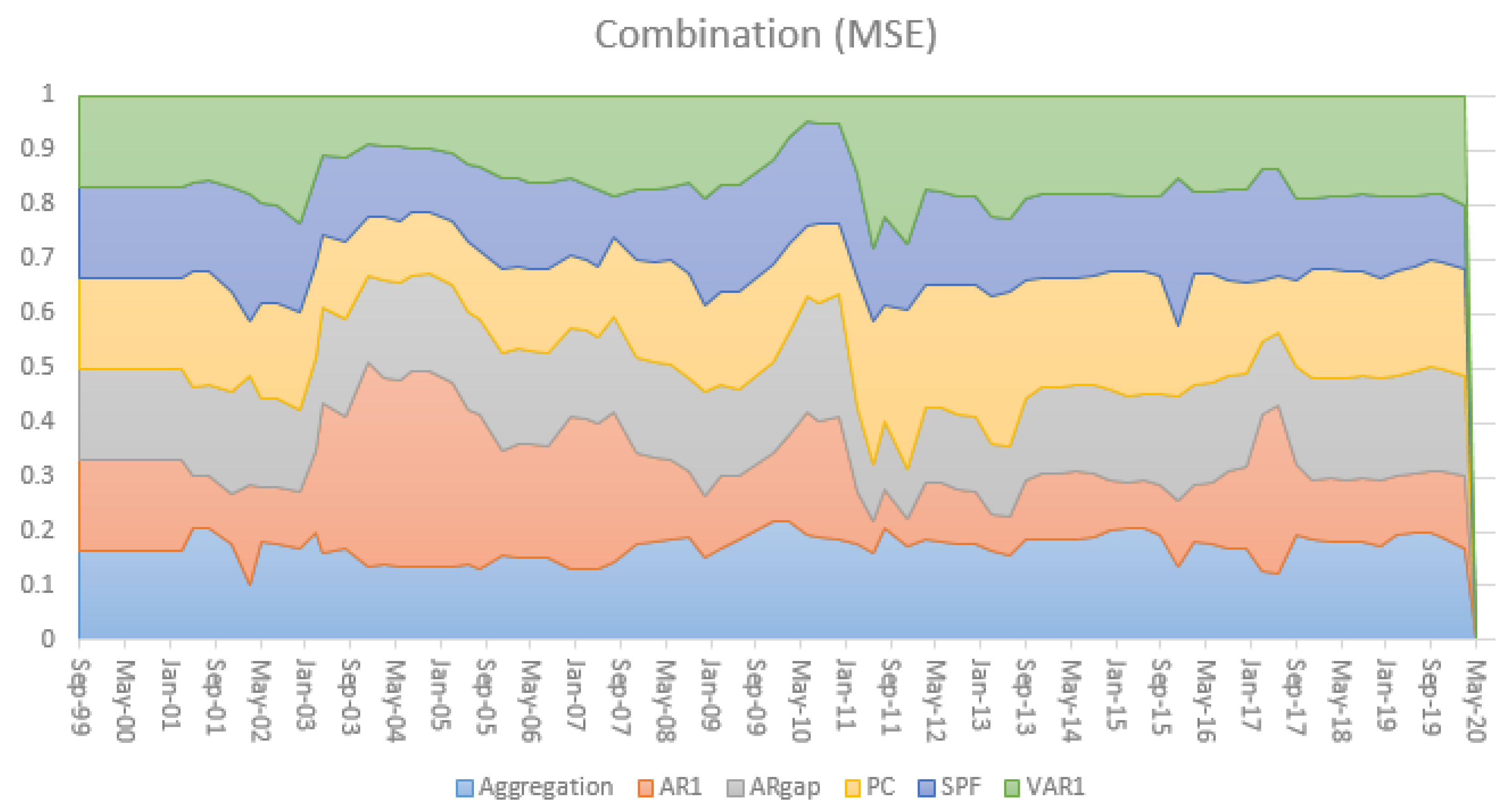
The time-varying relative performance in terms of MSE is nicely illustrated in Figure 6 and Figure 7 for horizons and , respectively. It also illustrates the relevance of the larger information set incorporated in the SPF for in episodes with higher uncertainty and volatility, for instance during the Global Financial Crisis.
4.4. Summary of Results
Overall, there are two main takeaways that we think are worth highlighting: First, the time-varying MSE-weighted combination method consistently and significantly improves on the benchmark across different samples for horizons of 1 quarter and 8 quarters (the latter except for the post-crisis full sample period, where the aggregation method is better). Second, for the nowcast it should be noted that the SPF and Tealbook forecasts improve significantly over the benchmark, so the additional information used in those forecasts helps improving the prediction accuracy.
5. Remarks
- (1)
- Forecast encompassing, forecast combination and forecast accuracy tests: Having the smallest RMSE comparisons of a set of forecasts is a necessary but not sufficient condition for forecast encompassing (see Ericsson (1992)). The concept of forecast encompassing has been proposed by Chong and Hendry (1986) and can be tested by investigating whether the forecast of the alternative forecast model can explain the forecast error of a benchmark forecast model of interest. We explore forecast combination as one possible forecast method. Forecast combination is closely related to the concept of forecast encompassing. Evidence that forecast combination of two forecasting models provides smaller RMSE than the benchmark model implies that the benchmark forecast does not encompass the alternative model forecast. Our result that forecast combination does improve over simple benchmark models and also over Phillips curve models does suggest that some of the alternative models contain additional predictive content. This is confirmed by our result of the Diebold and Mariano test that forecast combination significantly outperforms the simple benchmark model for horizons of one quarter and two years across all samples and most pre- and post-crisis subsamples. One extension for further research would be to apply the test suggested by Hubrich and West (2010) to compare small nested model sets via adjust MSFEs relevant to some of the comparisons, that can be viewed as a forecast encompassing test for small nested model sets.
- (2)
- Other models We have included (but do not present) in our forecast comparison a random walk model that has often been used as a benchmark model in the literature. We also considered forecasts based on an AR(1) model estimated with a rolling estimation window instead of a recursively expanding estimation window. We find that the rolling window AR model performs slightly better than the benchmark and all the other models for a one year horizon for the post-crisis period that includes the published Tealbook as well as the full post-crisis period, and performs better than the benchmark for most horizons for the pre-crisis period. Other than these few instances, neither of these models does outperform our benchmark inflation gap model in RMSE terms except at very few horizons and in those cases the improvement was negligible and in any case clearly outperformed by our best forecasting methods.
- (3)
- RMSEs comparisons: We compare the different forecast models and methods in terms of RMSE. As Clements and Hendry (1993) have pointed out, RMSE are not invariant to certain transformations. For example, different transformations (first differences or annual differences) might affect the RMSE ranking of the forecast models. We have focused on the forecast performance for quarterly inflation, and note that the RMSE based forecast comparison might be different for annual inflation. However, we choose out-of-sample RMSE comparisons because parameter estimation uncertainty and structural breaks often imply that good in-sample fit does not translate into out-of-sample forecasting (see, e.g., Clements and Hendry (1998); Giacomini and Rossi (2009)).
- (4)
- SPF It should be noted that the SPF is itself an average (or a median) and so may already benefit from any aggregation effects due to differentially misspecified models or methods by forecasters in the sample.
6. Conclusions
In this paper, we perform a real-time forecasting exercise, focusing on price inflation as measured by the personal consumption expenditures (PCE) chain-type price index that is most relevant for monetary policy decisions. We investigate whether and how additional information—additional macroeconomic variables, expert judgment, or forecast combination—can improve forecast accuracy. We analyze pre- and post-crisis performance of different inflation forecasting models as well as judgmental forecasts from the SPF and Tealbook. We show which forecasting methods are most useful before, during, and after the global financial crisis, and so aim to shed light on which methods are most promising for constructing and robustifying inflation forecasts. Our analysis is also relevant in light of the current crisis that has posed challenges for forecasting, given the unprecedented nature of the pandemic. Hence, strategies to robustify forecasts, such as the ones we have considered here, are likely to be increasingly important.
Our results provide interesting new insights for inflation forecasting from recent episodes, while some of our results confirm previous literature. Our key finding is that while simple models remain generally hard to beat, careful introduction of additional information can improve forecasts, particularly in the post-crisis period. Three types of additional information stand out as useful. First, forecast combination of different models for overall inflation are competitive and robustify against bad forecasts. Second, aggregating forecasts of inflation components can improve performance compared to forecasting the aggregate directly, suggesting that there are gains to be had from the careful specification of the dynamics of disaggregate inflation series. Finally, the large information set available to professional forecasters and the Federal Reserve Board staff can substantially improve forecasting performance, especially at short horizons, suggesting that multivariate models, including those capable of handling large data sets, can play an important role in inflation forecasting.
-4.5cm0cm [custom]
Author Contributions
Conceptualization, C.F. and K.H.; Methodology, C.F. and K.H.; Software, C.F. and K.H.; Formal Analysis, C.F. and K.H.; Writing and Original Draft Preparation, C.F. and K.H.; Writing Review and Editing, C.F. and K.H. All authors have read and agreed to the published version of the manuscript.
Funding
This research received no external funding.
Institutional Review Board Statement
Not applicable.
Informed Consent Statement
Not applicable.
Data Availability Statement
Not applicable.
Acknowledgments
The views expressed in this paper are those of the authors and do not necessarily reflect those of the Federal Reserve Board or the Federal Reserve System or its staff. We thank Neil Ericsson and two anonymous referees for useful suggestions as well as participants of the International Association for Applied Econometrics 2019 conference, the Conference on Computational and Financial Econometrics 2019, the International Forecasting Symposium 2021, and the Joint Statistical Meetings 2021 for helpful comments.
Conflicts of Interest
The authors declare no conflict of interest.
| 1 | |
| 2 | |
| 3 | While the CPI and PCE price index share a similar low-frequency evolution, differences in formula, weight, and scope—as discussed in, for example, McCully et al. (2007)—can result in persistent differences in measured inflation. One commonly noted implication of the formula effect is that the CPI—which employs a Laspeyres index concept—is slower to accommodate consumer substitution between goods, and so tends to increase at a faster pace than the PCE price index. |
| 4 | Indeed, the CPI was the only measure of inflation explicitly included in the projections of Federal Reserve Banks and Board members produced as part of the semi-annual Monetary Policy Report (MPR) to Congress during the period 1992–1999. We thank Neil Ericsson for pointing this out to us. |
| 5 | While our econometric forecasting models are specified at the quarterly frequency and so do not take this higher-frequency information into account, we include judgmental forecasts from the Survey of Professional Forecasters and Federal Reserve Board Tealbooks that do incorporate this information. Recent work on mixed frequency econometric models that can be used for the purpose of “nowcasting” inflation includes Modugno (2013) and Knotek and Zaman (2017). |
| 6 | It is worth noting that the raw price data that underlies both of these measures is known to be subject to measurement error, as documented in Shoemaker (2011) and Eichenbaum et al. (2014). While we are not able to correct for these errors, they primarily affect the most disaggregate inflation series, and are less of a concern for the high-level aggregates that we use for forecasting. |
| 7 | Indeed, the MPR (see Note 6) replaced overall PCE prices with core PCE prices in 2004, and the FOMC Summary of Economic Projections, introduced in 2007, includes both measures. |
| 8 | Croushore and Stark (2019) provide a recent overview of the details of this survey. |
| 9 | For example, if the estimate of the history of the unemployment gap was revised during a given quarter, then the specific timing of the forecast could have a small effect on models that include that variable. |
| 10 | Measurement errors to a particular variable might be systematic, and one line of research has distinguished between “news” and “noise” in the revision process of data. In practice, data revisions are difficult to model. |
| 11 | Alternatively, we could have considered to start from a general unrestricted model using a general-to-specific model selection strategy involving multiple path searches, encompassing tests and a set of diagnostic tests, as has been advocated by David Hendry and is implemented in Autometrics (see, e.g., Doornik (2009)). More generally, model selection can be considered as a strategy where smaller models are tested against more general model. Our comparison of forecasting models and methods using a smaller information set with models and methods using larger information sets is in that spirit. See Castle et al. (2021). |
| 12 | We also examined both the Bayes Information Criteria and the Akaike Information Criteria in real time. Our selected lag order is competitive across most of the sample period for both criteria, and it is the model most preferred by the Bayes criteria since about 2009. |
| 13 | We also examined other common parsimonious univariate models, including the random walk forecast and the model of Atkeson and Ohanian (2001). We report results for the AR(p) model since it exhibited better forecasting performance in our sample. |
| 14 | There are a huge number of empirical Phillips curve specifications that have been considered in the literature, and although we report results for only one specification, we considered many alternatives. For example, we considered models with the inflation trend derived from different survey measures or from the Federal Reserve Board staff forecasts and for economic slack we considered various measures of both the unemployment gap and output gap. |
| 15 | In the aggregated model presented below we model energy inflation as a function of oil prices to capture a different dimension of international influences on inflation. |
| 16 | The good performance of this interpolation approach noted by Faust and Wright (2013) suggests that it would also be interesting to apply it using our model-based forecasts in place of the SPF forecasts, although we leave this for future work. |
| 17 | This feature is discussed in Note 6 and can be seen in Figure 2. |
| 18 | Note that combining forecasts with overlapping information content can also lead to improved MSFE due to differentially mis-specified forecasts. Comparing in-sample to out-of-sample weighting in terms of equal weights versus MSE weights would be an interesting extension |
| 19 | Note that this sample period describes the included forecast periods. While the final public Tealbook is from December 2014, its forecast corresponds to 2016Q3. |
| 20 | Note that the ranking between the different forecasting models and methods might differ based on a different transformation, such as annual inflation. |
| 21 | Statements in the text refer to the 10 percent significance level. |
| 22 | Indeed, these were the horizons emphasized as most important by Faust and Wright (2013). |
References
- Atkeson, Andrew, and Lee E. Ohanian. 2001. Are Phillips curves useful for forecasting inflation? Federal Reserve Bank of Minneapolis Quarterly Review 25: 2–11. [Google Scholar] [CrossRef] [Green Version]
- Castle, Jennifer L., Jurgen A. Doornik, and David F. Hendry. 2021. Selecting a model for forecasting. Econometrics 9: 26. [Google Scholar] [CrossRef]
- Chong, Yock Y., and David F. Hendry. 1986. Econometric evaluation of linear macroeconomic models. Review of Economic Studies 53: 671–90. [Google Scholar] [CrossRef]
- Clements, Michael. P., and David F. Hendry. 1993. On the limitations of comparing mean square forecast errors. Journal of Forecasting 12: 617–37. [Google Scholar] [CrossRef]
- Clements, Michael. P., and David F. Hendry. 1998. Forecasting Economic Time Series. Cambridge: Cambridge University Press. [Google Scholar]
- Croushore, Dean, and Tom Stark. 2019. Fifty years of the survey of professional forecasters. Economic Insights 4: 1–11. [Google Scholar]
- Diebold, Francis X. 2015. Comparing predictive accuracy, twenty years later: A personal perspective on the use and abuse of Diebold—Mariano tests. Journal of Business and Economic Statistics 33: 1–9. [Google Scholar] [CrossRef] [Green Version]
- Diebold, Francis X., and Roberto. S. Mariano. 1995. Comparing predictive accuracy. Journal of Business and Economic Statistics 13: 253–63. [Google Scholar]
- Doornik, Jurgen A. 2009. The Methodology and Practice of Econometrics: A Festschrift in Honour of David F. Hendry. Edited by Jennifer Castle and Neil Shephard. Oxford: Oxford University Press, pp. 88–21. [Google Scholar]
- Eichenbaum, Martin, Nir Jaimovich, Sergio Rebelo, and Josephine Smith. 2014. How frequent are small price changes? American Economic Journal: Macroeconomics 6: 137–55. [Google Scholar] [CrossRef] [Green Version]
- Ericsson, Neil R. 1992. Parameter constancy, mean square forecast errors, and measuring forecast performance: An exposition, extensions, and illustration. Journal of Policy Modeling 14: 465–95. [Google Scholar] [CrossRef] [Green Version]
- Faust, Jon, and Jonathan H. Wright. 2013. Forecasting inflation. In Handbook of Economic Forecasting. Amsterdam: Elsevier, vol. 2, pp. 2–56. [Google Scholar]
- Giacomini, Raffaella, and Barbara Rossi. 2009. Detecting and predicting forecast breakdowns. The Review of Economic Studies 76: 669–705. [Google Scholar] [CrossRef] [Green Version]
- Granger, Clive W. J. 1987. Implications of aggregation with common factors. Econometric Theory 3: 208–22. [Google Scholar] [CrossRef]
- Hendry, David F., and Kirstin Hubrich. 2011. Combining disaggregate forecasts or combining disaggregate information to forecast an aggregate. Journal of Business & Economic Statistics 29: 216–27. [Google Scholar]
- Hendry, David F., and Michael P. Clements. 2004. Pooling of forecasts. The Econometrics Journal 7: 1–31. [Google Scholar] [CrossRef] [Green Version]
- Hubrich, Kirstin. 2005. Forecasting euro area inflation: Does aggregating forecasts by HICP component improve forecast accuracy? International Journal of Forecasting 21: 119–36. [Google Scholar] [CrossRef] [Green Version]
- Hubrich, Kirstin, and Frauke Skudelny. 2017. Forecast combination for euro area inflation: A cure in times of crisis? Journal of Forecasting 36: 515–40. [Google Scholar] [CrossRef] [Green Version]
- Hubrich, Kirstin, and Kenneth West. 2010. Forecast evaluation of small nested modelsets. Journal of Applied Econometrics 25: 574–94. [Google Scholar] [CrossRef] [Green Version]
- Knotek, Edward S., and Saeed Zaman. 2017. Nowcasting US headline and core inflation. Journal of Money, Credit and Banking 49: 931–68. [Google Scholar] [CrossRef]
- Lütkepohl, Helmut. 1984. Forecasting contemporaneously aggregated vector ARMA processes. Journal of Business & Economic Statistics 2: 201–14. [Google Scholar]
- McCully, Clinton P., Brian C. Moyer, and Kenneth J. Stewart. 2007. Comparing the consumer price index and the personal consumption expenditures price index. Survey of Current Business 87: 26–33. [Google Scholar]
- Modugno, Michele. 2013. Now-casting inflation using high frequency data. International Journal of Forecasting 29: 664–75. [Google Scholar] [CrossRef] [Green Version]
- Powell, Jerome. 2018. Monetary Policy and Risk Management at a Time of Low Inflation and Low Unemployment. Paper presented at the “Revolution or Evolution? Reexamining Economic Paradigms” 60th Annual Meeting of the National Association for Business Economics, Boston, MA, USA, September 29–October 2. [Google Scholar]
- Shoemaker, Owen J. 2011. Variance Estimates for Price Changes in the Consumer Price Index. Bureau of Labor Statistics Report. Washington, DC: Bureau of Labor Statistics. [Google Scholar]
- Stock, James H., and Mark W. Watson. 2007. Why has US inflation become harder to forecast? Journal of Money, Credit and Banking 39: 3–33. [Google Scholar] [CrossRef] [Green Version]
- Stock, James H., and Mark W. Watson. 2016. Core inflation and trend inflation. Review of Economics and Statistics 98: 770–84. [Google Scholar] [CrossRef]
- Tulip, Peter. 2009. Has the economy become more predictable? changes in Greenbook forecast accuracy. Journal of Money, Credit and Banking 41: 1217–31. [Google Scholar] [CrossRef]
- West, Kenneth D. 1996. Asymptotic inference about predictive ability. Econometrica 64: 1067–84. [Google Scholar] [CrossRef]
- Yellen, Janet L. 2015. Inflation Dynamics and Monetary Policy. Amherst: Philip Gamble Memorial Lecture, University of Massachusetts. [Google Scholar]
Figure 1.
Historical US unemployment, wage inflation, and price inflation.

Figure 2.
Annualized quarterly inflation rates for various price indexes using data from the 2020Q3 vintage.
Figure 2.
Annualized quarterly inflation rates for various price indexes using data from the 2020Q3 vintage.

Figure 3.
Example of data release and forecast timing for the period November 2011 through March 2012.
Figure 3.
Example of data release and forecast timing for the period November 2011 through March 2012.

Figure 4.
Relative RMSE of selected inflation forecasts, sample including public Tealbooks.

Figure 5.
Relative RMSE of selected inflation forecasts, full sample.

Figure 6.
MSE based time-varying weights in combination forecast, .

Figure 7.
MSE based time-varying weights in combination forecast, .


Table 1.
Forecast comparison, sample including public Tealbooks.
| Horizon | AR(1), Gap | AR(1) | Phillips Curve | VAR(1) | Aggregation | SPF | Tealbook | Combination | |
|---|---|---|---|---|---|---|---|---|---|
| Simple | MSE | ||||||||
| Full sample with public Tealbooks (1999Q3–2016Q3) | |||||||||
| 1 | 1.65 | 1.73 | 1.65 | 1.68 | 1.46 | 1.05 | 0.47 | 1.49 | 1.43 |
| – | −1.75 | 0.23 | −0.71 | 1.81 * | 1.57 | 2.03 * | 1.68 * | 1.73 * | |
| – | [0.086] | [0.388] | [0.310] | [0.078] | [0.117] | [0.051] | [0.097] | [0.090] | |
| 2 | 1.73 | 1.86 | 1.73 | 1.81 | 1.75 | 1.67 | 1.35 | 1.73 | 1.74 |
| – | −1.86 | −0.08 | −1.66 | −0.63 | 0.90 | 1.49 | −0.23 | −0.39 | |
| – | [0.070] | [0.398] | [0.100] | [0.326] | [0.265] | [0.132] | [0.388] | [0.370] | |
| 4 | 1.67 | 1.77 | 1.69 | 1.73 | 1.68 | 1.70 | 1.77 | 1.68 | 1.68 |
| – | −1.72 | −0.44 | −1.68 | −0.31 | −1.01 | −1.34 | −0.73 | −0.48 | |
| – | [0.092] | [0.362] | [0.097] | [0.380] | [0.240] | [0.163] | [0.306] | [0.356] | |
| 8 | 1.71 | 1.85 | 1.67 | 1.75 | 1.67 | 1.51 | 1.79 | 1.70 | 1.68 |
| – | −2.33 | 1.03 | −0.51 | 1.40 | 0.96 | −0.81 | 0.96 | 2.00 * | |
| – | [0.026] | [0.235] | [0.350] | [0.150] | [0.251] | [0.287] | [0.252] | [0.054] | |
| Post-crisis with public Tealbooks (2010Q2–2016Q3) | |||||||||
| 1 | 1.11 | 1.17 | 1.07 | 1.17 | 1.05 | 0.91 | 0.32 | 1.05 | 1.02 |
| – | −1.23 | 0.46 | −0.49 | 1.41 | 2.77 ** | 4.51 ** | 1.61 | 1.95 * | |
| – | [0.187] | [0.359] | [0.353] | [0.147] | [0.009] | [0.000] | [0.109] | [0.059] | |
| 2 | 1.43 | 1.59 | 1.37 | 1.43 | 1.47 | 1.40 | 1.05 | 1.42 | 1.42 |
| – | −2.07 | 0.54 | −0.00 | −0.53 | 0.39 | 1.25 | 0.22 | 0.19 | |
| – | [0.047] | [0.345] | [0.399] | [0.347] | [0.370] | [0.183] | [0.389] | [0.391] | |
| 4 | 1.35 | 1.54 | 1.33 | 1.36 | 1.29 | 1.34 | 1.34 | 1.33 | 1.34 |
| – | −2.36 | 0.16 | −0.10 | 0.94 | 0.13 | 0.05 | 0.33 | 0.13 | |
| – | [0.025] | [0.394] | [0.397] | [0.257] | [0.396] | [0.399] | [0.378] | [0.396] | |
| 8 | 1.40 | 1.66 | 1.25 | 1.45 | 1.26 | 1.38 | 1.31 | 1.37 | 1.34 |
| – | −4.15 | 2.01 * | −0.36 | 3.55 ** | 0.57 | 0.62 | 1.43 | 1.86 * | |
| – | [0.000] | [0.053] | [0.374] | [0.001] | [0.339] | [0.328] | [0.143] | [0.070] | |
| Pre-crisis (1999Q3–2008Q2) | |||||||||
| 1 | 1.30 | 1.39 | 1.36 | 1.31 | 1.13 | 1.00 | 0.56 | 1.20 | 1.16 |
| – | −1.50 | −1.95 | −0.09 | 2.54 ** | 1.96 * | 3.28 ** | 2.44 ** | 2.54 ** | |
| – | [0.129] | [0.060] | [0.397] | [0.016] | [0.058] | [0.002] | [0.021] | [0.016] | |
| 2 | 1.31 | 1.37 | 1.39 | 1.37 | 1.35 | 1.30 | 1.26 | 1.32 | 1.31 |
| – | −0.58 | −1.65 | −1.72 | −0.64 | 0.06 | 0.38 | −0.56 | 0.05 | |
| – | [0.338] | [0.102] | [0.091] | [0.325] | [0.398] | [0.371] | [0.342] | [0.398] | |
| 4 | 1.31 | 1.31 | 1.39 | 1.38 | 1.35 | 1.34 | 1.51 | 1.32 | 1.30 |
| – | −0.02 | −1.53 | −1.72 | −0.72 | −0.53 | −1.53 | −0.49 | 0.44 | |
| – | [0.399] | [0.124] | [0.091] | [0.307] | [0.346] | [0.123] | [0.353] | [0.362] | |
| 8 | 1.45 | 1.50 | 1.50 | 1.52 | 1.47 | 1.51 | 1.74 | 1.46 | 1.43 |
| – | −0.33 | −0.63 | −0.85 | −0.24 | −2.42 | −1.75 | −0.33 | 1.81 * | |
| – | [0.378] | [0.326] | [0.279] | [0.388] | [0.022] | [0.086] | [0.378] | [0.077] | |
Note: this table reports forecast performance and comparison information for nine forecasting models, four forecast horizons, and three subsamples. For each model / horizon / subsample combination, we report three values: the root mean square forecasting error, the test statistic from a Diebold-Mariano test against the baseline “AR(1), gap” model, and the associated p-value. Cases in which the root mean square error is significantly lower than the baseline model at the 10 and 5 percent significance levels are denoted with * or **, respectively.
Table 2.
Forecast comparison, full sample.
| Horizon | AR(1), Gap | AR(1) | Phillips Curve | VAR(1) | Aggregation | SPF | Tealbook † | Combination | |
|---|---|---|---|---|---|---|---|---|---|
| Simple | MSE | ||||||||
| Full sample (1999Q3–2019Q4) | |||||||||
| 1 | 1.53 | 1.61 | 1.52 | 1.56 | 1.34 | 0.95 | – | 1.38 | 1.31 |
| – | −2.40 | 0.39 | −0.76 | 2.16 ** | 1.81 * | – | 1.91 * | 1.98 * | |
| – | [0.023] | [0.369] | [0.298] | [0.039] | [0.078] | – | [0.065] | [0.056] | |
| 2 | 1.56 | 1.68 | 1.56 | 1.62 | 1.58 | 1.51 | – | 1.56 | 1.56 |
| – | −2.34 | 0.02 | −1.57 | −0.75 | 0.77 | – | −0.32 | −0.49 | |
| – | [0.026] | [0.399] | [0.117] | [0.301] | [0.297] | – | [0.379] | [0.354] | |
| 4 | 1.52 | 1.63 | 1.53 | 1.57 | 1.54 | 1.56 | – | 1.53 | 1.53 |
| – | −2.13 | −0.39 | −1.51 | −0.50 | −1.18 | – | −0.91 | −0.66 | |
| – | [0.042] | [0.369] | [0.127] | [0.352] | [0.199] | – | [0.263] | [0.322] | |
| 8 | 1.57 | 1.70 | 1.53 | 1.60 | 1.53 | 1.40 | – | 1.56 | 1.55 |
| – | −2.46 | 0.99 | −0.52 | 1.29 | 0.93 | – | 0.81 | 1.67 * | |
| – | [0.019] | [0.244] | [0.349] | [0.173] | [0.258] | – | [0.288] | [0.100] | |
| Post-crisis (2010Q2–2019Q4) | |||||||||
| 1 | 1.10 | 1.17 | 1.06 | 1.13 | 0.96 | 0.75 | – | 1.00 | 0.95 |
| – | −2.36 | 0.78 | −0.60 | 2.26 ** | 2.49 ** | – | 2.65 ** | 3.06 ** | |
| – | [0.025] | [0.294] | [0.334] | [0.031] | [0.018] | – | [0.012] | [0.004] | |
| 2 | 1.16 | 1.31 | 1.11 | 1.15 | 1.19 | 1.15 | – | 1.16 | 1.16 |
| – | −3.10 | 0.71 | 0.12 | −0.76 | 0.15 | – | 0.14 | 0.09 | |
| – | [0.003] | [0.310] | [0.396] | [0.299] | [0.395] | – | [0.395] | [0.397] | |
| 4 | 1.13 | 1.31 | 1.11 | 1.13 | 1.11 | 1.14 | – | 1.13 | 1.13 |
| – | −3.03 | 0.22 | −0.04 | 0.52 | −0.25 | – | 0.08 | −0.10 | |
| – | [0.004] | [0.389] | [0.399] | [0.348] | [0.386] | – | [0.398] | [0.397] | |
| 8 | 1.22 | 1.44 | 1.11 | 1.26 | 1.11 | 1.21 | – | 1.19 | 1.17 |
| – | −3.80 | 1.79 * | −0.37 | 2.74 ** | 0.08 | – | 1.13 | 1.42 | |
| – | [0.000] | [0.080] | [0.373] | [0.009] | [0.398] | – | [0.210] | [0.145] | |
Note: this table reports forecast performance and comparison information for nine forecasting models, four forecast horizons, and two subsamples. For each model / horizon / subsample combination, we report three values: the root mean square forecasting error, the test statistic from a Diebold-Mariano test against the baseline “AR(1), gap” model, and the associated p-value. Cases in which the root mean square error is significantly lower than the baseline model at the 10 and 5 percent significance levels are denoted with * or **, respectively. See Table 1 for pre-crisis comparisons. Results for Tealbook forecasts are unavailable for the full sample due to their 5-year embargo period.
Publisher’s Note: MDPI stays neutral with regard to jurisdictional claims in published maps and institutional affiliations. |
© 2021 by the authors. Licensee MDPI, Basel, Switzerland. This article is an open access article distributed under the terms and conditions of the Creative Commons Attribution (CC BY) license (https://creativecommons.org/licenses/by/4.0/).
Share and Cite
MDPI and ACS Style
Fulton, C.; Hubrich, K. Forecasting US Inflation in Real Time. Econometrics 2021, 9, 36. https://doi.org/10.3390/econometrics9040036
AMA Style
Fulton C, Hubrich K. Forecasting US Inflation in Real Time. Econometrics. 2021; 9(4):36. https://doi.org/10.3390/econometrics9040036
Chicago/Turabian StyleFulton, Chad, and Kirstin Hubrich. 2021. "Forecasting US Inflation in Real Time" Econometrics 9, no. 4: 36. https://doi.org/10.3390/econometrics9040036
Note that from the first issue of 2016, this journal uses article numbers instead of page numbers. See further details here.