Jointly Modeling Male and Female Labor Participation and Unemployment

Abstract

The COVID-19 pandemic resulted in the most abrupt changes in U.S. labor force participation and unemployment since the Second World War, with different consequences for men and women. This paper models the U.S. labor market to help to interpret the pandemic’s effects. After replicating and extending Emerson’s (2011) model of the labor market, we formulate a joint model of male and female unemployment and labor force participation rates for 1980–2019 and use it to forecast into the pandemic to understand the pandemic’s labor market consequences. Gender-specific differences were particularly large at the pandemic’s outset; lower labor force participation persists.

1. Introduction

The COVID-19 pandemic resulted in the largest change in U.S. labor force participation and unemployment since the Second World War. As the economy recovers from the pandemic-induced recession, macroeconomic policy has focused on understanding changes in the labor market. Fed Chair Powell noted in their November 2021 post-FOMC press conference that the Federal Reserve’s mandate of maximum employment has become much harder to assess, as “people are staying out of the labor market because of caretaking, [and] because of fear of COVID to a significant extent”. This highlights the importance of examining gender-specific unemployment and labor force participation rates.

Previous research shows that, while labor force participation and unemployment rates move together over time, there are important differences between men’s and women’s roles in the the labor force; see Emerson (2011) and Kleykamp and Wan (2014). Furthermore, while labor market dynamics were stable in past decades, they appear to have changed in the pandemic-induced recession, which has been called a “she-cession”, in which job losses and burdens initially fell disproportionally on women; see Bluedorn et al. (2021).

To examine these and other issues, this paper formulates a joint model of male and female labor force participation and unemployment rates in the United States. We start by re-examining and extending the approach by Emerson (2011). We then focus on the four decades since 1980 and formulate a joint model of male and female labor force participation and unemployment rates to account for the interactions between those variables. The data reveal three long-run cointegrating relationships: a gap between male and female labor force participation rates (LFPRs) and stationary unemployment rates (URs) for both males and females. The female LFPR and UR adjust to close the gap in the LFPRs. The male LFPR and UR only respond to the male UR, whereas the female UR responds to the LFPR gap, as well as to both the male and female URs.

While both male and female labor force participation rates declined and unemployment rates rose during the pandemic, women were much more adversely affected at the outset of the pandemic. More recently, the female LFPR and UR have recovered—relative to the male LFPR and UR—such that the gap between male and female LFPRs and the gap between male and female URs are now similar to those pre-pandemic.

The rest of the paper is organized as follows. Section 2 gives background information on the historical trends and reviews the literature. Section 3 describes the data, Section 4 replicates the results in Emerson (2011), and Section 5 provides a visual analysis of the data to help inform model improvements. Section 6 presents the joint model analysis, whereas Section 7 uses the model to forecast the labor market over the pandemic. Section 8 concludes.

2. Background and Recent Literature

Figure 1 plots the post-war total LFPR and total UR, where “total” is the sum of males and females, and LFPR is calculated as the sum of employed and unemployed persons as a percentage of the civilian non-institutional population. Data properties in this figure motivate this paper and the literature on this topic. The labor force participation rate climbed from a low of 58.1 percent in December 1954 to a high of 67.3 percent in January 2000. The large surge in participation began in the middle of the 1960s and is attributed to women entering the labor market, changes in demographics, and an increasing retirement age. After this historic climb, the LFPR declined to 62.4 percent in September 2015, following the dot-com crash, the Great Recession, and the beginning of baby boomer retirements.1 At the start of the COVID-19 pandemic, the LFPR declined from 63.4 percent (February 2020) to 60.2 percent (April 2020), the largest two-month decline since the Second World War.

The pre-pandemic decline in LFPR from January 2000 to December 2019 has proved challenging to explain. Despite improvement in the unemployment rate and increases in non-farm payroll jobs, the LFPR did not recover to its January 2000 level. As demographics are generally correlated with participation, some research has explored this linkage to explain declining participation. Using demographic data, Hornstein et al. (2018) find that the labor market was at full employment in 2018, with an LFPR of 62.8 percent, and they predict declines in LFPR over the next decade. However, the LFPR grew until the beginning of 2020.

Over the last two decades, the share of the population aged 55 and older has increased steadily. That sub-population may be important for understanding changes in the total LFPR. Jacobs and Piyapromdee (2016) investigate granular demographic effects to explain the high rates of partial retirement (50%) and reverse retirement (35%) of older Americans. They find that a “work burnout-recovery process” helps to account for reverse retirement that cannot otherwise be explained by health and wealth shocks. Many competing theories have been ascribed to changes in the participation and unemployment rates. To understand these fluctuations, some empirical studies utilize disaggregated data, whereas others use aggregated data; see Hotchkiss and Rios-Avila (2013), Murphy and Topel (1997), and Emerson (2011) inter alia. In the first approach, household characteristics are utilized over shorter time spans. In the second approach, more parsimonious models are explored over longer time horizons.

3. Data

Following Emerson (2011) and others, we use the Bureau of Labor Statistics’ seasonally adjusted monthly unemployment and labor force participation rates.2 Our data span January 1948 through August 2021. Various disaggregates of the data are available, based on gender, age, race and ethnicity, and education. Whereas the disaggregates by age and gender date back to 1948, disaggregation by race and ethnicity is only available since the 1950’s, while breakdowns by education are only available since the 1990’s. This study focuses exclusively on the data disaggregated by gender.

Table 1. Summary statistics of the variables.

Variable	Unit	Description	FRED Code	Mean	Std.Dev.
LFPR	%	Labor Force Participation Rate: Total	CIVPART	62.86	2.97
UR	%	Unemployment Rate: Total	UNRATE	5.77	1.70
LFPR${}_M$	%	Labor Force Participation Rate: Male	LNS11300001	77.18	5.18
UR${}_M$	%	Unemployment Rate: Male	LNS14000001	5.63	1.88
LFPR${}_F$	%	Labor Force Participation Rate: Female	LNS11300002	49.86	9.39
UR${}_F$	%	Unemployment Rate: Female	LNS14000002	6.03	1.55
NBER	{0,1}	NBER-based Recession Dummy	USREC	0.14	0.35
		(0 = expansion, 1 = recession)

Notes: January 1948–August 2021. The data are available from Federal Reserve Economic Data (FRED) online at https://fred.stlouisfed.org.

describes and summarizes the variables.

4. Replicating and Extending Emerson

We start by replicating the analysis in Emerson (2011), who models labor force participation and unemployment rates by gender. For each gender and for the total (male + female), we formulate a bivariate vector autoregressive (VAR) model with p lags:

$$y_{i,t}={\mu }_i+\sum _{j=1}^p{A}_{i,j}{y}_{i,t-j}+{ϵ}_{i,t},$$

(1)

where $y_{i,t}={\left(LFP{R}_{i,t}:U{R}_{i,t}\right)}^{\prime }$ is a bivariate vector of the labor force participation rate $LFP{R}_{i,t}$ and the unemployment rate $U{R}_{i,t}$ at time t for the ith aggregate $i\in \{Total,Male,Female\}$, ${\mu }_i$ is an unrestricted intercept, $A_{i,j}$ is an unrestricted matrix of coefficients, and ${ϵ}_{i,t}$ is a vector of residuals. Equation (1) can be rewritten in vector equilibrium-correction form:

$$\Delta y_{i,t}={\mu }_i+{\Pi }_i{y}_{i,t-1}+\sum _{j=1}^{p-1}{\Gamma }_{i,j}\Delta y_{i,t-j}+{ϵ}_{i,t},$$

(2)

where ${\Pi }_i={\sum }_{j=1}^p{A}_{i,j}-\mathbf{I}$ and ${\Gamma }_{i,j}=-{\sum }_{s=j+1}^p{A}_{i,s}$. The system in Equation (2) is said to be cointegrated if ${\Pi }_i$ has a reduced rank r ($r>0$), in which case, ${\Pi }_i$ satisfies restrictions such that ${\Pi }_i={\alpha }_i{\beta }_i^{\prime }$ for vectors ${\alpha }_i$ and ${\beta }_i$, and ${\beta }_i^{\prime }{y}_{i,t}$ is stationary. Under cointegration, r is the number of reduced-rank cointegrating relationships, the columns of ${\beta }_i$ are the cointegrating vectors, and the coefficients in ${\alpha }_i$ are the adjustment parameters to the long-run cointegrating relationships. For the bivariate VAR in (1), cointegration implies a reduced rank such that $0<r<2$, i.e., $r=1$: a single cointegrating relationship. Section 6 considers a four-variate VAR, for which, cointegration implies $0<r<4$: i.e., one, two, or three cointegrating relationships; see Section 6.2.

We first test for the proper lag length of the general model in Equation (1). Based on the joint evidence from F-tests and AIC and BIC information criteria, we choose 12 lags, in line with Emerson’s analysis. We then test for the existence of a cointegrating relationship between unemployment and labor force participation rates with the trace statistic developed by Johansen (1988, 1991), treating the intercept as unrestricted. Cointegration rank deficiency, where the cointegration rank of the underlying data generation process is smaller than the rank used in the statistical analysis, is likely not a concern, given the large sample size and unambiguous rank tests; see Bernstein and Nielsen (2019).

The results in

Table 2. Replication of Emerson’s results.

	Total	Male	Female
Trace Statistics:
$H_0:$ r = 0	17.20 * [0.026]	19.19 * [0.012]	29.4 ** [0.000]
$H_0:$ r ≤ 1	0.84 [0.359]	1.68 [0.195]	2.86 [0.091]
Cointegrating Vector:
${\beta }_{LFPR}$	1	1	1
${\beta }_{UR}$	−4.89 $\left(1.18\right)$	4.47 $\left(0.98\right)$	−14.78 $\left(3.00\right)$
Intercept	−35.1	−103	40.4
Adjustment Parameters:
${\alpha }_{LFPR}$	−0.002 $\left(0.001\right)$	−0.0013 $\left(0.0012\right)$	−0.0019 $\left(0.0004\right)$
${\alpha }_{UR}$	0.003 $\left(0.001\right)$	−0.0056 $\left(0.0014\right)$	0.0010 $\left(0.0005\right)$
Model Specification Tests:
AR 1-7: F(28,1390)=	1.92 ** [0.002]	1.79 ** [0.007]	2.18 ** [0.000]
ARCH 1-7: F(28,1424)=	8.01 ** [0.000]	10.4 ** [0.000]	5.87 ** [0.000]
Normality: ${\chi }^2\left(4\right)$=	345 ** [0.000]	582 ** [0.000]	164 ** [0.000]
Hetero: F(138,2054)=	2.89 ** [0.000]	3.27 ** [0.000]	2.32 ** [0.000]

Notes: Sample is January 1949–February 2010 ($T=734$). The parameter estimates of the cointegrating vectors are obtained after imposing the reduced rank restriction. The intercept is the mean of the cointegrating vector. Estimated standard errors are in parentheses; p-values are in square brackets, where * and ** indicate that the null hypothesis is rejected with a p-value of less than $5\%$ or $1\%$, respectively.

indicate cointegration between the labor force participation rate and the unemployment rate and closely match those results reported in Emerson (2011). Imposing a single cointegrating vector and normalizing on the labor force participation rate, the unrestricted estimate of the coefficient on the unemployment rate in the cointegrating relation indicates a long-run discouraged worker effect for males: an increase in the unemployment rate lowers the labor force participation rate.3 For females and total workers, however, the estimates imply an added worker effect in the long run: an increase in the unemployment rate increases the labor force participation rate. Most estimated adjustment parameters are statistically significant, and they are in line with Emerson (2011); and each of the systems is equilibrium-correcting.

The results in Table 2 are very similar to those in Emerson (2011). However, all three models in Table 2 appear to be misspecified. The system-based tests at the bottom of Table 2 test for evidence of autocorrelation, autoregressive conditional heteroskedasticity, normality, and heteroskedasticity in the vector of residuals; see Doornik (1996), Doornik and Hansen (2008), and Kelejian (1982). In each model, the tests strongly reject the hypothesis of no model misspecification. Thus, we should be cautious in interpreting the model results.

Extending the model helps to illuminate the empirical results. Specifically, we allow for a trend in the cointegrating relationship, and we aim to capture business cycle variation with an unrestricted dummy variable for NBER recessions. Including the trend generalizes the model to allow for the growth rates to be non-zero in the long-run, which may be important empirically over such a long sample. The recession dummy may capture business cycle turning points, which can matter for modeling and forecasting, and which can reduce model misspecification; see Kleykamp and Wan (2014), Ericsson (2017), and Lunsford (2021).

Table 3. An extension of Emerson’s model.

	Total	Male	Female
Trace Statistics:
$H_0:$ r = 0	21.89 [0.146]	28.61 * [0.021]	28.77 * [0.019]
$H_0:$ r ≤ 1	0.53 [0.999]	2.45 [0.921]	1.02 [0.994]
Cointegrating Vector:
${\beta }_{LFPR}$	−0.087 $\left(0.287\right)$	0.287 $\left(0.303\right)$	−0.012 $\left(0.139\right)$
${\beta }_{UR}$	1	1	1
Trend	−0.003 $\left(0.004\right)$	−0.001 $\left(0.006\right)$	−0.006 $\left(0.006\right)$
Intercept	1.02	−27.8	−4.18
Adjustment Parameters:
${\alpha }_{LFPR}$	0.011 $\left(0.005\right)$	−0.007 $\left(0.005\right)$	0.026 $\left(0.006\right)$
${\alpha }_{UR}$	−0.016 $\left(0.005\right)$	−0.026 $\left(0.005\right)$	−0.013 $\left(0.006\right)$
Model Specification Tests:
AR 1-7: F(28,1388)=	1.66 * [0.017]	1.58 * [0.028]	2.61 ** [0.000]
ARCH 1-7: F(28,1424)=	8.03 ** [0.000]	8.71 ** [0.000]	5.57 ** [0.000]
Normality: ${\chi }^2\left(4\right)$=	232 ** [0.000]	383 ** [0.000]	172 ** [0.000]
Hetero: F(141,2050)=	2.73 ** [0.000]	2.87 ** [0.000]	2.29 ** [0.000]

Notes: Sample is January 1949–February 2010 ($T=734$). See the Notes for Table 2.

presents the results for the extended model. The evidence for cointegration becomes weaker. Despite this, we continue to impose a single cointegrating vector. To examine the role of the labor force participation rate in the long-run relationship, Table 2 normalizes (without a loss of generality) on the unemployment rate rather than the labor force participation rate. Unlike the results in Table 2, statistical significance in Table 3 is ambiguous: although the labor force participation rate and the linear trend are jointly statistically significant, individually they are not. Thus, the unemployment rate could either be stationary around a linear trend or cointegrated with the labor force participation rate. The interpretation of discouraged/encouraged worker effects is also ambiguous in this formulation. However, adjustment parameters remain significant and indicate that the systems are equilibrium-correcting. Model specification tests still indicate misspecification.

5. Graphical Analysis

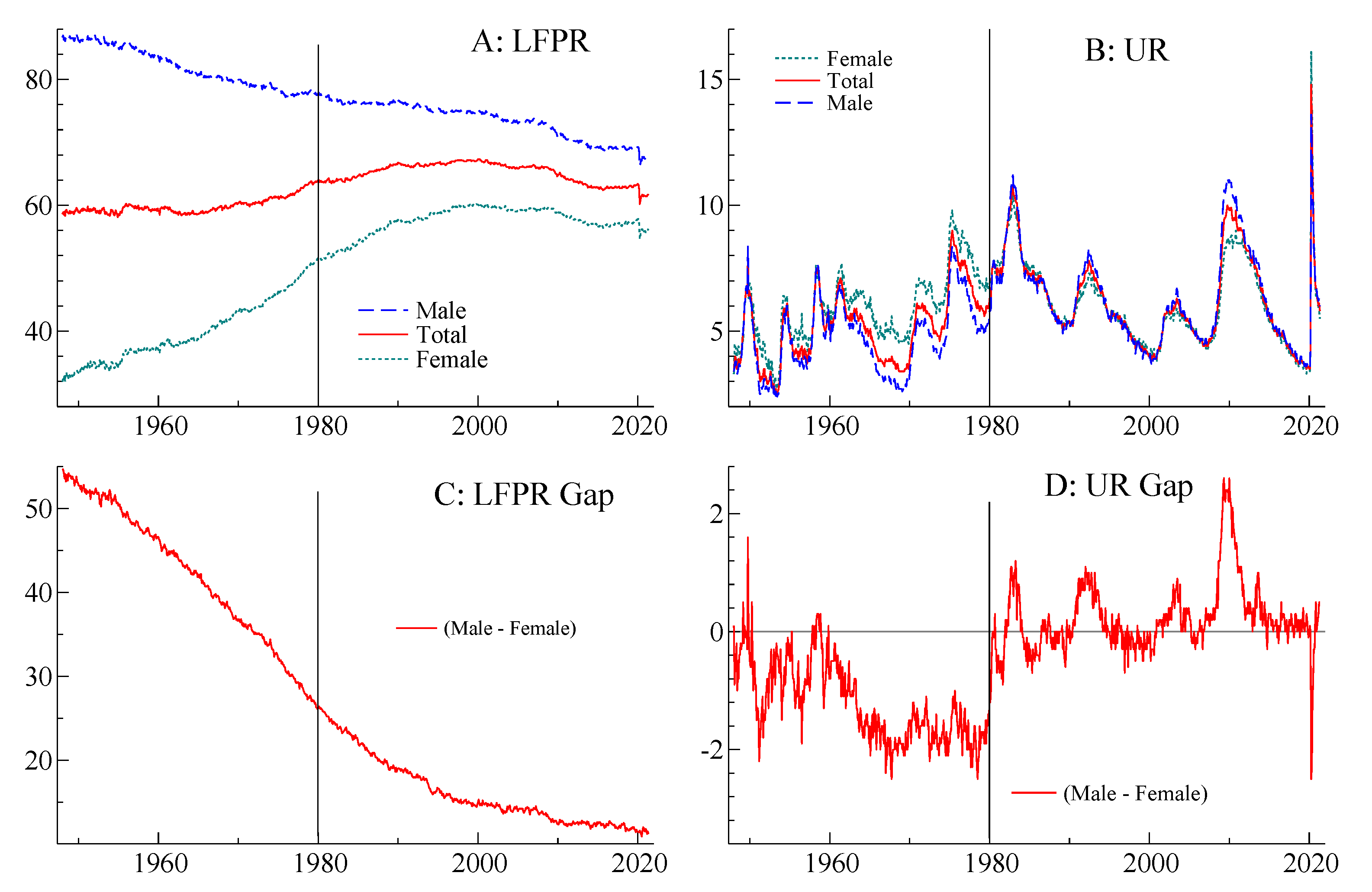
Before extending Emerson’s analysis further, we return to the data and plot them. Panels A and B of Figure 2 plot the total, male, and female labor force participation and unemployment rates. Panel C plots the gap between male and female labor force participation rates and shows how it has fallen considerably over time, with most of the decline occurring in the first three decades of the sample. Panel D shows that, prior to the 1980s, females almost always had higher unemployment rates than men. After 1980, the male and female unemployment rates are much closer together, with men typically having higher unemployment rates than women during recessions—the clear exception being the pandemic-induced recession in 2020.

Figure 2 illustrates several important data features that a model should account for. First, male and female labor force participation rates converge over the sample. Second, the relationship between male and female unemployment rates shifts abruptly around 1980, and that shift appears permanent. This phenomena was analyzed in detail by Albanesi and Şahin (2018) and is explained by the convergence in LFPRs and differences in industry composition. Third, the business cycle has clear and persistent effects, particularly on unemployment but also on labor force participation; see Hobijn and Şahin (2021) for a discussion of the participation cycle.

To address these issues, we make the following changes to the modeling framework. First, we account for the interaction between male and female labor force participation and unemployment rates by modeling them jointly. Second, we focus on the sample 1980–2019, allowing us to formulate a model on a relatively long sample (40 years), during which, the relationships between male and female LFPRs and URs appear to be relatively stable. It also provides a baseline against which to assess how the labor market evolved during the pandemic. We leave modeling the entire post-war sample for future research. Finally, we include 12 unrestricted lags of the NBER recession dummy to better account for persistent effects of recessions over time. This approach is very much in the spirit of White (1990), Hendry and Mizon (1993), and Ericsson et al. (1998), who formalize modeling as a progressive research strategy.

6. A Joint Model of Male and Female LFPRs and URs

This section develops a joint model of male and female labor force participation and unemployment rates. Section 6.1 performs additional bivariate analyses of male and female unemployment rates and of male and female labor force participation rates. Section 6.2 uses these findings to inform restrictions on the cointegrating vectors of a joint four-variable model of the male and female unemployment and labor force participation rates.

6.1. Bivariate Model Analysis

To help us facilitate our interpretation of the joint analysis, we start with bivariate analyses, looking at the relationship between male and female labor force participation rates and the relationship between male and female unemployment rates. In particular, we hypothesize that there are one-to-one long-run relationships between male and female LFPRs and between male and female URs. This framework is motivated by Figure 2, and it contrasts with Emerson (2011), who models the bivariate relationship between LFPR and UR for a given gender.

Table 4. Bivariate system results for 1980–2019.

	LFPR	UR
Trace Statistics:
$H_0:$ r = 0	26.10 * [0.045]	49.95 ** [0.000]
$H_0:$ r ≤ 1	1.71 [0.971]	14.02 * [0.026]
Restricted Cointegrating Vector:
$Male$	1	1
$Female$	−1	−1
Trend	0	−0.0016 $\left(0.0005\right)$
Restricted Adjustment Parameters:
${\alpha }_M$	0	−0.102 $\left(0.018\right)$
${\alpha }_F$	0.011 $\left(0.002\right)$	0
Test of Over-identifying Restrictions:	${\chi }^2\left(3\right)=0.49\left[0.921\right]$	${\chi }^2\left(2\right)=3.01\left[0.222\right]$
Model Specification Tests:
AR 1-7: F(28,856)=	1.32 [0.128]	1.24 [0.182]
ARCH 1-7: F(28,916)=	0.91 [0.601]	1.18 [0.238]
Normality: ${\chi }^2\left(4\right)$=	3.97 [0.410]	3.54 [0.472]
Hetero: F(177,1254)=	1.02 [0.429]	1.20 [0.050]

Notes: Sample is January 1980–December 2019 ($T=480$). See the Notes for Table 2.

presents the results from this analysis. For the labor force participation rates, we find strong evidence of a single cointegrating vector and do not reject the restrictions imposing a one-to-one long-run relationship between male and female LFPRs. Unlike in the sample analyzed in Table 3, Table 4 shows clear evidence that the linear trend is insignificant in the cointegrating vector over the last four decades. Only the female LFPR responds significantly to the LFPR gap, implying that the male LFPR is weakly exogenous for this relation. The estimated adjustment coefficient implies that the female LFPR responds to a one percentage point gap in the LFPR by approximately 0.13 percentage points per year.

For the unemployment rates, the analysis in Table 4 finds two cointegrating relationships, implying that the unemployment rates are stationary after accounting for recessions. However, if we impose a single cointegrating relationship, a one-to-one relation between male and female URs (i.e., a UR gap) is not rejected. The trend is significant in that estimated long-run relationship, suggesting a steady, albeit small, long-run change in the equilibrium UR gap. In this formulation, only the male UR responds significantly to the UR gap, whereas the female UR is weakly exogenous. The adjustment rate is rapid, at approximately 10 percent per month.

6.2. Joint Model Analysis

These bivariate results help to interpret a four-variable joint model of male and female labor force participation and unemployment rates. The long-run relationships in the bivariate systems should hold in the larger four-variable model because cointegrating relationships are invariant to expansions of the information set, where each bivariate system is augmented to include all four variables. Thus, these bivariate results serve as a starting point for interpreting cointegrating relations in the larger system.

The bivariate analyses conducted in Section 4 and Section 6.1 are also restricted versions of the four-variable VAR. If we test for the restrictions implied by the underlying bivariate VARs in each column of Table 4, they are strongly rejected by the data, with p-values of less than 1%. This indicates that there are important interactions between the variables in the joint system that are lost when analyzed as separate bivariate systems in Table 4.

Table 5. Joint system results for 1980–2019.

	Trace Statistics	Max Statistics
$H_0:$ r = 0	109.10 ** [0.000]	48.45 ** [0.000]
$H_0:$ r ≤ 1	60.64 ** [0.000]	32.13 ** [0.007]
$H_0:$ r ≤ 2	29.52 * [0.015]	19.45 * [0.046]
$H_0:$ r ≤ 3	10.06 [0.126]	10.06 [0.126]
Restricted Cointegrating Vectors:
	LFPR Gap	Male UR	Female UR
$LFP{R}_M$	1	0	0
$LFP{R}_F$	−1	0	0
$U{R}_M$	0	1	0
$U{R}_F$	0	0	1
Trend	0	0	0
Restricted Adjustment Parameters:
${\alpha }_{LFP{R}_M}$	0	−0.021 $\left(0.006\right)$	0
${\alpha }_{LFP{R}_F}$	0.014 $\left(0.003\right)$	0	−0.019 $\left(0.008\right)$
${\alpha }_{U{R}_M}$	0	−0.029 $\left(0.006\right)$	0
${\alpha }_{U{R}_F}$	0.012 $\left(0.004\right)$	0.095 $\left(0.023\right)$	−0.136 $\left(0.030\right)$
Test of Over-identifying Restrictions:		${\chi }^2\left(11\right)=$15.45 [0.163]
Model Specification Tests:
AR 1-7:		F(112,1551) = 1.31 * [0.019]
ARCH 1-7:		F(112,1758) = 0.90 [0.755]
Normality:		${\chi }^2\left(8\right)=$ 7.59 [0.475]
Hetero:		F(460,1446) = 1.07 [0.191]

Notes: Sample is January 1980–December 2019 ($T=480$). See the Notes for Table 2.

presents the trace and max statistics and related results for the joint model of male and female LFPRs and URs. These results show consistent evidence of three cointegrating relationships. Identification of these cointegrating relationships draws on the bivariate cointegration results in Section 6.1. After some manipulation, we are able to clearly interpret the cointegrating relationships of the model and how variables in the system respond to them.

The first cointegrating relationship in Table 5 is the gap between the male and female LFPRs, as found in the first bivariate system in Table 4. The trend is insignificant, and only the female LFPR and the female UR respond directly to disequilbrium in this relationship. The estimated speed of adjustment for the female LFPR is faster than in the bivariate analysis, with a monthly adjustment of approximately 17 percent at an annual rate. However, estimating the actual multi-period adjustment is more complicated because the female UR responds to the LFPR gap and the female LFPR responds to the third cointegrating relationship (female UR).

The second and third cointegrating relations correspond to stationary male and female URs, where their stationarity is evident after controlling for NBER recessions and the recessions’ lagged effects; see Table 4. Thus, the second cointegrating relation is the (stationary) male UR itself, to which the male LFPR and UR and the female UR respond. The third cointegrating relation is the (stationary) female UR, to which the female LFPR and the female UR respond.

Table 5 shows dynamic evidence of discouraged worker effects. The male LFPR decreases in response to an increase in the male UR, and the female LFPR decreases in response to an increase in the female UR. However, the net effect of these dynamics is less obvious for females: the female LFPR also increases in response to an increase in the LFPR gap, thereby capturing the trending decline in the LFPR gap, and the female UR responds to all three cointegrating relations.

Jointly, the male LFPR and the male UR are weakly exogenous for cointegrating vectors involving the LFPR gap and the female UR. That is, the male LFPR and the male UR only respond to the male UR in the long-run, but not to the LFPR gap or the female UR. We can test whether the male LFPR and UR are strongly exogenous to the LFPR gap and the female UR (that is, both weakly exogenous and Granger non-causal) by jointly testing the weak exogeneity restrictions and whether the lags of the changes in female LFPR and UR can be excluded from the equations for male LFPR and UR; see Engle et al. (1983) and Ericsson et al. (1998). This hypothesis is strongly rejected: ${\chi }^2\left(48\right)=78.7$, which has a probability of less than 1% under the null hypothesis. This rejection occurs primarily because changes in the male LFPR respond significantly to lagged changes in the female UR.

The joint system of equations appears to be well-specified, with most of the model specification tests failing to reject the null hypothesis of a correctly specified model. However, some autocorrelation remains in the residuals, possibly driven by the male UR equation. The model could be simplified further by testing for and restricting lag structure. However, since we already see evidence of auto-correlated residuals and do not have a clear guide on how to reduce the model, we choose to not simplify the model further.

The robustness of the model can be assessed using the automatic model selection algorithm “Autometrics”. Here, we perform a robustness check by selecting over lag structure and also over possible outliers and step shifts by saturating the model with impulse and step indicators; see Hendry and Krolzig (2005), Doornik (2009), and Hendry and Doornik (2014).4 To protect against spurious results, we choose a “target gauge” of 0.1%, such that, under the null hypothesis, in which none of the indicators matter, we expect on average to include roughly two irrelevant indicators by chance; see Hendry (1999), Castle et al. (2011), and Johansen and Nielsen (2016).5 We do not detect any relevant outliers or step shifts. This provides further evidence that the model is reasonably well-specified in the sample.

7. Forecasting the Labor Market during the Pandemic

Table 5 thus presents a reasonably well-specified model of male and female LFPRs and URs. This model can help to interpret the effects of the COVID-19 pandemic on the labor market by comparing the data over the pandemic with forecasts from our (pre-pandemic) model. To do so, we estimate the model through December 2019 (as in Table 5) and generate multi-step-ahead forecasts through August 2021.

Figure 3 presents outcomes and the model forecasts for several variables: male and female LFPRs and URs, their changes, male and female employment-to-population ratios (EPOPs) (as derived from the male and female LFPRs and URs), and their changes. Figure 3 shows that, for both men and women, the initial recession caused a sharp decline in the LFPRs and the EPOPs, and a spike in the URs. The United States saw a dramatic jump in unemployment rates, unlike the United Kingdom, which had a job furlough program; see Castle et al. (2021). More than a year after the official end of the U.S. recession, the effects on the labor market continue to be pronounced. Unemployment rates have recently fallen to within two standard deviations of the model’s forecasts. However, the LFPRs and EPOPs continue to be well below their pre-pandemic levels. This is especially striking because the forecasts were generated, and were conditional on the NBER 2020 recession dates. This highlights just how different the pandemic recession was, relative to previous recessions.

Next, we examine how the pandemic differentially affected men and women in the labor market by looking at how the forecasted gaps in LPFR, UR, and EPOP compare to the actual outcomes. Figure 4 plots the results from this exercise. The first row in Figure 4 shows the forecast and actual values for the UR gap, the LFPR gap, and the EPOP gap. The second row in Figure 4 presents the one-month changes in those variables and forecasts.

Unlike previous recessions in this sample, the unemployment gap became large and negative (Panel A). By April 2020, the female UR was nearly three percentage points higher than the male UR. During the initial months of the pandemic recession, the female UR increased to unprecedented levels, as service sector industries—which employ a larger share of women—were disproportionately affected. As the pandemic progressed, the LFPR gap first fell and then increased rapidly (Panel B), with the increase driven by women leaving the labor force, in part due to limited child-care options, particularly during the summer of 2020; see Lim and Zabek (2021). Since then, both the LFPR and UR gaps have returned to pre-pandemic levels. This indicates that, while women were more severely affected at the outset of the pandemic relative to previous recessions, their relative participation in the labor market has recovered and is now in line with historical trends. Seasonal patterns also appear to have altered, making the observed data more volatile because seasonal adjustment failed to fully capture that change.

8. Conclusions

This paper jointly models male and female labor force participation rates and unemployment rates. We examine and extend the approach by Emerson (2011) and then focus on the last four decades of data to jointly model and forecast male and female LFPRs and URs to account for the relationships between those variables. There are three long-run relationships, corresponding to the LFPR gap and to stationarity in both male and female unemployment rates. The female LFPR and UR respond to the LFPR gap. In the long run, the male LFPR and UR only respond to the male UR, whereas the female UR responds to both the male and female URs, as well as the LFPR gap.

During the pandemic, both male and female labor force participation rates declined and unemployment rates rose. However, women were much more adversely affected than men at the outset of the pandemic recession and immediately thereafter. Even so, the gap between male and female labor force participation rates has narrowed more recently, and the gap between them now is around its pre-pandemic level.

There are several possible avenues of future research. First, extending the model over the full post-war sample may allow for additional insights on longer-term trends, such as (potentially) a much stronger convergence in the LFPR gap prior to 1980 and a different equilibrium relationship between male and female unemployment rates.6 The full post-war sample may also benefit from an I(2) cointegration analysis, noting that the LFPR gap is itself strongly trending, and not just the male and female LFPRs; see Juselius (2006). Second, different recessions could have different effects on the labor market.7 Furthermore, additional information, such as the number of COVID-19 cases or the stringency index developed by Hale et al. (2021), could help to better capture the pandemic period.8 Finally, the model could be reformulated in terms of the underlying number of employees, the labor force, and the population. This could allow for the model to address other interesting questions that cannot be answered in the model’s current form, e.g., are unemployed women more likely than men to leave the labor force than to remain unemployed? Such modeling could also help to resolve changes in seasonality. This suggests a fruitful research agenda going forward.

References

- Aaronson, Daniel, Jonathan Davis, and Luojia Hu. 2012. Explaining the Decline in the U.S. Labor Force Participation Rate. Chicago Fed Letter No. 296. Chicago: Federal Reserve Bank of Chicago. [Google Scholar]
- Aaronson, Stephanie, Tomaz Cajner, Bruce Fallick, Felix Galbis-Reig, Christopher Smith, and William Wascher. 2014. Labor force participation: Recent developments and future prospects. Brookings Papers on Economic Activity 2014: 197–275. [Google Scholar] [CrossRef] [Green Version]
- Abraham, Katharine G., and Melissa S. Kearney. 2020. Explaining the decline in the US employment-to-population ratio: A review of the evidence. Journal of Economic Literature 58: 585–643. [Google Scholar] [CrossRef]
- Ahn, Hie Joo, and James D. Hamilton. 2021. Measuring labor-force participation and the incidence and duration of unemployment. Review of Economic Dynamics, 1–32, in press. [Google Scholar] [CrossRef]
- Albanesi, Stefania, and Ayşegül Şahin. 2018. The gender unemployment gap. Review of Economic Dynamics 30: 47–67. [Google Scholar] [CrossRef]
- Bernstein, David H., and Bent Nielsen. 2019. Asymptotic theory for cointegration analysis when the cointegration rank is deficient. Econometrics 7: 6. [Google Scholar] [CrossRef] [Green Version]
- Bluedorn, John, Francesca Caselli, Niels-Jakob Hansen, Ippei Shibata, and Marina M. Tavares. 2021. Gender and Employment in the COVID-19 Recession: Evidence on “She-Cessions”. IMF Working Paper WP/21/95. Washington, DC: International Monetary Fund. [Google Scholar]
- Bullard, James. 2014. The rise and fall of labor force participation in the United States. Federal Reserve Bank of St. Louis Review Q1: 1–12. [Google Scholar] [CrossRef] [Green Version]
- Castle, Jennifer L., Jurgen A. Doornik, and David F. Hendry. 2011. Evaluating automatic model selection. Journal of Time Series Econometrics 3: 1–33. [Google Scholar] [CrossRef] [Green Version]
- Castle, Jennifer L., Jurgen A. Doornik, and David F. Hendry. 2021. The value of robust statistical forecasts in the COVID-19 pandemic. National Institute Economic Review 256: 19–43. [Google Scholar] [CrossRef]
- Castle, Jennifer L., Jurgen A. Doornik, David F. Hendry, and Felix Pretis. 2015. Detecting location shifts during model selection by step-indicator saturation. Econometrics 3: 240–64. [Google Scholar] [CrossRef] [Green Version]
- Doornik, Jurgen A. 1996. Testing Vector Autocorrelation and Heteroscedasticity in Dynamic Models. Nuffield College Working Paper. Oxford: Nuffield College. [Google Scholar]
- Doornik, Jurgen A. 2009. Autometrics. In The Methodology and Practice of Econometrics: A Festschrift in Honour of David F. Hendry. Edited by N. Shephard and J. L. Castle. Oxford: Oxford University Press, pp. 88–121. [Google Scholar]
- Doornik, Jurgen A., and Henrik Hansen. 2008. An omnibus test for univariate and multivariate normality. Oxford Bulletin of Economics and Statistics 70: 927–39. [Google Scholar] [CrossRef]
- Doornik, Jurgen A., and David F. Hendry. 2013. Empirical Econometric Modelling Using PcGive 14: Volume I. London: Timberlake Consultants Press. [Google Scholar]
- Emerson, Jamie. 2011. Unemployment and labor force participation in the United States. Economics Letters 111: 203–6. [Google Scholar] [CrossRef]
- Engle, Robert F., David F. Hendry, and Jean-François Richard. 1983. Exogeneity. Econometrica 51: 277–304. [Google Scholar] [CrossRef]
- Ericsson, Neil R. 2017. How biased are U.S. government forecasts of the federal debt? International Journal of Forecasting 33: 543–59. [Google Scholar] [CrossRef] [Green Version]
- Ericsson, Neil R., David F. Hendry, and Grayham E. Mizon. 1998. Exogeneity, cointegration and economic policy analysis. Journal of Business and Economic Statistics 16: 370–87. [Google Scholar]
- Ericsson, Neil R., David F. Hendry, and Kevin M. Prestwich. 1998. The demand for broad money in the United Kingdom, 1878–1993. Scandinavian Journal of Economics 100: 289–324. [Google Scholar] [CrossRef]
- Ericsson, Neil R., David F. Hendry, and Hong-Anh Tran. 1993. Cointegration, seasonality, encompassing, and the demand for money in the United Kingdom. In Nonstationary Time Series Analysis and Cointegration. Edited by C. P. Hargreaves. Oxford: Oxford University Press, Chapter 7. pp. 179–224. [Google Scholar]
- Fieller, Edgar C. 1954. Some problems in interval estimation. Journal of the Royal Statistical Society: Series B (Methodological) 16: 175–85. [Google Scholar] [CrossRef]
- Fujita, Shigeru. 2014. On the Causes of Declines in the Labor Force Participation Rate. Research RAP Special Report. Philadelphia: Federal Reserve Bank of Philadelphia. [Google Scholar]
- Guidotti, Emanuele, and David Ardia. 2020. COVID-19 data hub. Journal of Open Source Software 5: 2376. [Google Scholar] [CrossRef]
- Hale, Thomas, Noam Angrist, Beatriz Kira, Anna Petherick, Toby Phillips, and Samuel Webster. 2021. Variation in Government Responses to COVID-19. Blavatnik School Working Paper BSG-WP-2020/032. Oxford: Blavatnik School of Government. [Google Scholar]
- Hendry, David F. 1999. An econometric analysis of US food expenditure, 1931–1989. In Methodology and Tacit Knowledge: Two Experiments in Econometrics. Edited by J. R. Magnus and M. S. Morgan. Chichester: John Wiley, Chapter 17. pp. 341–61. [Google Scholar]
- Hendry, David F., and Jurgen A. Doornik. 2014. Empirical Model Discovery and Theory Evaluation: Automatic Selection Methods in Econometrics. Cambridge: MIT Press. [Google Scholar]
- Hendry, David F., and Hans-Martin Krolzig. 2005. The properties of automatic Gets modelling. The Economic Journal 115: C32–C61. [Google Scholar] [CrossRef] [Green Version]
- Hendry, David F., and Grayham E. Mizon. 1993. Evaluating dynamic econometric models by encompassing the VAR. In Models, Methods, and Applications of Econometrics: Essays in Honor of A.R. Bergstrom. Edited by P. C. B. Phillips. Cambridge: Blackwell, Chapter 18. pp. 272–300. [Google Scholar]
- Hobijn, Bart, and Ayşegül Şahin. 2021. Maximum Employment and the Participation Cycle. NBER Working Paper No. 29222. Cambridge: National Bureau of Economic Research. [Google Scholar]
- Hoover, Kevin D., and Stephen J. Perez. 1999. Data mining reconsidered: Encompassing and the general-to-specific approach to specification search. The Econometrics Journal 2: 167–91. [Google Scholar] [CrossRef]
- Hornstein, Andreas, Marianna Kudlyak, and Annemarie Schweinert. 2018. The Labor Force Participation Rate Trend and Its Projections. FRBSF Economic Letter 2018-25. San Francisco: Federal Reserve Bank of San Francisco. [Google Scholar]
- Hotchkiss, Julie, and Fernando Rios-Avila. 2013. Identifying factors behind the decline in the U.S. labor force participation rate. Business and Economic Research 3: 257–75. [Google Scholar] [CrossRef] [Green Version]
- Jacobs, Lindsay, and Suphanit Piyapromdee. 2016. Labor Force Transitions at Older Ages: Burnout, Recovery, and Reverse Retirement. Finance and Economics Discussion Series Working Paper No. 2016-053. Washington, DC: Federal Reserve Board of Governors. [Google Scholar]
- Johansen, Søren. 1988. Statistical analysis of cointegration vectors. Journal of Economic Dynamics and Control 12: 231–54. [Google Scholar] [CrossRef]
- Johansen, Søren. 1991. Estimation and hypothesis testing of cointegration vectors in Gaussian vector autoregressive models. Econometrica 59: 1551–80. [Google Scholar] [CrossRef]
- Johansen, Søren, and Bent Nielsen. 2016. Asymptotic theory of outlier detection algorithms for linear time series regression models. Scandinavian Journal of Statistics 43: 321–48. [Google Scholar] [CrossRef] [Green Version]
- Juselius, Katarina. 2006. The Cointegrated VAR Model: Methodology and Applications. Advanced Texts in Econometrics. Oxford: Oxford University Press. [Google Scholar]
- Karabarbounis, Loukas, and Brent Neiman. 2014. The global decline of the labor share. The Quarterly Journal of Economics 129: 61–103. [Google Scholar] [CrossRef] [Green Version]
- Kelejian, Harry H. 1982. An extension of a standard test for heteroskedasticity to a systems framework. Journal of Econometrics 20: 325–33. [Google Scholar] [CrossRef]
- Kleykamp, David, and Jer-Yuh Wan. 2014. Unemployment and participation rates? Revisiting the US data. Applied Economics Letters 21: 1152–55. [Google Scholar] [CrossRef]
- Krueger, Alan B. 2017. Where have all the workers gone? An inquiry into the decline of the U.S. labor force participation rate. Brookings Papers on Economic Activity 2017: 1–87. [Google Scholar] [CrossRef]
- Lim, Katherine, and Michael A. Zabek. 2021. Women’s Labor Force Exits During COVID-19: Differences by Motherhood, Race, and Ethnicity. Finance and Economics Discussion Series Working Paper No. 2021-067. Washington, DC: Federal Reserve Board of Governors. [Google Scholar]
- Lovell, Michael C. 1983. Data mining. The Review of Economics and Statistics 65: 1–12. [Google Scholar] [CrossRef]
- Lunsford, Kurt G. 2021. Recessions and the Trend in the US Unemployment Rate. Economic Commentary No. 2021-01. Cleveland: Federal Reserve Bank of Cleveland. [Google Scholar]
- Murphy, Kevin M., and Robert Topel. 1997. Unemployment and nonemployment. The American Economic Review 87: 295–300. [Google Scholar]
- Perez-Arce, Francisco, Maria J. Prados, and Tarra Kohli. 2018. The Decline in the U.S. Labor Force Participation Rate. Michigan Retirement Research Center WP 2018-385. Ann Arbor: University of Michigan. [Google Scholar]
- Plant, Robert, Manuel S. Santos, and Tarek Sayed. 2017. Computerization, Composition of Employment, and Structure of Wages. Department of Economics Working Paper No. 2017-09. Coral Gables: University of Miami, Department of Economics. [Google Scholar]
- Pretis, Felix, Lea Schneider, Jason E. Smerdon, and David F. Hendry. 2016. Detecting volcanic eruptions in temperature reconstructions by designed break-indicator saturation. Journal of Economic Surveys 30: 403–29. [Google Scholar] [CrossRef]
- Seshadri, Ananth. 2018. A Meta-Analysis of the Decline in the Labor Force Participation Rate. WP 2018-381. Michigan: University of Michigan, Michigan Retirement Research Center. [Google Scholar]
- Staiger, Douglas, James H. Stock, and Mark W. Watson. 1997. How precise are estimates of the natural rate of unemployment? In Reducing Inflation, Volume 30 of National Bureau of Economic Research Studies in Business Cycles. Edited by C. D. Romer and D. H. Romer. Chicago: University of Chicago Press, Chapter 5. pp. 195–246. [Google Scholar]
- Van Zandweghe, Willem. 2012. Interpreting the recent decline in labor force participation. Economic Review 97: 5–34. [Google Scholar]
- White, Halbert. 1990. A consistent model selection procedure based on m-testing. In Modelling Economic Series: Readings in Econometric Methodology. Edited by C. W. J. Granger. Oxford: Clarendon Press, Chapter 16. pp. 369–83. [Google Scholar]
Figure 1.
Total labor force participation rate (LFPR) and unemployment rate (UR). Note: shaded bars are NBER recessions.
Figure 2.
Labor force participation and unemployment rates by gender.
Figure 3.
Forecasts and outcomes of the pandemic labor market by gender. Notes: DX represents the change in X. Shaded bars are NBER recessions. Fan charts represent two standard deviation ex-ante forecast uncertainty.
Figure 4.
Forecasts and outcomes of the pandemic labor market gender gaps. Note: See the Notes for Figure 3.