
Comprehensive Review: Advancements in Rainfall-Runoff Modelling for Flood Mitigation


1
Research Institute of Engineering and Technology, Hanyang University, Ansan 15588, Korea
2
Department of Civil Engineering & Technology, Qurtuba University of Science and Information Technology, Dera Ismail Khan 29050, Pakistan
3
Department of Agricultural Engineering, University of Engineering & Technology, Peshawar 25000, Pakistan
4
Laboratory of Water & Environment, Faculty of Nature and Life Sciences, Hassiba Benbouali University of Chlef, Chlef 02180, Algeria
5
Department of Civil and Environmental Engineering, Hanyang University, Ansan 15588, Korea
*
Author to whom correspondence should be addressed.
Climate 2022, 10(10), 147; https://doi.org/10.3390/cli10100147
Submission received: 2 September 2022
/
Revised: 29 September 2022
/
Accepted: 8 October 2022
/
Published: 10 October 2022
(This article belongs to the Special Issue Natural Disasters and Extreme Hazards under Changing Climate)
Abstract
:Runoff plays an essential part in the hydrological cycle, as it regulates the quantity of water which flows into streams and returns surplus water into the oceans. Runoff modelling may assist in understanding, controlling, and monitoring the quality and amount of water resources. The aim of this article is to discuss various categories of rainfall–runoff models, recent developments, and challenges of rainfall–runoff models in flood prediction in the modern era. Rainfall–runoff models are classified into conceptual, empirical, and physical process-based models depending upon the framework and spatial processing of their algorithms. Well-known runoff models which belong to these categories include the Soil Conservation Service Curve Number (SCS-CN) model, Storm Water Management model (SWMM), Hydrologiska Byråns Vattenbalansavdelning (HBV) model, Soil and Water Assessment Tool (SWAT) model, and the Variable Infiltration Capacity (VIC) model, etc. In addition, the data-driven models such as Adaptive Neuro Fuzzy Inference System (ANFIS), Artificial Neural Network (ANN), Deep Neural Network (DNN), and Support Vector Machine (SVM) have proven to be better performance solutions in runoff modelling and flood prediction in recent decades. The data-driven models detect the best relationship based on the input data series and the output in order to model the runoff process. Finally, the strengths and downsides of the outlined models in terms of understanding variation in runoff modelling and flood prediction were discussed. The findings of this comprehensive study suggested that hybrid models for runoff modeling and flood prediction should be developed by combining the strengths of traditional models and machine learning methods. This article suggests future research initiatives that could help with filling existing gaps in rainfall–runoff research and will also assist hydrological scientists in selecting appropriate rainfall–runoff models for flood prediction and mitigation based on their benefits and drawbacks.
1. Introduction
Hydrology is concerned with the earth’s water, its occurrence, circulation, and distribution, as well as its chemical and physical properties and interaction with the environment, particularly its relationship with living organisms [1]. Hydrology is also concerned with the interaction of water with the environment at each stage of the hydrologic cycle. The hydrological cycle contains several interrelated components; for example, streamflow is connected with precipitation [2]. Surface runoff occurs when rainwater does not infiltrate into the soil due to the saturated condition of the soil, and the water flows over the land surface into surface waterways such as rivers, streams, reservoirs, and lakes [3]. Surface runoff is a key component of water resource monitoring as well as resolving water quality and quantity issues like flood predictions and ecological and biological connections in the aquatic environment [4]. Runoff is also a major contributor to contaminant transport because surplus nutrients and pesticides from agricultural lands are transported into rivers by runoff events [5]. Information about pollution caused by runoff is necessary for water managers to take preventive measures for safe water resources. Variations in hydrologic systems have been observed due to a rapid increase in urbanization including deforestation, land cover change, industrialization, irrigation, etc. [6]. Climate change and soil heterogeneity also have a serious influence on the surface flows of many rivers globally [7]. Runoff modelling is essential for better understanding the impact of all the changes on hydrological phenomena [8].
Runoff models depict what happens in water systems as a result of changes in impervious areas, vegetation, and weather events. Devia et al. [9] describes a runoff model as a series of equations that help in the calculation of the quantity of rainfall that converts into runoff as a function of several parameters used to characterize the watershed. Modelling runoff is an extremely difficult process due to the convoluted interaction of various interconnected elements [2,10]. Runoff modelling is utilized to better understand watershed productivity and reactions as well as to predict water availability, track changes over time, and forecast extreme disasters (floods and droughts) [11]. For example, the hydrological model Hydrological Simulation Program-Fortran (HSPF) predicts nutrients, sediment loads, toxic chemicals, pesticides, and other water quality concentrations from the runoff as part of its capabilities [12]. There are many distinct types of rainfall–runoff models available across the world; however, none of them fit into a single category because they were built for diverse objectives [13]. According to Moradkhani and Sorooshian [14], the optimal model is one that produces results near to reality while using the fewest parameters and least model complexity. The most important inputs required for rainfall–runoff models to simulate runoff include rainfall, temperature, watershed topography, vegetation, hydrogeology, and other physical parameters [9].
Hydrological models are classified into empirical models, conceptual models, physical process-based models, and data-driven models [2,9,15]. Traditional empirical models such as the Rational Method, Horton’s Model, Curve Number Model, the Agricultural Catchment Research Unit (ACRU), and the Green Ampt Infiltration Model have been utilized in order to simulate runoff [16,17,18,19,20]. The main drawbacks of these models are that they rely on field observations that are not always accessible. The physical process-based models follow the principles of physical processes in modelling runoff, and these models represent catchment behavior in terms of differential equations in both space and time [9]. They work by describing mass and momentum balance for each sub-catchment and employing mutual boundary conditions to connect sub-systems [21]. The physical process-based models do not need large meteorological and hydrological datasets for calibration. On one hand, these models need the assessment of a large number of physical characteristics that determine watershed morphology [9,15]. The most widely used physical process-based models to simulate hydrological processes include the Systeme Hydrologique European (SHE) model, Soil and Water Assessment Tool (SWAT), Institute of Hydrology Distributed Model (IHDM), etc. [21,22]. According to Chiew et al. [23], physical process-based models include a lot of parameters and have data limitations. Conceptual models define a catchment as a collection of connected storage units, and the flow movement between them is specified by mathematical functions. They include simple time series models, the Sacramento Model, the 17-Parameter Stanford Model, the Hydrologiska Byråns Vattenbalansavdelning (HBV) model, the GR4J Model, etc. [24,25,26]. A major restriction of these models is that their parameters cannot be directly assessed from the catchment, and thus they must be calibrated [27]. These downsides of empirical, physical-based, and conceptual models urge the use of advanced data-driven models, such as machine learning (ML) and deep learning (DL).
In recent decades, data-driven models have gained considerable attention from hydrologists in rainfall–runoff modelling. The most commonly used data-driven models in rainfall–runoff modelling include machine learning, time series models, probabilistic models, regression models, and hybridized models [28]. Safari et al. [29] used the Multivariate Adaptive Regression Splines (MARS), Radial Basic Function (RBF), and Reproducing Kernel Hilbert Space (RRKHS) methods to simulate runoff in Turkey. Mohammadi et al. [30] demonstrated that ML models can accurately simulate streamflow series in four rivers in the United States and Canada. The main advantage of data-driven models is that they statistically formulate rainfall–runoff nonlinearity solely based on historical data and do not require any knowledge of fundamental physical processes [15].
Flooding is among the most destructive natural calamities resulting in fatalities and can endanger multiple sectors [31]. The three main types of flooding are river floods, coastal floods, and flash floods. A flash flood is the result of runoff from excessive rainfall which raises the water level in a stream or normally dry channel over a short period (mostly less than 6 h). Among the three types of flooding, flash floods accounted for the highest flood-induced deaths globally [32]. Researchers and decision-makers are in agreement that flash flood risk management is vital for reducing different losses [33]. Understanding rainfall–runoff modelling plays a crucial role in identifying the regions of high flood risk. Though hydrologic and hydraulic modelling is much appreciated globally, the outputs from these models need more attention in order to realize true watershed flow dynamics. Hence, selecting the right category of models or knowledge-based integration of different models could be an effective tool in flood risk assessment [31,32,33,34,35].
The main objectives of this review are: (1) to give an overview of different rainfall–runoff modelling approaches and their recent applications, (2) to describe the performance of rainfall–runoff models for flood prediction.
2. Overview of Rainfall–Runoff Modelling Approaches
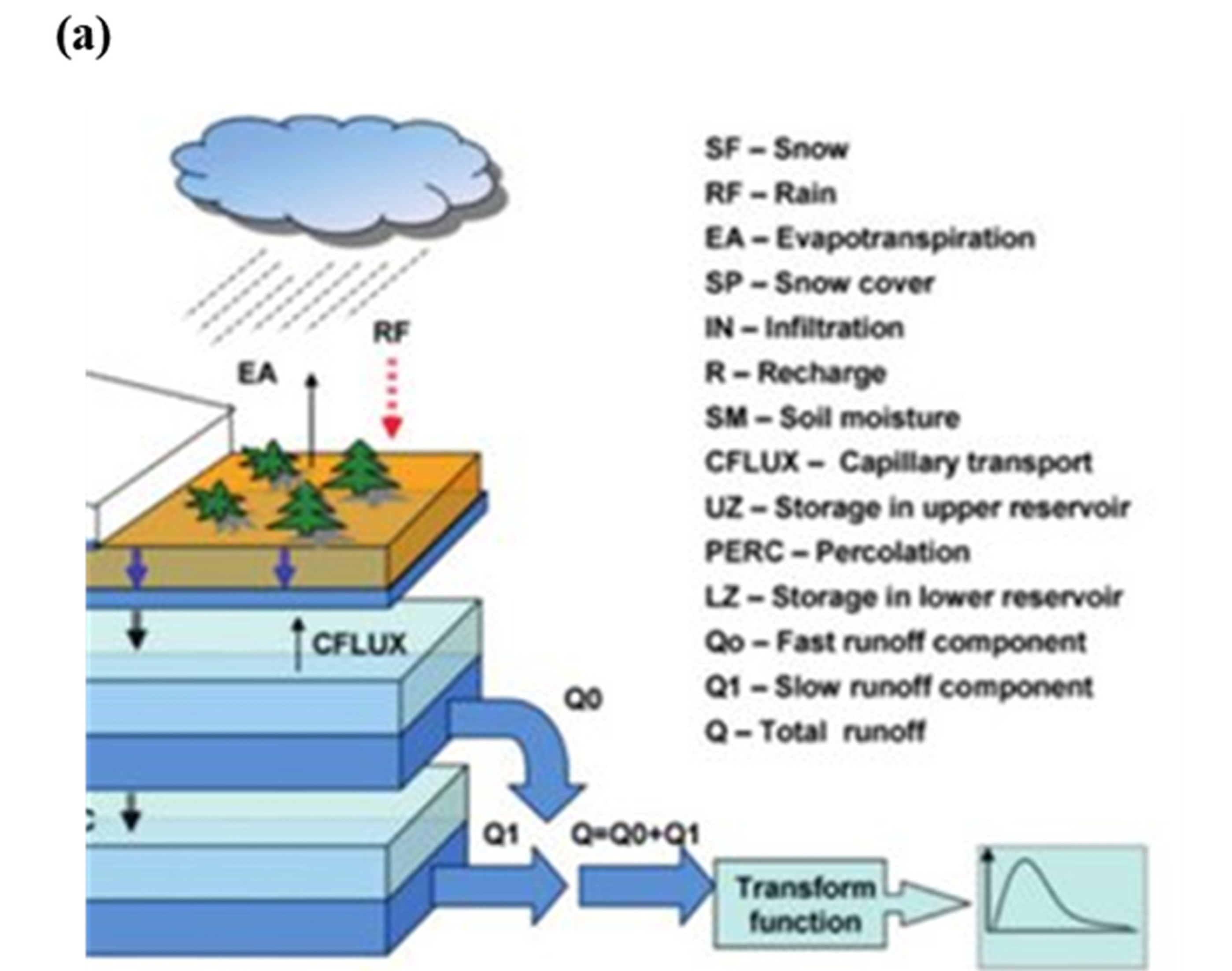
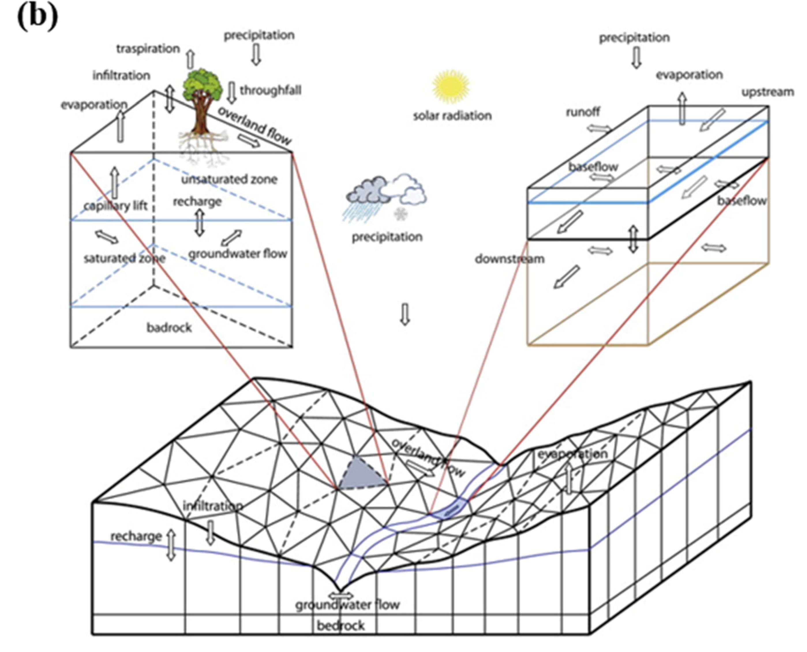
A variety of rainfall–runoff models have been developed and deployed for the management of water resources. Rainfall–runoff models are broadly classified into conceptual models, physical process-based models, and empirical models [36]. A schematic diagram of conceptual models, physical process-based models, and empirical models is shown in Figure 1.
This classification is based on model input and its parameters as well as the extent to which physical concepts are implemented in the models. Each model, with its own set of features, has therefore been implemented with varying degrees of success, from small basins to large catchments, encompassing both ungauged and gauged catchments [37]. Further, each model has various downsides such as large data requirements, complexity in parameter estimation, and less user-friendliness. Detailed characteristics of conceptual models, physical models, and empirical models are provided in Table 1.
2.1. Conceptual Models
Dooge [51] defines conceptual models as “models formed on the basis of a simple arrangement of a relatively limited number of components, each of which is itself a simple representation of a physical connection”. Conceptual models depict the water balance equation with the transformation of rainfall to runoff, evapotranspiration, and subsurface water as expressed in Equation (1) [52].
where, , , , , and are precipitation, evapotranspiration, surface runoff, groundwater, and change in storage, respectively.
Conceptual models employ semi-empirical equations, and model parameters are determined not only from field measurements but also through calibration [53]. The calibration of conceptual models requires a large amount of hydro-meteorological data. Lumped hydrological models fall under the category of conceptual models. A watershed is treated as a single homogeneous unit in a lumped conceptual rainfall–runoff model, which averages total rainfall, its distribution over space, soil properties, overland flow conditions, etc. In some situations, lumped rainfall–runoff models produce good results after calibration with historical input–output data of watershed [54]. Numerous lumped rainfall–runoff models have been developed and implemented, such as HBV, GR2M, ABCD, TANK, etc. [55,56,57,58]. Jehanzaib et al. [40] successfully employed a GR2M and ABCD model to reconstruct streamflow series in South Korean territory with good model performance. The primary purpose of lumped conceptual models is to estimate runoff; nevertheless, they are often built to simulate actual evapotranspiration in order to account for soil water balance, and they have no direct interest in predicting surface energy fluxes [59]. The parameters of lumped rainfall–runoff models are normally tuned such that the simulated runoff matches the observed runoff as much as possible. To assure conformity between model simulations of system behavior and observations, several model calibration procedures have been devised and applied [60]. Lumped rainfall–runoff models are simple, require less input data, and their calibration cost is inexpensive compared to distributed models. These models are quite easy to use and are important tools for hydrologic analysis. Vansteenkiste et al. [61] conducted a comparative study of five hydrological models in a medium-sized catchment in Belgium in order to check the accuracy of lumped and distributed models. They concluded that the lumped hydrological models took less time for calibration and produced higher model performance as compared to distributed models. Reed et al. [62] also compared the performance of 12 distributed models with a lumped model and reported that the performance of lumped models remained on the higher side as compared to distributed models, but some distributed models perform better than a trained lumped model. In conclusion, due to their simplicity and applicability, lumped models are still highly significant tools in hydrological modelling, particularly for estimating runoff in ungauged catchments.
2.2. Physical Process-Based Models
Physical process-based models are idealized mathematical descriptions of real phenomena. These are also known as mechanistic models, since they involve physical process concepts. Distributed models lie in the category of physical process-based models. In a distributed model, all the hydrological phenomena, including runoff generation, snow buildup and melt, recharging to groundwater, evapotranspiration, soil moisture dynamics, and routing in lakes and rivers, are interrelated [63]. The parameters of distributed models reflect the spatial variation of characteristics across the watershed while also distinguishing between changes in the hydrologic processes that occur throughout the watershed. Every small element of the watershed is modeled separately to account for hydrological connection with the adjacent element [64].
The distributed models may be utilized to estimate the influence of land use and land cover changes on runoff and the availability of water [65]. These models are especially important for watersheds with diverse climate and land surface conditions. In 1979, a semi-distributed TOPMODEL was developed to describe the runoff generation process by incorporating both infiltration and saturation excess according to a topographical index derived from the digital elevation model (DEM) [66]. The TOPMODEL does not consider the spatial variability of precipitation. After the development of TOPMODEL, three fully distributed hydrological models, namely the System Hydrologic European (SHE), MIKE-SHE, and the Soil and Water Assessment Tool (SWAT), were developed to take into account increasingly complicated hydrological processes [22,67]. The United States Environmental Protection Agency (EPA) developed the Storm Water Management Model (SWMM) [68]. SWMM is a dynamic rainfall–runoff model that can be used to simulate the quantity and quality of runoff from metropolitan areas [46,47,69,70]. A well-known rainfall–runoff model, the Hydrologic Engineering Center-Hydrologic Modeling System (HEC-HMS) is widely used in climate impact assessment studies [43,71]. Similarly, the Hydrologic Research Center Distributed Hydrologic Model (HRCDHM), Waterloo Flood Forecasting Model (WATFLOOD), Institute of Hydrology Distributed Model (IHDM), etc., have been used for runoff simulation and flood modelling [44,72,73].
Several researchers demonstrated that no single model consistently performs well, but rather that individual model performances fluctuate depending on the setting [62,74,75]. The selection of a distributed model depends on the study objectives, application, and data availability. Despite the complexity of distributed hydrological models, they are extremely useful for studying changes in hydrological processes induced by man-made activities including urbanization, industrialization, deforestation, water extraction, etc. Im et al. [45] used a calibrated SHE model to investigate the impact of land-use changes on the hydrological response and predicted streamflow well within the Gyeongancheon watershed in South Korea. Zhang et al. [76] also found the SHE model very useful to understand the rainfall–runoff mechanism in northwestern China. Yin et al. [77] demonstrated that the MIKE FLOOD model and the integrated SWMM and Cellular Automata Dual-Drainage Simulation (CADDIES) 2D model performed similarly for runoff simulation. Mobilia et al. [78] compared the performance of three hydrological models: the Nash Cascade Model, SWMM, and the HYDRUS-1D model. The findings suggested that the SWMM model and HYDRUS model perform well with an average Nash–Sutcliffe efficiency (NSE) 0.65, while the Nash Cascade Model was found to be superior with NSE 0.73. The availability of extensive databases is one reason why distributed parameter models have not been widely used. Future advancements in data collection, such as the use of geographical information systems (GIS), will likely lead to greater usage of distributed hydrological models.
2.3. Empirical Models
Empirical models are observation-based models which rely solely on current data without taking into account the characteristics and processes of the hydrological system, and these models are also known as data-driven models [53]. They use mathematical equations generated from simultaneous input and output time series rather than physical processes of the watershed. Majority of empirical models are black-box models, which means that very little or no information about the internal process that generates runoff results is known [2,79]. In empirical models, the governing equation for calculating runoff is a function of inputs as expressed in Equation (2) [80]:
where X and Y are precipitation and historic runoff.
Unit hydrograph (UH) and Soil Conservation Service Curve Number (SCS-CN) are simple empirical models. Statistical-based empirical models employ regression and correlation methods to determine the functional connection between inputs and target variables. Machine learning approaches employ data-driven artificial neural networks (ANN) that self-train to understand the relationship between rainfall and runoff. The empirical models are best employed when no extra outputs are required; for instance, this type of model cannot determine the distribution of runoff across upstream and downstream areas. Empirical models perform good modelling results in ungauged watersheds owing to a lack of particular knowledge about the watershed [81]. Empirical models can produce reliable simulations in a variety of conditions, including longer time steps and reconstructing historical runoff values, because they need few parameters [8]. Empirical models are selected for a variety of reasons, including ease of implementation, quicker calculation speeds, and cost efficiency [49]. Empirical models are data-driven, so input is the main source of uncertainty; any misinterpretation of input data has substantial consequences on the predicted output. One disadvantage of empirical models is that they may yield results that differ from what accepted theoretical analysis would recommend [2]. The most prominent limitation of empirical models is that their parameters cannot be directly determined from the watershed, hence they need to be calibrated [27].
3. Machine Learning Methods for Rainfall–Runoff Modelling
It has been scientifically proven that the forecast of the river system and its runoff pattern is particularly challenging owing to natural changes and physical processes associated with the river system. In hydrological modelling, the desire to increase the accuracy and reliability of hydrological variable predictions has received a great deal of attention [82]. Owing to model instability and runoff behavior, such as extreme episodes in historical records, a substantial number of models are unable to provide reliable forecasts [83]. Therefore, researchers have focused on developing more robust and sophisticated machine learning (ML) methods for runoff modelling and flood prediction in recent years [84]. In ML models, the association between hydrological cycle variables and runoff is examined directly without regard for the actual processes involved [85]. However, such ML (black-box) approaches are good enough at modelling runoff [86,87]. The most widely used ML approaches in hydrologic research are K-nearest neighbor (K-NN), decision tree (DT), fuzzy rule-based systems (FRBS), ANN, deep neural networks (DNN), adaptive neuro-fuzzy inference system (ANFIS), and support vector machine (SVM), etc. Numerous researchers have utilized these ML models for rainfall–runoff analysis. The pros and cons of these ML models are listed in Table 2.
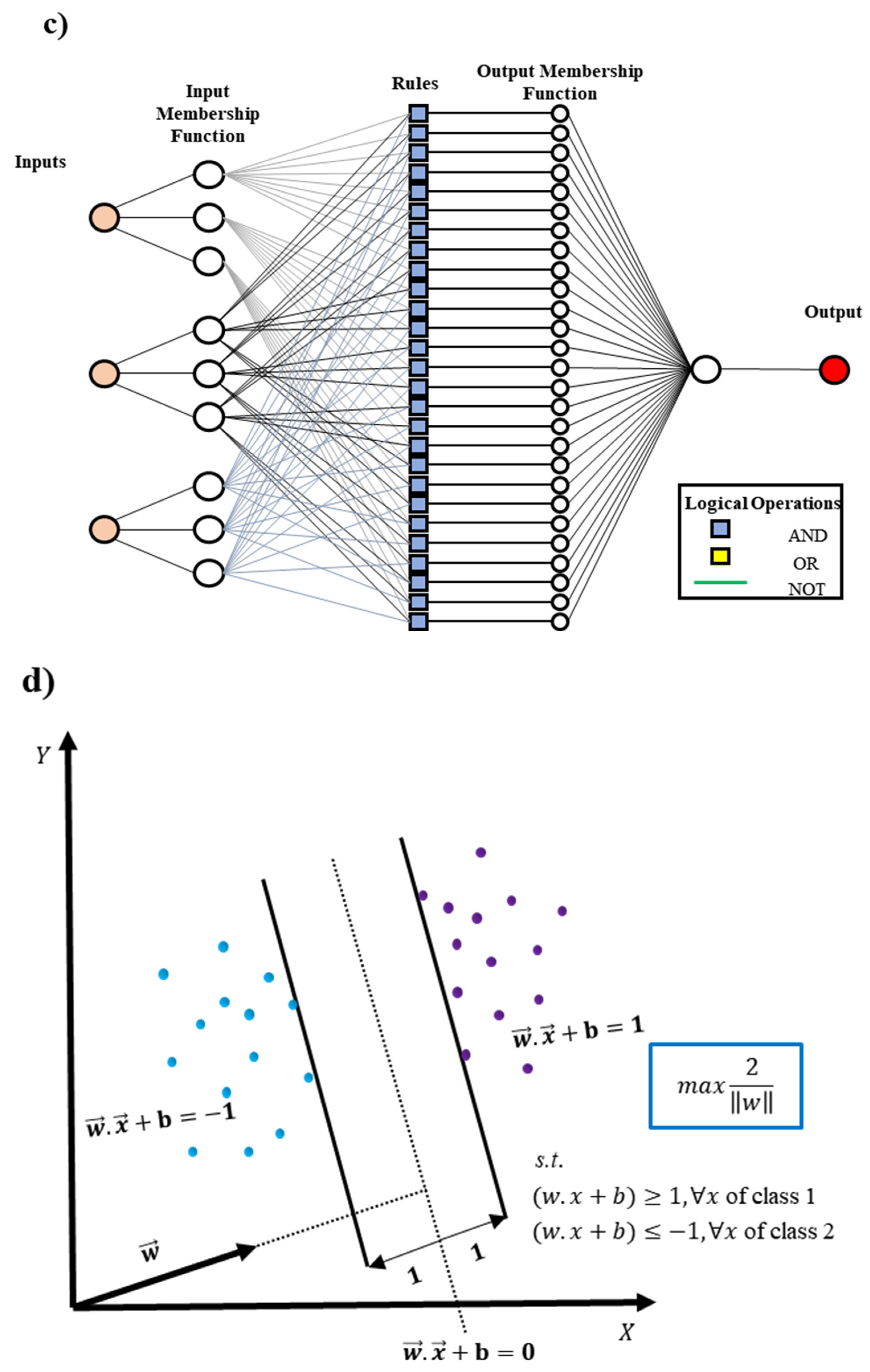
The schematic diagram of most commonly used ML models such as ANN, DNN, ANFIS, and SVM is presented in Figure 2.
3.1. Artificial Neural Network (ANN)
The ANN is a highly distributed parallel information processing model with certain performance attributes analogous to the human brain [105]. The structure of ANN is composed of three layers: (i) input layer, (ii) hidden layer, and (iii) output layer. The ANN networks are trained through several learning algorithms such as feed-forward back propagation (FFBP), radial basis function (RBF), and Generalized regression neural network (GRNN). In engineering applications, the FFBP is the most extensively adopted ANN for non-linear generic guesstimates [106]. ANN models have been utilized by many previous studies [99,100,101,107]. Wu et al. [99] employed a multi-layer neural network for runoff prediction (four steps ahead or 1 hour ahead) and concluded that as the number of prediction steps rises, the model’s accuracy falls. Therefore, the findings of predicting one step ahead are more accurate than the outcomes of two-step-ahead prediction. Kişi [101] compared four different ANN training algorithms (backpropagation, Levenberg Marquardt, cascade correlation, and conjugate gradient) in predicting short-term daily runoff and concluded that the performance of the LM algorithm is better in terms of computation time and accuracy than the other three algorithms. Jain and Kumar [107] proposed a hybrid ANN model by incorporating a general modelling framework and reported that the hybrid ANN model performs better than the traditional ANN. Similarly, Mutlu et al. [100] compared the performance of two different types of ANN models including the MLP and RBF in order to predict runoff at four distinct stations and confirmed the superiority of the MLP model over the RBF model in predicting surface runoff. The deep neural networks (DNN), convolutional neural network (CNN), long short-term memory (LSTM), and recurrent neural network (RNN) are the advanced forms of ANN, and they are also becoming common of late in rainfall–runoff modelling [96,97,98,108]. Contrarily, the ANNs and DNNs have noticeable limitations including over-fitting issues, local minima, learning rate processes, computation time, computation cost and simple manual interventions such as training. However, experts can overcome all the aforementioned difficulties and achieve high accuracy in the runoff modelling process by adjusting specific neural network settings.
3.2. Adaptive Neuro-Fuzzy Inference System (ANFIS)
The ANFIS is a prominent soft computing approach capable of estimating any real continuous function is a compact set to any level of precision [109]. The ANFIS model combines the strength of both fuzzy logic with neural networks to model uncertain situations correctly. The ANFIS is a commonly used model for runoff simulation [102,103,110,111]. El-Shafie et al. [110] utilized the ANFIS model for monthly runoff forecasting and compared its performance with ANN. The findings suggested that the ANFIS model was capable of forecasting inflow with high accuracy, especially in severe inflow conditions, as compared to ANN. Özger [111] employed the Takagi Sugeno Fuzzy Inference System (TS) to simulate runoff series. The TS rule was based on a series of linear functions for predicting runoff. The TS relationship function took into account all of the uncertainty and complexity of the suggested model, and the correlation between the observation and prediction values was found to be satisfactory. Pramanik and Panda [103] compared the performance of two ML methods such as ANN and ANFIS that trained on upstream flow data in order to predict downstream flow. The finding suggested that the neural network with a conjugate gradient algorithm performs better than the LM and gradient descent algorithms, while the ANFIS estimated outflow better than ANN. Sanikhani and Kisi [102] developed two distinct ANFIS models (ANFIS with sub-clusters [ANFISSC] and ANFIS with separated grids [ANFISGP]) for streamflow simulation at a monthly time scale. Both proposed models were utilized to predict runoff 1 month ahead, but the performance of the ANFISSC model was slightly superior to ANFISGP in predicting river flow. The widespread implementation of ANFIS for rainfall–runoff modelling is due to the fact that the fuzzy inference system can handle missing and convoluted data that characterize the runoff. Generally, it is difficult to characterize runoff precisely; an estimation approach (fuzzy set) was suggested in ANFIS to produce reasonable results in runoff modelling. Several researchers highlighted the advantages of ANFIS, which enabled them to obtain high-accuracy results for runoff modelling at various time scales.
3.3. Support Vector Machine (SVM)
The basic principle of SVM is to translate the original data from the input space to a higher dimension space, so the classification problem becomes easy in that feature space. In SVM, support vectors are used as selection criteria, and these support vectors produce the optimal data categorization boundaries [112]. Many studies have recently investigated the capability of SVM in the runoff modelling procedure. Bray and Han [113] highlighted the use of SVM to determine the suitable model structure and associated parameters to simulate runoff in the Bird Creek watershed. They created a flowchart for model identification in order to investigate the interaction between various model structures such as kernels (linear, sigmoidal, radial, and polynomial), scaling factors, and model parameters (cost and epsilon), and input vector composition. Li and Cheng [93] utilized three ML approaches, namely ANN, SVM, and an extreme learning machine (ELM), for runoff prediction for two reservoirs in China. The findings suggested that all the ML methods simulated streamflow quite efficiently, while the SVM simulated runoff with a high correlation value (0.91) in the validation stage. Similarly, He et al. [114] compared the performance of three ML techniques, namely ANN, ANFIS, and SVM, for modelling runoff in a semi-arid climate. Various input combinations were tested, and the most appropriate input variables were selected for streamflow modelling. The results showed that the performance of the SVM model was superior as compared to the ANFIS and ANN models. These ML techniques also have capabilities to decrease the generalized error of the model in addition to the mean square error (MSE) of the training dataset. Most of the researchers reported that the radial-based kernel function of SVM is most suitable for runoff modelling because radial-based kernel has fewer adjustment parameters as compared to polynomial and sigmoidal kernels. Using a radial kernel, the SVM model captures the situation wherein the relationship between inputs and outputs is non-linear. The SVM model is more suitable for long-term streamflow simulation in comparison to short-term streamflow simulation.
4. Flood Risk Assessment
Increasing greenhouse gas concentrations in the atmosphere are projected to result in an increase in global average temperature as well as changes to precipitation and evapotranspiration rates. These climatological shifts may result in extreme natural disasters such as floods and droughts [115]. Rainfall–runoff models were employed by many researchers to examine water resource management on a regional scale, as well as to determine the effects of climate change on hydrology. Sood et al. [116] implemented SWAT model using climatic data to investigate the impact of climate change on floods in the Volta river basin, West Africa, and found a 40% decrease in river flow. Mostafazadeh et al. [117] reported that the HEC-HMS model was particularly useful for modelling various flood control scenarios and estimating varying percentage of peak flood reduction. Peredo et al. [118] adapted a semi-distributed hydrological model (GRSD) with modifications to simulate flood events occurring under different conditions in the Mediterranean region and concluded that the modified model performed better than the original model. Van den Honert and McAneney [119] reported the failure of hydrological models in the prediction of floods that occurred in Queensland, Australia in 2010. Similarly, numerical prediction models were regarded as a step forward in deterministic computations, but they were found to be unreliable due to systematic problems. [120].
Over the previous two decades, the continual progress in machine learning methods has proved their applicability for flood forecasting with an acceptable rate of outperforming traditional approaches. Panda, et al. [121] compared the performance of ANN with a physical process-based MIKE 11 model for water level prediction and concluded that the performance of ANN was superior. Modaresi et al. [122] evaluated the prediction ability of various ML models such as K-nearest neighbor (KNN), ANN, least-square support vector regression (LS-SVR), and generalized regression neural network (GRNN), for flood detection in Karkheh Dam, Iran. They concluded that ANN performs best. Sankaranarayanan et al. [123] used SVM, KNN, and Nave Bayes for flood forecasting in Bihar and Oris-sa and compared their performance with DNNs. The results showed that DNN had a higher level of accuracy. Modern studies [124,125,126] recommended that the development of hybrid models by combining the strengths of conceptual models and ML models will be beneficial for effective flood risk assessment.
5. Conclusions
A wide range of rainfall–runoff models with multiple applications ranging from small watersheds to global-scale models are available. Some models are comprehensive and rely on physical processes of the hydrological cycle and consider space and time during analysis. These models are used to model gauged and ungauged watersheds, which assist in water management, sedimentation and erosion management, water quality assessment, nutrients circulation, climate change impact assessment, etc. Each model has its own set of drawbacks such as a large number of data requirements, limited user accessibility, lack of explanations about its capabilities, etc. Models must incorporate major developments in remote sensing technology, risk assessments, and other areas in order to address these shortcomings. New conceptual and physical process-based models should incorporate advanced statistical techniques for simulating in gauged and ungauged watersheds.
Meanwhile, empirical models, particularly advanced ML models, have proven to be valuable tools for runoff modelling and flood prediction in various regions with high accuracy. The main advantage of ML models is their limited data requirement and easy applicability. They utilize numerous non-linear mathematical theories in order to build relationships between input and output data. Determining efficient input parameters is critical to achieving optimal ML model performance. Furthermore, various studies have identified that ML models should be utilized with caution due to their non-linear character, which can lead to over-fitting issues. It is recommended that future potential researchers utilize the latest optimization algorithms while training the ML models in order to reduce these limitations. ML models have great potential to simulate runoff accurately if these limitations are overcome. Meanwhile, a few modern studies have developed hybrid models by integrating conceptual and ML models for flood prediction and have recommended that hybrid models are highly suitable for runoff modelling and flood prediction. Future researchers are encouraged to develop new hybrid-based models that combine physical process-based models with machine learning models for streamflow simulation investigations and flood risk predictions, as effective predictions lead to successful mitigation measures.
Author Contributions
Conceptualization, M.J.; methodology, M.J.; validation, M.J., M.A. (Mohammed Achite) and T.-W.K.; formal analysis, M.J.; investigation, M.J. and M.A. (Muhammad Ajmal); resources, M.A. (Mohammed Achite) and T.-W.K.; data curation, M.J. and M.A. (Muhammad Ajmal); writing—original draft preparation, M.J.; writing—review and editing, M.A. (Muhammad Ajmal), M.A. (Mohammed Achite) and T.-W.K.; visualization, M.J. and M.A. (Muhammad Ajmal); supervision, T.-W.K.; funding acquisition, M.J. and T.-W.K. All authors have read and agreed to the published version of the manuscript.
Funding
This research was supported by the Lower-Level and Core Disaster Safety Technology Development Program funded by the Ministry of Interior and Safety (Grant No. 2020-MOIS33-006).
Institutional Review Board Statement
Not applicable.
Informed Consent Statement
Informed consent was obtained from all subjects involved in the study.
Data Availability Statement
Some or all data, models, or code that support the findings of this study are available from the corresponding author upon reasonable request.
Acknowledgments
Thanks to peer reviewers who improved this manuscript. We thank the Lower-Level and Core Disaster Safety Technology Development Program funded by the Ministry of Interior and Safety (Grant No. 2020-MOIS33-006).
Conflicts of Interest
The authors declare no conflict of interest.
References
- Linsley, R.K., Jr.; Kohler, M.A.; Paulhus, J.L. Hydrology for Engineers; McGraw-Hill: New York, NY, USA, 1975. [Google Scholar]
- Beven, K.J. Rainfall-Runoff Modelling: The Primer; John Wiley & Sons: Hoboken, NJ, USA, 2011. [Google Scholar]
- Yang, W.-Y.; Li, D.; Sun, T.; Ni, G.-H. Saturation-excess and infiltration-excess runoff on green roofs. Ecol. Eng. 2015, 74, 327–336. [Google Scholar] [CrossRef]
- Kokkonen, T.; Koivusalo, H.; Karvonen, T. A semi-distributed approach to rainfall-runoff modelling—A case study in a snow affected catchment. Environ. Model. Softw. 2001, 16, 481–493. [Google Scholar] [CrossRef]
- Howarth, R.W.; Anderson, D.; Cloern, J.E.; Elfring, C.; Hopkinson, C.S.; Lapointe, B.; Malone, T.; Marcus, N.; McGlathery, K.; Sharpley, A.N. Nutrient pollution of coastal rivers, bays, and seas. Issues Ecol. 2000, 7, 1–16. [Google Scholar]
- Jehanzaib, M.; Shah, S.A.; Yoo, J.; Kim, T.-W. Investigating the impacts of climate change and human activities on hydrological drought using non-stationary approaches. J. Hydrol. 2020, 588, 125052. [Google Scholar] [CrossRef]
- Salvadore, E.; Bronders, J.; Batelaan, O. Hydrological modelling of urbanized catchments: A review and future directions. J. Hydrol. 2015, 529, 62–81. [Google Scholar] [CrossRef]
- Xu, C. Hydrologic Models; Uppsala University Department of Earth Sciences Hydrology: Uppsala, Sweden, 2002; Volume 2. [Google Scholar]
- Devia, G.K.; Ganasri, B.P.; Dwarakish, G.S. A review on hydrological models. Aquat. Procedia 2015, 4, 1001–1007. [Google Scholar] [CrossRef]
- Nayak, P.C.; Sudheer, K.; Rangan, D.; Ramasastri, K. A neuro-fuzzy computing technique for modeling hydrological time series. J. Hydrol. 2004, 291, 52–66. [Google Scholar] [CrossRef]
- Vaze, J.; Jordan, P.; Beecham, R.; Frost, A.; Summerell, G. Guidelines for Rainfall–Runoff Modelling: Towards Best Practice Model Application; eWater CRC: Bruce, Australia, 2012. [Google Scholar]
- Bicknell, B.; Imhoff, J.; Kittle, J.; Jobes, T.; Donigian, A. Hydrological Simulation Program–Fortran: HSPF Version 12.2 User’s Manual; United States Environmental Protection Agency, Office of Research and Development, National Exposure Research Laboratory: Athens, GA, USA, 2005. [Google Scholar]
- Singh, V.P. Computer Models of Watershed Hydrology; Water Resources Publications: Littleton, CO, USA, 1995. [Google Scholar]
- Moradkhani, H.; Sorooshian, S. General review of rainfall-runoff modeling: Model calibration, data assimilation, and uncertainty analysis. In Hydrological Modelling and the Water Cycle; Springer: Berlin/Heidelberg, Germany, 2009; pp. 1–24. [Google Scholar]
- Anshuka, A.; van Ogtrop, F.F.; Willem Vervoort, R. Drought forecasting through statistical models using standardised precipitation index: A systematic review and meta-regression analysis. Nat. Hazards 2019, 97, 955–977. [Google Scholar] [CrossRef]
- Chen, L.; Young, M.H. Green-Ampt infiltration model for sloping surfaces. Water Resour. Res. 2006, 42, W07420. [Google Scholar] [CrossRef]
- Ponce, V.M.; Hawkins, R.H. Runoff curve number: Has it reached maturity? J. Hydrol. Eng. 1996, 1, 11–19. [Google Scholar] [CrossRef]
- Idowu, T.; Edan, J.; Damuya, S. Estimation of the quantity of surface runoff to determine appropriate location and size of drainage structures in Jimeta Metropolis, Adamawa State, Nigeria. J. Geogr. Earth Sci. 2013, 1, 19–29. [Google Scholar]
- Horton, R.E. The role of infiltration in the hydrologic cycle. Eos Trans. Am. Geophys. Union 1933, 14, 446–460. [Google Scholar] [CrossRef]
- Schulze, R.E. Hydrology and Agrohydrology: A Text to Accompany the ACRU 3.00 Agrohydrological Modelling System; Water Research Commission: Pretoria, South Africa, 1995. [Google Scholar]
- Todini, E. Rainfall-runoff modeling—Past, present and future. J. Hydrol. 1988, 100, 341–352. [Google Scholar] [CrossRef]
- Abbott, M.B.; Bathurst, J.C.; Cunge, J.A.; O’Connell, P.E.; Rasmussen, J. An introduction to the European Hydrological System—Systeme Hydrologique Europeen,“SHE”, 1: History and philosophy of a physically-based, distributed modelling system. J. Hydrol. 1986, 87, 45–59. [Google Scholar] [CrossRef]
- Chiew, F.; Stewardson, M.; McMahon, T. Comparison of six rainfall-runoff modelling approaches. J. Hydrol. 1993, 147, 1–36. [Google Scholar] [CrossRef]
- Tsykin, E. Multiple nonlinear statistical models for runoff simulation and prediction. J. Hydrol. 1985, 77, 209–226. [Google Scholar] [CrossRef]
- Crawford, N.H.; Linsley, R.K. Digital Simulation in Hydrology’ Stanford Watershed Model 4; Stanford University: Stanford, CA, USA, 1966. [Google Scholar]
- Burnash, R.J.; Ferral, R.L.; McGuire, R.A. A Generalized Streamflow Simulation System: Conceptual Modeling for Digital Computers; US Department of Commerce, National Weather Service, and State of California: Sacramento, CA, USA, 1973. [Google Scholar]
- Madsen, H. Automatic calibration of a conceptual rainfall–runoff model using multiple objectives. J. Hydrol. 2000, 235, 276–288. [Google Scholar] [CrossRef]
- Mishra, A.K.; Singh, V.P. Drought modeling—A review. J. Hydrol. 2011, 403, 157–175. [Google Scholar] [CrossRef]
- Safari, M.J.S.; Arashloo, S.R.; Mehr, A.D. Rainfall-runoff modeling through regression in the reproducing kernel Hilbert space algorithm. J. Hydrol. 2020, 587, 125014. [Google Scholar] [CrossRef]
- Mohammadi, B.; Ahmadi, F.; Mehdizadeh, S.; Guan, Y.; Pham, Q.B.; Linh, N.T.T.; Tri, D.Q. Developing novel robust models to improve the accuracy of daily streamflow modeling. Water Resour. Manag. 2020, 34, 3387–3409. [Google Scholar] [CrossRef]
- Abdulrazzak, M.; Elfeki, A.; Kamis, A.; Kassab, M.; Alamri, N.; Chaabani, A.; Noor, K. Flash flood risk assessment in urban arid environment: Case study of Taibah and Islamic universities’ campuses, Medina, Kingdom of Saudi Arabia. Geomat. Nat. Hazards Risk 2019, 10, 780–796. [Google Scholar] [CrossRef] [Green Version]
- Ahmed, I. Determining High-Flood-Risk Regions Using Rainfall-Runoff Modeling. In Flood Handbook; CRC Press: Boca Raton, FL, USA, 2022; pp. 447–466. [Google Scholar]
- Giovannettone, J.; Copenhaver, T.; Burns, M.; Choquette, S. A statistical approach to mapping flood susceptibility in the Lower Connecticut River Valley Region. Water Resour. Res. 2018, 54, 7603–7618. [Google Scholar] [CrossRef]
- Qu, Y. An Integrated Hydrological Model Using Semi-Discrete Finite Volume Formulation. Ph.D. Thesis, Pennsylvanian State University, State College, PA, USA, 2004. [Google Scholar]
- Zhang, Y.; Wang, Y.; Zhang, Y.; Luan, Q.; Liu, H. Multi-scenario flash flood hazard assessment based on rainfall–runoff modeling and flood inundation modeling: A case study. Nat. Hazards 2021, 105, 967–981. [Google Scholar] [CrossRef]
- Mushore, T.; Dube, T.; Shoko, C.; Mazvimavi, D.; Masocha, M. Progress in rainfall-runoff modelling–contribution of remote sensing. Trans. R. Soc. S. Afr. 2019, 74, 173–179. [Google Scholar] [CrossRef]
- Jehanzaib, M. Evaluating the Impact of Climate Change and Human Activities on Hydrological Drought Extending towards Drought Propagation in Hydrological Cycle; Hanyang University: Seoul, Korea, 2020. [Google Scholar]
- Lee, J.-Y.; Kim, N.W.; Kim, T.-W.; Jehanzaib, M. Feasible ranges of runoff curve numbers for Korean watersheds based on the interior point optimization algorithm. KSCE J. Civ. Eng. 2019, 23, 5257–5265. [Google Scholar] [CrossRef]
- Bai, P.; Liu, X.; Liang, K.; Liu, C. Comparison of performance of twelve monthly water balance models in different climatic catchments of China. J. Hydrol. 2015, 529, 1030–1040. [Google Scholar] [CrossRef]
- Jehanzaib, M.; Shah, S.A.; Kwon, H.-H.; Kim, T.-W. Investigating the influence of natural events and anthropogenic activities on hydrological drought in South Korea. Terr. Atmos. Ocean. Sci. 2020, 31, 85–96. [Google Scholar] [CrossRef] [Green Version]
- Wang, J.; Bao, W.; Xiao, Z.; Si, W.; Sun, Y. Application of Regularized Dynamic System Response Curve for Runoff Correction Based on HBV Model: Case Study of Shiquan Catchment, China. J. Hydrol. Eng. 2022, 27, 05022002. [Google Scholar] [CrossRef]
- Hong, N.; Cheng, Q.; Wijesiri, B.; Bandala, E.R.; Goonetilleke, A.; Liu, A. Integrating Tank Model and adsorption/desorption characteristics of filter media to simulate outflow water quantity and quality of a bioretention basin: A case study of biochar-based bioretention basin. J. Environ. Manag. 2022, 304, 114282. [Google Scholar] [CrossRef]
- Bai, Y.; Zhang, Z.; Zhao, W. Assessing the impact of climate change on flood events using HEC-HMS and CMIP5. Water Air Soil Pollut. 2019, 230, 1–13. [Google Scholar] [CrossRef]
- Carpenter, T.M.; Georgakakos, K.P. Continuous streamflow simulation with the HRCDHM distributed hydrologic model. J. Hydrol. 2004, 298, 61–79. [Google Scholar] [CrossRef]
- Im, S.; Kim, H.; Kim, C.; Jang, C. Assessing the impacts of land use changes on watershed hydrology using MIKE SHE. Environ. Geol. 2009, 57, 231–239. [Google Scholar] [CrossRef]
- Zakizadeh, F.; Moghaddam Nia, A.; Salajegheh, A.; Sañudo-Fontaneda, L.A.; Alamdari, N. Efficient Urban Runoff Quantity and Quality Modelling Using SWMM Model and Field Data in an Urban Watershed of Tehran Metropolis. Sustainability 2022, 14, 1086. [Google Scholar] [CrossRef]
- Zhang, B.; Chen, M.; Ma, Z.; Zhang, Z.; Yue, S.; Xiao, D.; Zhu, Z.; Wen, Y.; Lü, G. An online participatory system for SWMM-based flood modeling and simulation. Environ. Sci. Pollut. Res. 2022, 29, 7322–7343. [Google Scholar] [CrossRef] [PubMed]
- Amatya, D.; Walega, A.; Callahan, T.; Morrison, A.; Vulava, V.; Hitchcock, D.; Williams, T.; Epps, T. Storm event analysis of four forested catchments on the Atlantic coastal plain using a modified SCS-CN rainfall-runoff model. J. Hydrol. 2022, 608, 127772. [Google Scholar] [CrossRef]
- Dawson, C.; Wilby, R. Hydrological modelling using artificial neural networks. Prog. Phys. Geogr. 2001, 25, 80–108. [Google Scholar] [CrossRef]
- Bahrami, E.; Salarijazi, M.; Nejatian, S. Estimation of flood hydrographs in the ungauged mountainous watershed with Gray synthetic unit hydrograph model. Arab. J. Geosci. 2022, 15, 761. [Google Scholar] [CrossRef]
- Dooge, J. Problems and methods of rainfall-runoff modeling. In Proceedings of the Mathematical Models for Surface Water Hydrology: The Workshop Held at the IBM Scientific Center, Pisa, Italy; London, UK, 9–12 December 1977. [Google Scholar]
- Hasenmueller, E.A.; Criss, R.E. Water balance estimates of evapotranspiration rates in areas with varying land use. In Evapotranspiration—An Overview; IntechOpen: London, UK, 2013; pp. 1–22. [Google Scholar]
- Pandi, D.; Kothandaraman, S.; Kuppusamy, M. Hydrological models: A review. Int. J. Hydrol. Sci. Technol. 2021, 12, 223–242. [Google Scholar] [CrossRef]
- Kling, H.; Gupta, H. On the development of regionalization relationships for lumped watershed models: The impact of ignoring sub-basin scale variability. J. Hydrol. 2009, 373, 337–351. [Google Scholar] [CrossRef]
- Bergstrom, S. The HBV model. In Computer Models of Watershed Hydrology; Water Resources Publications: Littleton, CO, USA, 1995. [Google Scholar]
- Mouelhi, S.; Michel, C.; Perrin, C.; Andréassian, V. Stepwise development of a two-parameter monthly water balance model. J. Hydrol. 2006, 318, 200–214. [Google Scholar] [CrossRef]
- Sugawara, M.; Watanabe, I.; Ozaki, E.; Katsuyama, Y. Tank Model Programs for Personal Computer and the Way to Use; National Research Center for Disaster Prevention: Tsukuba, Japan, 1986. [Google Scholar]
- Thomas, H. Improved Methods for National Water Assessment; Report WR15249270; US Water Resource Council: Washington, DC, USA, 1981. [Google Scholar]
- Chiew, F.; Pitman, A.; McMahon, T. Conceptual catchment scale rainfall-runoff models and AGCM land-surface parameterisation schemes. J. Hydrol. 1996, 179, 137–157. [Google Scholar] [CrossRef]
- Duan, Q.; Sorooshian, S.; Gupta, V. Effective and efficient global optimization for conceptual rainfall-runoff models. Water Resour. Res. 1992, 28, 1015–1031. [Google Scholar] [CrossRef]
- Vansteenkiste, T.; Tavakoli, M.; Ntegeka, V.; De Smedt, F.; Batelaan, O.; Pereira, F.; Willems, P. Intercomparison of hydrological model structures and calibration approaches in climate scenario impact projections. J. Hydrol. 2014, 519, 743–755. [Google Scholar] [CrossRef]
- Reed, S.; Koren, V.; Smith, M.; Zhang, Z.; Moreda, F.; Seo, D.-J.; Participants, D. Overall distributed model intercomparison project results. J. Hydrol. 2004, 298, 27–60. [Google Scholar] [CrossRef]
- El-Nasr, A.A.; Arnold, J.G.; Feyen, J.; Berlamont, J. Modelling the hydrology of a catchment using a distributed and a semi-distributed model. Hydrol. Process. Int. J. 2005, 19, 573–587. [Google Scholar] [CrossRef]
- Troutman, B.M. Errors and parameter estimation in precipitation-runoff modeling: 1. Theory. Water Resour. Res. 1985, 21, 1195–1213. [Google Scholar] [CrossRef]
- Li, H.; Zhang, Y.; Vaze, J.; Wang, B. Separating effects of vegetation change and climate variability using hydrological modelling and sensitivity-based approaches. J. Hydrol. 2012, 420, 403–418. [Google Scholar] [CrossRef]
- Beven, K.J.; Kirkby, M.J. A physically based, variable contributing area model of basin hydrology/Un modèle à base physique de zone d’appel variable de l’hydrologie du bassin versant. Hydrol. Sci. J. 1979, 24, 43–69. [Google Scholar] [CrossRef] [Green Version]
- Neitsch, S.L.; Arnold, J.G.; Kiniry, J.R.; Williams, J.R. Soil and Water Assessment Tool Theoretical Documentation Version 2009; Texas Water Resources Institute: College Station, TX, USA, 2011. [Google Scholar]
- Huber, W.C.; Dickinson, R.; Roesner, L.; Aidrich, J. Storm Water Management Model User’s Manual, Version 4; EPA: Washington, DC, USA, 1988. [Google Scholar]
- Hussain, S.N.; Zwain, H.M.; Nile, B.K. Modeling the effects of land-use and climate change on the performance of stormwater sewer system using SWMM simulation: Case study. J. Water Clim. Chang. 2022, 13, 125–138. [Google Scholar] [CrossRef]
- Mohammed, M.H.; Zwain, H.M.; Hassan, W.H. Modeling the quality of sewage during the leaking of stormwater surface runoff to the sanitary sewer system using SWMM: A case study. AQUA—Water Infrastruct. Ecosyst. Soc. 2022, 71, 86–99. [Google Scholar] [CrossRef]
- Madhuri, R.; Sarath Raja, Y.; Srinivasa Raju, K. Simulation-optimization framework in urban flood management for historic and climate change scenarios. J. Water Clim. Chang. 2022, 13, 1007–1024. [Google Scholar] [CrossRef]
- Wijayarathne, D.B.; Coulibaly, P. Identification of hydrological models for operational flood forecasting in St. John’s, Newfoundland, Canada. J. Hydrol. Reg. Stud. 2020, 27, 100646. [Google Scholar] [CrossRef]
- Calver, A. The Institute of Hydrology distributed model. In Computer Models of Watershed Hydrology; Water Resources Publications: Littleton, CO, USA, 1995; pp. 595–626. [Google Scholar]
- Booker, D.; Woods, R. Comparing and combining physically-based and empirically-based approaches for estimating the hydrology of ungauged catchments. J. Hydrol. 2014, 508, 227–239. [Google Scholar] [CrossRef] [Green Version]
- Haddeland, I.; Clark, D.B.; Franssen, W.; Ludwig, F.; Voß, F.; Arnell, N.W.; Bertrand, N.; Best, M.; Folwell, S.; Gerten, D. Multimodel estimate of the global terrestrial water balance: Setup and first results. J. Hydrometeorol. 2011, 12, 869–884. [Google Scholar] [CrossRef] [Green Version]
- Zhang, Z.; Sun, G.; McNulty, S.G.; Zhang, H.; Li, J.; Manliang Zhang, E.; Strauss, P. Evaluation of the mike she model for application in the Loess Lateau, China. J. Am. Water Resour. Assoc. 2008, 44, 1108–1120. [Google Scholar] [CrossRef]
- Yin, D.; Evans, B.; Wang, Q.; Chen, Z.; Jia, H.; Chen, A.S.; Fu, G.; Ahmad, S.; Leng, L. Integrated 1D and 2D model for better assessing runoff quantity control of low impact development facilities on community scale. Sci. Total Environ. 2020, 720, 137630. [Google Scholar] [CrossRef]
- Mobilia, M.; Longobardi, A. Impact of rainfall properties on the performance of hydrological models for green roofs simulation. Water Sci. Technol. 2020, 81, 1375–1387. [Google Scholar] [CrossRef]
- Granata, F.; Gargano, R.; De Marinis, G. Support vector regression for rainfall-runoff modeling in urban drainage: A comparison with the EPA’s storm water management model. Water 2016, 8, 69. [Google Scholar] [CrossRef]
- Sitterson, J.; Knightes, C.; Parmar, R.; Wolfe, K.; Avant, B.; Muche, M. An overview of rainfall-runoff model types. In Proceedings of the iEMSs 2018, 9th International Congress on Environmental Modelling and Software “Modelling for Sustainable Food-Energy-Water Systems”, Fort Collins, CO, USA, 24–28 June 2018. [Google Scholar]
- Pechlivanidis, I.; Jackson, B.; Mcintyre, N.; Wheater, H. Catchment scale hydrological modelling: A review of model types, calibration approaches and uncertainty analysis methods in the context of recent developments in technology and applications. Glob. NEST J. 2011, 13, 193–214. [Google Scholar]
- Niu, W.-J.; Feng, Z.-K.; Zeng, M.; Feng, B.-F.; Min, Y.-W.; Cheng, C.-T.; Zhou, J.-Z. Forecasting reservoir monthly runoff via ensemble empirical mode decomposition and extreme learning machine optimized by an improved gravitational search algorithm. Appl. Soft Comput. 2019, 82, 105589. [Google Scholar] [CrossRef]
- Oppel, H.; Schumann, A.H. Machine learning based identification of dominant controls on runoff dynamics. Hydrol. Process. 2020, 34, 2450–2465. [Google Scholar] [CrossRef]
- Nourani, V.; Gökçekuş, H.; Gichamo, T. Ensemble data-driven rainfall-runoff modeling using multi-source satellite and gauge rainfall data input fusion. Earth Sci. Inform. 2021, 14, 1787–1808. [Google Scholar] [CrossRef]
- Okkan, U.; Ersoy, Z.B.; Kumanlioglu, A.A.; Fistikoglu, O. Embedding machine learning techniques into a conceptual model to improve monthly runoff simulation: A nested hybrid rainfall-runoff modeling. J. Hydrol. 2021, 598, 126433. [Google Scholar] [CrossRef]
- Sang, Y.-F. A review on the applications of wavelet transform in hydrology time series analysis. Atmos. Res. 2013, 122, 8–15. [Google Scholar] [CrossRef]
- Mohammadi, B.; Mehdizadeh, S. Modeling daily reference evapotranspiration via a novel approach based on support vector regression coupled with whale optimization algorithm. Agric. Water Manag. 2020, 237, 106145. [Google Scholar] [CrossRef]
- Yang, M.; Wang, H.; Jiang, Y.; Lu, X.; Xu, Z.; Sun, G. Geca proposed ensemble–knn method for improved monthly runoff forecasting. Water Resour. Manag. 2020, 34, 849–863. [Google Scholar] [CrossRef]
- Akbari, M.; Overloop, P.J.v.; Afshar, A. Clustered K nearest neighbor algorithm for daily inflow forecasting. Water Resour. Manag. 2011, 25, 1341–1357. [Google Scholar] [CrossRef] [Green Version]
- Nourani, V.; Tajbakhsh, A.D.; Molajou, A. Data mining based on wavelet and decision tree for rainfall-runoff simulation. Hydrol. Res. 2019, 50, 75–84. [Google Scholar] [CrossRef] [Green Version]
- Wu, H.; Zhang, J.; Bao, Z.; Wang, G.; Wang, W.; Yang, Y.; Wang, J. Runoff modeling in ungauged catchments using machine learning algorithm-based model parameters regionalization methodology. Engineering 2022, in press. [CrossRef]
- Samantaray, S.; Sahoo, A. Estimation of runoff through BPNN and SVM in Agalpur Watershed. In Frontiers in Intelligent Computing: Theory and Applications; Springer: Berlin/Heidelberg, Germany, 2020; pp. 268–275. [Google Scholar]
- Li, B.; Cheng, C. Monthly discharge forecasting using wavelet neural networks with extreme learning machine. Sci. China Technol. Sci. 2014, 57, 2441–2452. [Google Scholar] [CrossRef]
- Jacquin, A.P.; Shamseldin, A.Y. Development of rainfall–runoff models using Takagi–Sugeno fuzzy inference systems. J. Hydrol. 2006, 329, 154–173. [Google Scholar] [CrossRef]
- Aqil, M.; Kita, I.; Yano, A.; Nishiyama, S. Analysis and prediction of flow from local source in a river basin using a Neuro-fuzzy modeling tool. J. Environ. Manag. 2007, 85, 215–223. [Google Scholar] [CrossRef] [PubMed]
- Yokoo, K.; Ishida, K.; Ercan, A.; Tu, T.; Nagasato, T.; Kiyama, M.; Amagasaki, M. Capabilities of deep learning models on learning physical relationships: Case of rainfall-runoff modeling with LSTM. Sci. Total Environ. 2022, 802, 149876. [Google Scholar] [CrossRef] [PubMed]
- Roy, B.; Singh, M.P.; Kaloop, M.R.; Kumar, D.; Hu, J.-W.; Kumar, R.; Hwang, W.-S. Data-Driven Approach for Rainfall-Runoff Modelling Using Equilibrium Optimizer Coupled Extreme Learning Machine and Deep Neural Network. Appl. Sci. 2021, 11, 6238. [Google Scholar] [CrossRef]
- Han, H.; Choi, C.; Jung, J.; Kim, H.S. Deep learning with long short term memory based sequence-to-sequence model for rainfall-runoff simulation. Water 2021, 13, 437. [Google Scholar] [CrossRef]
- Wu, J.S.; Han, J.; Annambhotla, S.; Bryant, S. Artificial neural networks for forecasting watershed runoff and stream flows. J. Hydrol. Eng. 2005, 10, 216–222. [Google Scholar] [CrossRef]
- Mutlu, E.; Chaubey, I.; Hexmoor, H.; Bajwa, S. Comparison of artificial neural network models for hydrologic predictions at multiple gauging stations in an agricultural watershed. Hydrol. Process. Int. J. 2008, 22, 5097–5106. [Google Scholar] [CrossRef]
- Kişi, Ö. Streamflow forecasting using different artificial neural network algorithms. J. Hydrol. Eng. 2007, 12, 532–539. [Google Scholar] [CrossRef]
- Sanikhani, H.; Kisi, O. River flow estimation and forecasting by using two different adaptive neuro-fuzzy approaches. Water Resour. Manag. 2012, 26, 1715–1729. [Google Scholar] [CrossRef]
- Pramanik, N.; Panda, R.K. Application of neural network and adaptive neuro-fuzzy inference systems for river flow prediction. Hydrol. Sci. J. 2009, 54, 247–260. [Google Scholar] [CrossRef]
- Jehanzaib, M.; Bilal Idrees, M.; Kim, D.; Kim, T.-W. Comprehensive Evaluation of Machine Learning Techniques for Hydrological Drought Forecasting. J. Irrig. Drain. Eng. 2021, 147, 04021022. [Google Scholar] [CrossRef]
- Haykin, S.; Network, N. A comprehensive foundation. Neural Netw. 2004, 2, 41. [Google Scholar]
- Hornik, K.; Stinchcombe, M.; White, H. Multilayer feedforward networks are universal approximators. Neural Netw. 1989, 2, 359–366. [Google Scholar] [CrossRef]
- Jain, A.; Kumar, A.M. Hybrid neural network models for hydrologic time series forecasting. Appl. Soft Comput. 2007, 7, 585–592. [Google Scholar] [CrossRef]
- Yin, H.; Zhang, X.; Wang, F.; Zhang, Y.; Xia, R.; Jin, J. Rainfall-runoff modeling using LSTM-based multi-state-vector sequence-to-sequence model. J. Hydrol. 2021, 598, 126378. [Google Scholar] [CrossRef]
- Jang, J.-S. ANFIS: Adaptive-network-based fuzzy inference system. IEEE Trans. Syst. Man Cybern. 1993, 23, 665–685. [Google Scholar] [CrossRef]
- El-Shafie, A.; Taha, M.R.; Noureldin, A. A neuro-fuzzy model for inflow forecasting of the Nile river at Aswan high dam. Water Resour. Manag. 2007, 21, 533–556. [Google Scholar] [CrossRef]
- Özger, M. Comparison of fuzzy inference systems for streamflow prediction. Hydrol. Sci. J. 2009, 54, 261–273. [Google Scholar] [CrossRef]
- Deka, P.C. Support vector machine applications in the field of hydrology: A review. Appl. Soft Comput. 2014, 19, 372–386. [Google Scholar]
- Bray, M.; Han, D. Identification of support vector machines for runoff modelling. J. Hydroinform. 2004, 6, 265–280. [Google Scholar] [CrossRef] [Green Version]
- He, Z.; Wen, X.; Liu, H.; Du, J. A comparative study of artificial neural network, adaptive neuro fuzzy inference system and support vector machine for forecasting river flow in the semiarid mountain region. J. Hydrol. 2014, 509, 379–386. [Google Scholar] [CrossRef]
- Kim, T.-W.; Jehanzaib, M. Drought risk analysis, forecasting and assessment under climate change. Water 2020, 12, 1862. [Google Scholar] [CrossRef]
- Sood, A.; Muthuwatta, L.; McCartney, M. A SWAT evaluation of the effect of climate change on the hydrology of the Volta River basin. Water Int. 2013, 38, 297–311. [Google Scholar] [CrossRef]
- Mostafazadeh, R.; Sadoddin, A.; Bahremand, A.; Sheikh, V.B.; Garizi, A.Z. Scenario analysis of flood control structures using a multi-criteria decision-making technique in Northeast Iran. Nat. Hazards 2017, 87, 1827–1846. [Google Scholar] [CrossRef]
- Peredo, D.; Ramos, M.-H.; Andréassian, V.; Oudin, L. Investigating hydrological model versatility to simulate extreme flood events. Hydrol. Sci. J. 2022, 67, 628–645. [Google Scholar] [CrossRef]
- Van den Honert, R.C.; McAneney, J. The 2011 Brisbane floods: Causes, impacts and implications. Water 2011, 3, 1149–1173. [Google Scholar] [CrossRef] [Green Version]
- Shrestha, D.; Robertson, D.; Wang, Q.; Pagano, T.; Hapuarachchi, H. Evaluation of numerical weather prediction model precipitation forecasts for short-term streamflow forecasting purpose. Hydrol. Earth Syst. Sci. 2013, 17, 1913–1931. [Google Scholar] [CrossRef] [Green Version]
- Panda, R.K.; Pramanik, N.; Bala, B. Simulation of river stage using artificial neural network and MIKE 11 hydrodynamic model. Comput. Geosci. 2010, 36, 735–745. [Google Scholar] [CrossRef]
- Modaresi, F.; Araghinejad, S.; Ebrahimi, K. A comparative assessment of artificial neural network, generalized regression neural network, least-square support vector regression, and K-nearest neighbor regression for monthly streamflow forecasting in linear and nonlinear conditions. Water Resour. Manag. 2018, 32, 243–258. [Google Scholar] [CrossRef]
- Sankaranarayanan, S.; Prabhakar, M.; Satish, S.; Jain, P.; Ramprasad, A.; Krishnan, A. Flood prediction based on weather parameters using deep learning. J. Water Clim. Chang. 2020, 11, 1766–1783. [Google Scholar] [CrossRef]
- Yang, T.; Sun, F.; Gentine, P.; Liu, W.; Wang, H.; Yin, J.; Du, M.; Liu, C. Evaluation and machine learning improvement of global hydrological model-based flood simulations. Environ. Res. Lett. 2019, 14, 114027. [Google Scholar] [CrossRef]
- Farfán, J.F.; Palacios, K.; Ulloa, J.; Avilés, A. A hybrid neural network-based technique to improve the flow forecasting of physical and data-driven models: Methodology and case studies in Andean watersheds. J. Hydrol. Reg. Stud. 2020, 27, 100652. [Google Scholar] [CrossRef]
- Konapala, G.; Kao, S.-C.; Painter, S.L.; Lu, D. Machine learning assisted hybrid models can improve streamflow simulation in diverse catchments across the conterminous US. Environ. Res. Lett. 2020, 15, 104022. [Google Scholar] [CrossRef]
Figure 1.
Schematic diagram of rainfall–runoff models: (a) conceptual model, (b) physical process-based model, (c) empirical model [34,37,38].


Figure 2.
Representation of machine learning models: (a) ANN, (b) DNN, (c) ANFIS, and (d) SVM [104].
Figure 2.
Representation of machine learning models: (a) ANN, (b) DNN, (c) ANFIS, and (d) SVM [104].


Table 1.
Detailed description of conceptual, physical process-based, and empirical models.
| Categories | Characteristics | Models | Strengths | Weaknesses | Related Studies |
|---|---|---|---|---|---|
| Conceptual model | 1. Parametric or grey box model. 2. Include semi-empirical equations with a physical basis. 3. Parameters are derived from calibration and field data. 4. Simple and can be easily implemented on computers. 5. Require large hydro-meteorological data. 6. Calibration involves curve fitting and makes physical interpretation difficult. | HBV, GR2M, ABCD, TANK, GR4J, SM | 1. Easy to calibrate, simple model structure. 2. Calibrate with limited data. 3. Need less computation. | 1. Does not consider spatial variability within catchment. 2. Not recommended for large catchments. | [6,39,40,41,42] |
| Physical process-based model | 1. Mechanistic or white box model. 2. Based on spatial distribution, Evaluation of parameters describing physical characteristics. 3. Complex model and requires human expertise and computation capability. 4. Requires data about initial state of model and morphology of catchment. 5. Represents different hydrological processes through mass, momentum, and energy conservation equations | TOPMODEL, SWMM, HEC-HMS, WATFLOOD | 1. Incorporates spatial and temporal variability, very fine scale. 2. Valid for wide range of situations. | 1. Suffer from scale related problems. 2. Large number of parameters and calibration needed; site specific. | [43,44,45,46,47] |
| Empirical or data driven model | 1. Data based or metric model. 2. Involve mathematical equations, derive value from available time series. 3. Little consideration of features and processes of system. 4. Cannot be generated to other catchments. 5. Valid within the boundary of given domain | SCS-CN, ANN, UH | 1. Small number of parameters needed. 2. Limited data requirement. 3. Can be used in Ungauged catchments. | 1. No connection between physical catchment, input data distortion, or Black-box. 2. High computation cost and time. | [8,48,49,50] |
Table 2.
Advantages and limitations of ML models.
| Model | Advantages | Disadvantages | Related Studies |
|---|---|---|---|
| KNN | 1. Tolerate noise and irrelevant attributes. 2. Capable of identifying past events. | 1. Inability to discover input–output mapping. 2. It does not predict values higher than the range of historical observations. | [88,89] |
| DT | 1. Easy to understand 2. Fast learning and robust to noise | 1. Needs substantial amount of data 2. Tends to overfit if tree length exceeds | [90,91] |
| SVM | 1. Through the regularization parameter, the user can avoid overfitting. 2. Easy to solve complex problems with appropriate Kernel | 1. Selection of kernel function is not easy 2. Fine-tuning of hyperparameters is difficult | [92,93] |
| FRBS | 1. Ability to handle large amount of noisy data from dynamic and nonlinear systems. 2. Fast model development with less computation time. | 1. Attempts to reduce the number of rules generally decreases model generalization ability. 2. Lacks an appropriate set of guidelines for calibrating model parameters in a way that will maximize model interpretability. | [94,95] |
| DLNN | 1. Learn higher-level abstractions from input data. 2. Detects nonlinear interactions and approximates any arbitrary function | 1. High computation cost and time. 2. Very complex black box model structure. | [96,97,98] |
| ANN | 1. Ability to work with inadequate knowledge. 2. Needs less formal statistical training. | 1. Tends to overfit. 2. Time-consuming to train with traditional CPUs. | [99,100,101] |
| ANFIS | 1. Hybrid model with the strength of ANN and fuzzy. 2. Fast convergence rate while training. | 1. Computational complexity rise with an increase in fuzzy rules. 2. Low interpretability of learned information | [102,103] |
Publisher’s Note: MDPI stays neutral with regard to jurisdictional claims in published maps and institutional affiliations. |
© 2022 by the authors. Licensee MDPI, Basel, Switzerland. This article is an open access article distributed under the terms and conditions of the Creative Commons Attribution (CC BY) license (https://creativecommons.org/licenses/by/4.0/).
Share and Cite
MDPI and ACS Style
Jehanzaib, M.; Ajmal, M.; Achite, M.; Kim, T.-W. Comprehensive Review: Advancements in Rainfall-Runoff Modelling for Flood Mitigation. Climate 2022, 10, 147. https://doi.org/10.3390/cli10100147
AMA Style
Jehanzaib M, Ajmal M, Achite M, Kim T-W. Comprehensive Review: Advancements in Rainfall-Runoff Modelling for Flood Mitigation. Climate. 2022; 10(10):147. https://doi.org/10.3390/cli10100147
Chicago/Turabian StyleJehanzaib, Muhammad, Muhammad Ajmal, Mohammed Achite, and Tae-Woong Kim. 2022. "Comprehensive Review: Advancements in Rainfall-Runoff Modelling for Flood Mitigation" Climate 10, no. 10: 147. https://doi.org/10.3390/cli10100147
Note that from the first issue of 2016, this journal uses article numbers instead of page numbers. See further details here.