Intercomparison of Different Sources of Precipitation Data in the Brazilian Legal Amazon

Abstract

Monitoring rainfall in the Brazilian Legal Amazon (BLA), which comprises most of the largest tropical rainforest and largest river basin on the planet, is extremely important but challenging. The size of the area and land cover alone impose difficulties on the operation of a rain gauge network. Given this, we aimed to evaluate the performance of nine databases that estimate rainfall in the BLA, four from gridded analyses based on pluviometry (Xavier, CPC, GPCC and CRU), four based on remote sensing (CHIRPS, IMERG, CMORPH and PERSIANN-CDR), and one from reanalysis (ERA5Land). We found that all the bases are efficient in characterizing the average annual cycle of accumulated precipitation in the BLA, but with a predominantly negative bias. Parameters such as Pearson’s correlation (r), root-mean-square error (RMSE) and Taylor diagrams (SDE), applied in a spatial analysis for the entire BLA as well as for six pluviometrically homogeneous regions, showed that, based on a skill ranking, the data from Xavier’s grid analysis, CHIRPS, GPCC and ERA5Land best represent precipitation in the BLA at monthly, seasonal and annual levels. The PERSIANN-CDR data showed intermediate performance, while the IMERG, CMORPH, CRU and CPC data showed the lowest correlations and highest errors, characteristics also captured in the Taylor diagrams. It is hoped that this demonstration of hierarchy based on skill will subsidize climate studies in this region of great relevance in terms of biodiversity, water resources and as an important climate regulator.

1. Introduction

The Amazon is the largest and most biodiverse tropical forest in the world, located inside the largest watershed on the planet, the Amazon basin, which comprises eight South American countries: Brazil, Bolivia, Colombia, Guyana, French Guiana, Peru, Suriname and Venezuela [1,2]. Bordered to the northeast by the warm waters of the Atlantic Ocean and as the gateway for the moisture-laden trade winds [3,4] and limited winds to the west due to the Andes mountain range [5,6], the Amazon forest acts as an important global climate regulator [7,8] and, more precisely, is local, with forest evapotranspiration contributing to the redistribution of moisture to other areas of South America, such as the southeastern and southern regions of Brazil [9]. Approximately 60% of the total area of the Amazon biome is in the Brazilian territory, comprising nine states called the Brazilian Legal Amazon (BLA).

Despite its extreme importance, it is not a trivial task to maintain a robust measurement network in the BLA area due to limitations imposed by the territory itself, with large areas demarcated for permanent preservation, including indigenous lands, and difficult access due to the low density of highways. Additionally, there is difficulty in maintaining surface weather stations. Two federal agencies in Brazil maintain most of the measurements in the BLA: The National Institute of Meteorology (INMET), with conventional and automatic surface weather stations and the National Water Agency (ANA), which measures rainfall mainly in the BLA.

However, although there are still insufficient numbers to adequately monitor the weather conditions in the BLA, in recent decades, in addition to precarious operation, the permanent closure of stations has been observed [10,11]. The maintenance of a rainfall network with quality and consistent measurements is of fundamental importance for the BLA, as in any region where cycles of floods and droughts are naturally observed. The precariousness of measurements prevents detailed climate analyses, which serve for both monitoring and application to more accurate weather and climate forecasts, whether of a seasonal nature or even more reliable future climate projections [12,13,14,15].

To overcome the problem of interruption of the time series and its spatial distribution, especially for observed rainfall, methods have been proposed to create gridded precipitation products, overcoming obstacles related to the sparse and nonuniform coverage of rainfall stations. These precipitation datasets are known as grids and reanalysis. Grid analyses are typically based on the maximum use of surface observations [16,17,18,19]; others combine data with rainfall estimates from remote sensing or remote sensing alone [20,21,22,23,24,25,26,27]. The reanalysis is a synthetic database reconstructed by calibrating a climate model for observed historical conditions, also in grid format, whose basic statistics, such as means and variances, are similar to those obtained from surface observations, which usually comprise the reanalysis into a field to correct for reanalysis biases [25,28,29].

Being aware of the difficulties in maintaining and operating a surface observation network that satisfactorily, flawlessly and continuously covers precipitation in the BLA, the focus of this study is to evaluate the performance of different precipitation datasets derived from gridded analyses, reanalysis and remote sensing. For this purpose, a robust database of surface observations composed of 480 points in the BLA is used to compare point-to-point precipitation, with this estimated by nine different precipitation databases in the last 40 years between 1981 and 2020. The evaluation of the performance of each data source was based on the accumulation of precipitation at monthly, seasonal and annual levels.

We highlight the pioneering nature of this study in terms of evaluating a large number of different databases constructed in three different ways: based solely on observed data interpolation techniques, known as gridded analyses, as well as based mostly on satellite estimates, and finally using a database based on the most recent reanalysis by the European Centre for Medium-Range Weather Forecasts (ECMWF). This type of analysis could become fundamental for directing climatological studies in such an important region of the planet, given the recent trend of discontinuity of measurements at weather stations.

2. Materials and Methods

2.1. Study Area

Figure 1 shows the topography and the nine Brazilian states that comprise the BLA, with seven states in the North: Amazonas (AM), Acre (AC), Roraima (RR), Rondônia (RO), Amapá (AP), Pará (PA) and Tocantins (TO); one state in the Northeast region, Maranhão (MA); and one state in the central–-west region, Mato Grosso (MT). Notably, the Amazon biome occupies only parts of some of these states, such as the western portions of MA and TO. The total area of the states that comprise the BLA is more than 5 million km², or 59% of the Brazilian territory, with 44% of its protected area (including conservation units and indigenous lands), as part of a strategy of the Brazilian government to preserve the region [30]. The Amazon River, the main river of the BLA, discharges 12.5 million cubic meters per minute into the Atlantic Ocean, the highest average flow of a freshwater river on the planet [31].

2.2. Observed Rainfall Data

Daily rainfall data were obtained from 1076 rain gauges of the ANA hydroweb system, a tool of the National Water Resources Information System (SNIRH). As an initial criterion to work with viable time series in the period of 1981–2020, it was possible to select 480 series from this set, excluding the others mainly because they contain very short series. We applied the quality control system and a method of filling in gaps described in [32] to these daily data, for an average percentage of failures of approximately 9.86% observed in these series. Then, the monthly, seasonal and annual accumulated data of these series were obtained and distributed in the BLA, according to Figure 2.

2.3. Precipitation Obtained from Gridded Analyses

Grid analyses are station data interpolated into a regular latitude x longitude grid under a given spatial resolution. For this study, the data from the gridded analysis were provided by Brazilian daily gridded data (XAV) [33], the CPC (Climate Prediction Center), the GPCC (Global Precipitation Climatology Center) and the CRU (Climatic Research Unit).

XAV provides daily surface data for all of Brazil from 1961 to 2020 with a spatial resolution of 0.1° × 0.1°, with precipitation being the variable that had the largest number of surface observations for the construction of the grid, interpolated by the inverse distance weighting method (IDW). This grid is updated from its previous version [19] and has been used in several studies as a reliable basis for surface observation [31,34,35,36,37,38].

The CPC provides daily rainfall data with 0.5° × 0.5° spatial resolution over the entire global domain from 1979 to the present using the modified Cressman scheme as an interpolation method [39,40,41,42,43].

The GPCC has the support of the World Meteorological Organization (WMO) to monitor, analysis and research global precipitation. It provides daily and monthly rainfall products with different spatial resolutions, with a finer grid of 0.25° × 0.25°. The density of stations used to construct the grids is a strong point, where it is high, and a weak point, where information is scarce and where discontinuities of historical series are limiting the quality of the grid analysis [44,45].

CRU provides monthly precipitation data at 0.5° × 0.5° resolution from more than 4000 records from weather stations worldwide, using the angular distance weight (ADW) interpolation method from a mixture of homogenized data with nonhomogenized products [46].

2.4. Precipitation Obtained from Reanalysis

Reanalyses provide a synthetic database for retrograde periods from the calibration of climate models fed with meteorological observations. In this study, we evaluated the precipitation of the most recent version of the reanalysis of the ECMWF (European Center for Medium-Range Weather Forecasts) for terrestrial areas, ERA5Land, which replaced the previous reanalysis datasets ERA-Interim [47,48] and ERA-40 [49]. This reanalysis provides hourly and monthly data from 1950 to the present in a 9 km spatial resolution grid [50]. Ref. [51] found a 10% increase in the global mean precipitation correlation compared to the GPCP data.

2.5. Precipitation Obtained from Remote Sensing

We analyzed, along with the other precipitation data sources, four from remote sensing: CHIRPS (Climate Hazards group Infrared Precipitation with Stations), IMERG (Integrated MultisatellitE Retrievals for GPM), CMORPH (CPC MORPHing technique) and PERSIANN-CDR (Precipitation Estimation from Remotely Sensed Information using Artificial Neural Networks—Climate Data Record).

CHIRPS estimates rainfall from satellite observations in the infrared band of the duration of cold clouds (CCD-Cloud Cold Duration), with a spatial resolution of 0.05° x 0.05°, from 1981 to the present. CHIRPS combines precipitation estimated by the product TMPA-3B42.v7 with surface observations from the WMO global telecommunications system to correct and validate estimates of surface precipitation and thus includes regions of the planet with low or no density of surface observations [26,52,53,54,55].

IMERG provides precipitation estimates with a time scale of up to 30 min at a spatial resolution of 0.1° × 0.1°. This precipitation product uses the estimates from the TRMM satellite from 2000 to 2015, with the most recent estimates collected by the GPM (Global Precipitation Measurement) satellite, which merges and interpolates all the precipitation estimates obtained in the infrared band calibrated by microwaves, facilitating the detection of light and solid precipitation [56,57,58,59,60,61].

CMORPH only uses estimated precipitation via microwaves from satellites in low orbits, in addition to spatial propagation data obtained from infrared data from geostationary satellites, which are corrected and reprocessed using the CPC Morphing technique. Its grid has a spatial resolution of 8 km by 8 km and a temporal resolution of every 30 min, hourly, daily and monthly, from January 1998 to the present [23,62,63,64,65,66].

The PERSIANN-CDR uses artificial neural networks to estimate daily rainfall data from geostationary satellites in the infrared range of the Gridded satellite infrared (GridSat-B1) dataset, with a monthly bias correction using GPCP data [67,68,69,70,71,72,73].

Table 1. Characteristics of the rainfall datasets.

Precipitation Product	Category	Spatial Coverage	Temporal Coverage	Spatial Resolution	Temporal Resolution	Reference
XAV	Gauge-based products	Brazil	1961–2020	0.1° × 0.1°	Daily	[33]
CPC	Gauge-based products	Global	1979–Near Present	0.5° × 0.5°	Daily	[42]
GPCC	Gauge-based products	Global	1981–Near Present	0.25° × 0.25°	Daily	[45]
CRU	Gauge-based products	Global	1901–Near Present	0.5° × 0.5°	Monthly	[46]
ERA5Land	Reanalysis products	Global	1950–Near Present	0.1° × 0.1°	Hourly	[50]
CHIRPS	Satellite-based Products	Quasi-global	1981–Near Present	0.05° × 0.05°	Daily	[26]
PERSIANN-CDR	Satellite-based Products	Quasi-global	1983–Near Present	0.25° × 0.25°	Daily	[70]
CMORPH	Satellite-based Products	Quasi-global	1998–Near Present	0.5° × 0.5°	Daily	[23]
IMERG	Satellite-based Products	Global	2000–Near Present	0.1° × 0.1°	Daily	[60]

summarizes the characteristics of the data sources evaluated in this study.

2.6. Cluster Analysis

With the distribution of stations shown in Figure 2, we used the multivariate statistical technique known as cluster analysis to identify homogeneous areas based on the monthly distribution of rainfall in the BLA. The use of this technique is common for this purpose in climate sciences, defining groups that involve seasons with similar characteristics [34,74,75,76]. The similarity structure of the elements of each group was obtained using the Euclidean distance method [77], expressed in Equation (1) as follows:

$$d_e={\left[\sum _{j=1}^n{\left(P_{p,j}-P_{k,j}\right)}^2\right]}^{0.5}$$

(1)

where $d_e$ is the Euclidean distance, and $P_{p,j}$ and $P_{k,j}$ are the stations to be compared; P_p ≠ P_k = 1, …, n (total number of the sample) of the jth variable of each station in the sample; and n represents the number of variables.

For clustering, we used the Ward method [78], which identifies the smallest variation between clusters [79], joining elements whose sum of squares or sum of errors is minimal. The sum of squares within each group was verified from the square of the Euclidean distance of each element to each group, according to [34] Equation (2):

$$W=\sum _{g=1}^G\sum _{i=1}^{n_g}{‖x_i-{\stackrel{̿}{x}}_g‖}^2=\sum _{g=1}^G\sum _{i=1}^{n_g}\sum _{k=1}^K{\left(x_{i,k}-{\stackrel{̿}{x}}_{g,k}\right)}^2$$

(2)

where W represents the Ward binding function, given by the sum of squares within each group (G_i) (measure of homogeneity); G is the number of elements of group G_i in step k of the clustering process; X_i,k is the vector of observations of the k-th element belonging to the i-th group; and X_g is the centroid of group G_i.

One of the advantages of identifying homogeneous rainfall regions made up of different weather stations is that a single time series is obtained for each region, based on the average of all its stations, making it easier to compare them and calculate statistical parameters, whether descriptive or for comparing the performance of different databases.

2.7. Performance of Gridded Data Compared to In Situ Measurements of Monthly Rainfall

As all the databases provide their precipitation products on regular grids with different spatial resolutions, we extracted time series from each of them for the same geographical coordinates as the observed data, using the simple bilinear interpolation method [80], which assigns different weights to the regular grid points according to their proximity in a straight line to the observation coordinates [16,35,81]. This methodology was applied using scripts developed in R language version 4.0.3.

The first qualitative verification is performed by comparing the monthly/seasonal/annual averages of rainfall observed in the BLA with those obtained from each database to highlight the basic premise that a given estimate derived from a gridded analysis/reanalysis should basically represent the normal climatological cycle of any surface variable to be studied [31].

Next, a quantitative verification was performed using five statistical metrics to evaluate the quality of the data sources. We used Pearson’s correlation coefficient (r), Equation (3), which is a scale for the strength of the linear relationship between the values of the rain gauge and the values based on each database, ranging from −1 for an inverse linear relationship to 1 for a perfect linear relationship. To ensure that the value of r really expresses the agreement between the observations and the estimates of the data sources, the parametric t-Student test was used to check the statistical significance of the correlations at a 95% confidence interval (p-value < 0.05), which according to the size of the samples, indicates a critical correlation coefficient of approximately 0.4, a value for which the statistical hypothesis that there is a correlation between the estimated and observed data can be accepted. It should be noted, however, that this test only shows whether r is significant, and does not necessarily mean that observations and estimates are similar in order of magnitude, since a bias, described below, can be large and still not affect a high correlation value, for example.

The bias, Equation (4), is a metric that measures the average difference between observed and estimated values of a variable, indicating whether the estimate is systematically overestimated (positive bias) or underestimated (negative bias). The ideal value of the bias should be close to zero, but care should be taken when analyzing this metric because errors with opposite signs and similar magnitudes can cancel each other out.

The root-mean-square error (RMSE) was used to measure the quantitative error between the precipitation from each source and the observed precipitation (Equation (5)) in the same unit of the variable (mm). This verification of the actual observation with series extracted from the grid points was used in many studies, which attested to its effectiveness [82,83,84].

We also compared the performance of the databases for each homogeneous region identified in the BLA, defined according to the methodology described in Section 2.6. For that, we used Taylor diagrams and the probability density function (PDF). The Taylor diagram is a polar diagram in which the correlation is the angular coordinate and the standard deviation of the database is the radius. The standard deviation of the observations is indicated as an open circle on the X axis. The “perfect estimate” has a correlation of 1 and the same standard deviation as the observations. Thus, one of the greatest advantages of Taylor diagrams is that they graphically summarize how close the observed data are to the estimates from each database, with the similarity between patterns quantified in terms of the correlation and the amplitude of their variations, represented by the standard deviations [85], satisfying the relationship in Equation (6). Probability density functions were also applied to each homogeneous group to help verify how well each database represents the annual cycle of monthly rainfall [31].

$$r=\frac{{\sum }_{i=1}^N\left(s_i-\stackrel{̿}{s}\right)\times \left(x_i-\stackrel{̿}{x}\right)}{\sqrt{{\sum }_{i=1}^N{\left(s_i-\stackrel{̿}{s}\right)}^2}\times \sqrt{{\sum }_{i=1}^N{\left(x_i-\stackrel{̿}{x}\right)}^2}}$$

(3)

$$bias=\frac{1}{N}\sum _{i=1}^N\left(s_i-x_i\right)$$

(4)

$$RMSE=\sqrt{\frac{1}{N}\sum _{i=1}^N{\left(s_i-x_i\right)}^2}$$

(5)

$${SDE}^2={\sigma }_S^2+{\sigma }_x^2-2{\sigma }_S{\sigma }_{x}r$$

(6)

where N is the total number of elements in the series, $s_i$ is the variable extracted from each data source time series at each time i, x_i is the time series of the observations at each time i, $\stackrel{̿}{s}$ and $\stackrel{̿}{x}$ are the respective average values, and σ is the standard deviation.

3. Results

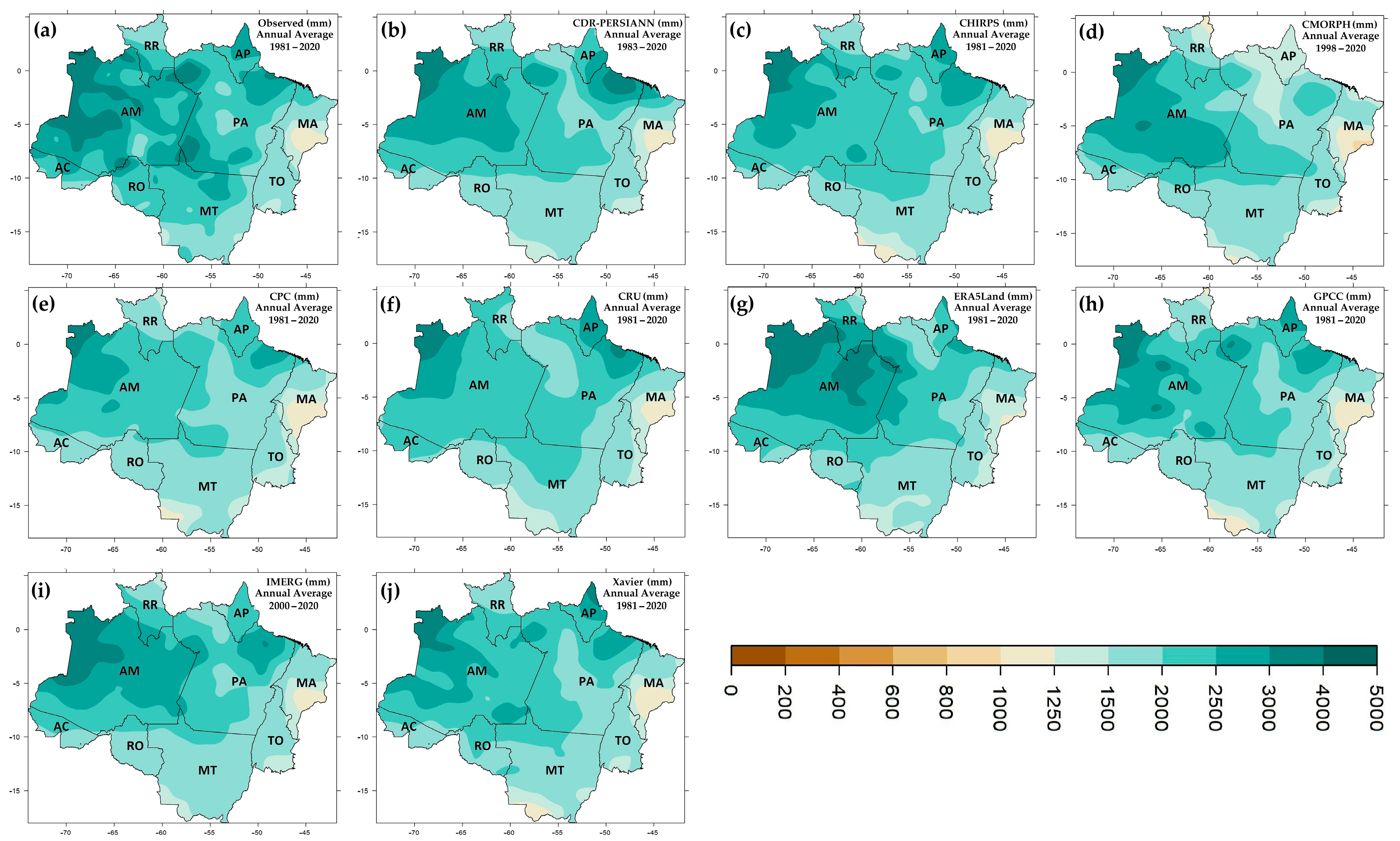
3.1. Description of the Current Climatology

Figure 3 shows the seasonal climatology for the period 1981–2020, for the quarters December–January–February (DJF, Figure 3a), March–April–May (MAM, Figure 3b), June–July–August (JJA, Figure 3c) and September–October–November (SON, Figure 3d). It can be seen that the BLA does not have a homogeneous rainfall regime: although it shows little seasonality in the far west, there is strong seasonality in the southern sector. The average annual rainfall in the BLA as a whole is around 2000 mm, ranging from 1500 mm/year in the eastern sector to 3500 mm/year in the northwest [1,86].

The BLA has almost permanent convection coupled to an equatorial low-pressure zone, which is more pronounced during DJF. In this quarter, there is a well-defined high-level anticyclone centered in Bolivia, the “Bolivian High”, which favors convection in the south–central part of the BLA and which, together with the South Atlantic Convergence Zone (SACZ), a wide and long area of mass convergence with a northwest–southeast orientation that extends from the BLA to the South Atlantic Ocean, causes significant accumulations of precipitation [87].

In MAM, convection is regulated by large-scale atmospheric circulations, including the Hadley circulation and the Intertropical Convergence Zone (ITCZ), which is responsible for most of the rainfall in the center–north of the BLA in this quarter, due to its more southerly position.

The ITCZ migrates northwards in the JJA quarter, resulting in rainfall concentrated in the far north of the BLA, benefiting the state of Roraima in particular. The center–south of the BLA experiences its driest period during this quarter [5,86,88,89,90,91,92,93].

In SON, at the height of spring in the southern hemisphere, the center–south of the BLA experiences the transition from the dry period in JJA to the rainy period in DJF, when convective activity begins and reaches its maximum in summer (DJF).

The modes of variability that most strongly influence the dynamics of Amazon rainfall are El Niño–Southern Oscillation and the sea surface temperature gradient over the tropical Atlantic, including the Caribbean Sea area [86,94,95,96,97,98].

Figure 4 comparatively shows the average annual rainfall observed in the BLA (Figure 4a) and in each database (Figure 4b–j). The western BLA is the area with the greatest accumulation of precipitation, especially in the state of Amazonas, with average accumulations that can exceed 4000 mm (Figure 4a). The lowest values are observed in the area between the states of Maranhão, most of the state of Pará, Tocantins, south–central Mato Grosso, north of Roraima and Rondônia, with annual rainfall ranging from 1000 mm to 2500 mm. This spatial feature is well captured by all data sources, and some sources have difficulty estimating the highest rainfall volume in western Amazonia, especially CPC (Figure 4e) and CRU (Figure 4f). Another area with a voluminous accumulation of annual rainfall is observed in the northern Amazon between the states of Amapá and Pará. In this area, CMOPRH (Figure 4d) and ERA5Land (Figure 4g) underestimated the observations. In general, the less rainy part of the BLA was best estimated by all data sources between the states of Maranhão and Tocantins. In the seasonal analysis, all data sources present climatologies with a spatial distribution similar to that of the observations. Figures S1–S4 in the Supplementary Material (a—Description of current climatology: seasonal analysis) show the accumulated precipitation from each data source, at the seasonal level, for the DJF, MAM, JJA and SON quarters, accompanied by a description of these results.

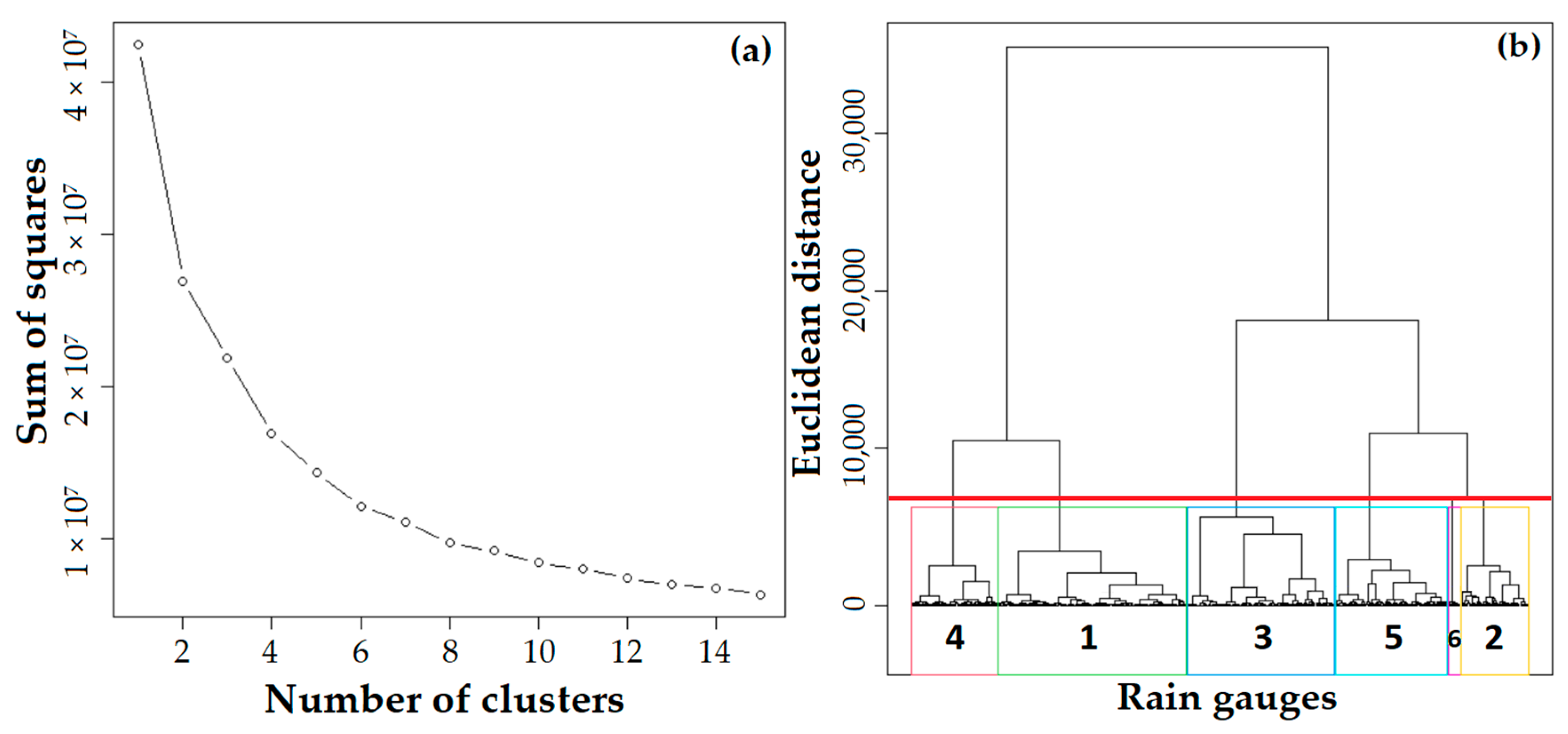
3.2. Cluster Analysis

The cluster analysis was performed with the observed monthly data, providing the division of the BLA into homogeneous precipitation regions. Six homogeneous groups were identified when the sum of squares remained approximately constant (Figure 5a). This number of groups is ideal for the subdivision of the BLA because with only six groups, it is possible to identify a very peculiar region located in the extreme north of the BLA, situated between the state of RR and the extreme northwest of the MA. This result agrees with that of [99], who tested 1 to 6 groups and only identified this homogeneous region when they subdivided the BLA into six clusters, which exceeds the BLA limits towards Venezuela according to [100].

The centroids of the points of each homogeneous region were grouped and demonstrated through a dendrogram (Figure 5b), with the respective cut-out (red line) used to divide the number of groups according to the Euclidean distance method and the hierarchical grouping by the Ward’s binding technique. The number of points belonging to each subregion is shown in

Table 2. Absolute and relative frequency of the number of stations belonging to the homogeneous subregions determined according to the monthly rainfall for the BLA.

Groups	Station Numbers	Relative Frequency	Average Annual Precipitation (mm)
1	147	30.63	1843
2	53	11,04	3055
3	115	23.96	1704
4	67	13.96	2630
5	88	18.33	2477
6	10	2.08	1899

.

Group 1 has the largest number of stations (Table 2) and covers the entire southern BLA, from the southern end of Maranhão, south-central Tocantins, part of the southeastern end of Pará, and almost all points in the Mato Grosso and Rondônia, including rain gauges in southern Acre (Figure 6a). Group 6 is the smallest group, with only 10 rainfall stations located in Roraima. The average annual rainfall observed between the stations ranges from 1704 mm (Group 3, in east–central BLA) to 3055 mm (Group 2, in west–central Amazonas).

There are marked differences in the annual cycle of each group, with strong seasonality (Figure 6b). In Group 1, rainfall is concentrated between SON and DJF, with the driest season between the groups from May to September. The Group 2 has its own characteristic among the groups, which is the short and mild dry season with an apex occurring in August, although with an accumulated average higher than 150 mm, in addition to having a monthly average higher than 250 mm from December to May. Group 3 and Group 4 have behavior similar to Group 1, with a dry season in winter and rainy season in spring–summer, although they differed in the monthly accumulated values, which are higher in Group 4 compared to Group 3, exceeding 350 mm monthly between December and March, while in Group 3 these values range from 150 mm to just over 300 mm in March, the wettest month. The dry period of Group 5 was shifted relative to Group 1, Group 2, Group 3 and Group 4 for the winter–spring months, with the rainy season concentrated in the summer–autumn, with monthly average values greater than 400 mm in March and April. The Group 6 differs from all groups, with its rainy season between late autumn and early spring, from April to September, with a peak from May to July, with average monthly rainfall above 300 mm, and a strong dry season in summer.

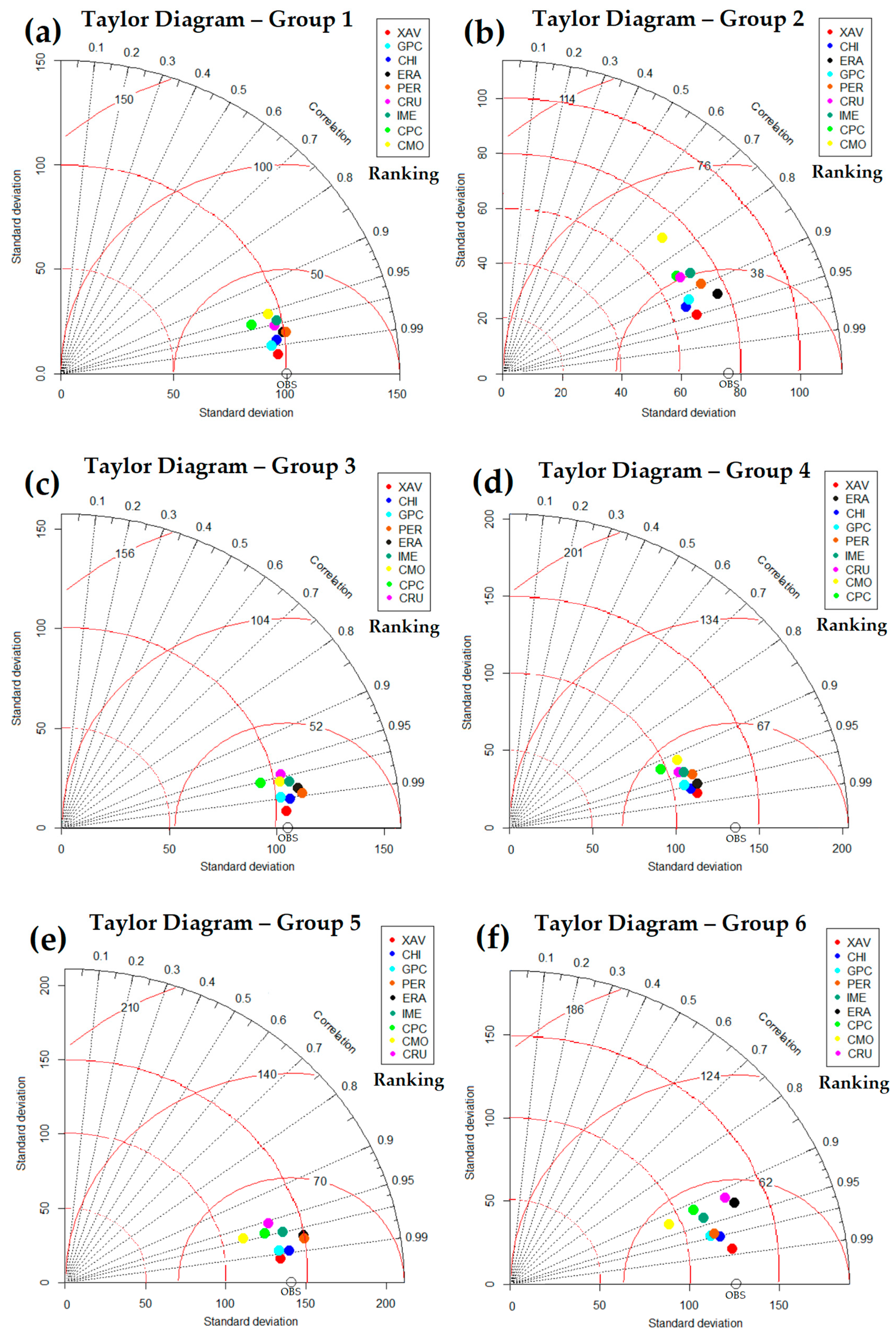
3.3. Intercomparison between Databases and Observations in BLA—Regional Analysis

In this section, we present spatial maps of three skill indices obtained from the comparison between monthly observations and estimates: bias, RMSE and correlation.

Each of these indices, individually, cannot serve as a parameter to define the main characteristics of each database and infer which of them has the best performance in BLA, so they must be analyzed together. Bias, for example, which can also be called systematic error, may not be decisive in showing such errors if positive and negative differences tend to cancel each other out.

On the other hand, high and positive correlations can be a false indicator of data quality, since considerable biases may not affect it, since it is enough for the estimated series to behave similarly to the observed one for there to be a high correlation, even with a high bias.

While the RMSE has the advantage of estimating the error of the estimate in the same unit as the variable and giving greater weight to the larger errors, due to the squared exponent that the error assumes, this metric is very sensitive to outliers (discrepant values) and, if there are many significant errors in its analysis, this metric could be extrapolated. The following subtopics, therefore, present the analysis of bias, RMSE and correlation in order to see how each result can help in the individualized assessment of the performance of each database.

3.3.1. Skill Assessment Using Bias

Figure 7 shows the consolidated monthly bias, reflecting the balance of areas with positive and negative biases observed during the seasons (see Supplementary Material), where it can be seen that on average, more regions have a predominance of underestimated precipitation, which can reach 200 mm/month in many areas of the BLA. The databases that stand out as having the most significant areas with a positive bias are the PERSIANN-CDR, CMORPH, ERA5Land and IMERGE databases (Figure 7a,c,f,h). Among all the maps, there are more areas in the BLA with slight deviations between −50 mm and 50 mm/month for CHIRPS, GPCC and Xavier (Figure 7b, Figure 7g and Figure 7i, respectively).

Figures S5–S8 in the Supplementary Material (b—Skill assessment using bias: seasonal analysis) show bias between accumulated precipitation from each data source and the respective observations for the DJF, MAM, JJA and SON quarters, accompanied by a description of these results.

3.3.2. Skill Assessment Using RMSE

In studies that involve comparisons between actual and estimated data, it is advisable to also analyze the RMSE, since it has the advantage of penalizing errors of greater magnitude, i.e., as the differences between observation and estimate increase, RMSE increases. This is useful for identifying spatial patterns that reveal where an estimate truly tends to be inaccurate.

Figure 8 shows the results of the monthly RMSE between the databases and the observation. This index has the advantage of penalizing errors of greater magnitude; i.e., as the differences between the observation and the estimate increase, the RMSE increases. This is useful for identifying spatial patterns that reveal where an estimate really tends to be inaccurate. In monthly terms, the smallest errors in shades of brown (ranging from 20 to 125 mm), for all data sources, are observed in the east of the BLA, between the states of Maranhão, Tocantins, central–eastern Pará and large portions of Mato Grosso with the exception of its southernmost tip, and in Roraima and Amapá in the extreme north of the BLA. In the west of the BLA, mainly between the states of Amazonas, southwest Pará and portions of Acre and Mato Grosso, there are the nuclei with the highest RMSE values, from 125 to 300 mm. In absolute average values, Xavier (Figure 8i) with a global average of 90 mm is the database with the lowest RMSE values, and at the other extreme is CRU (Figure 8e) with 117 mm.

Figures S9–S12 in the Supplementary Material (c—Skill assessment using RMSE: seasonal analysis) show RMSE between accumulated precipitation from each data source and the respective observations for the DJF, MAM, JJA and SON quarters, accompanied by a description of these results.

3.3.3. Comparison Using Pearson Correlation

This result shows the influence that observations have on the construction of grids, since a large part of the observed data from the ANA and INMET are used in the construction of the grid analyzed by Xavier [33], while INMET observations are used in the construction of the GPCC grid and to correct the bias of satellite estimates in CHIRPS. However, these observations are also used, for example, in the construction of the CPC and CRU grids, the latter being the data source with the worst performance in terms of correlation values in most seasons, respectively (see Supplementary Material). This performance is reflected in the overall average correlations obtained for the BLA from the spatialized data in Figure 9. Among the data sources, Xavier and GPCC (Figure 9i,g), have the highest average correlations in the area with values of 0.83 and 0.80, respectively, while CRU and ERA5Land have the lowest values, with 0.70 and 0.73, respectively.

An important feature that can be seen from the correlation fields is that the high values observed in the far north, east and south of the BLA corroborate the fact that the databases are efficient at correctly capturing seasonality, as these are the areas of the BLA where seasonality is most prominent, as shown in Figure 3. On the other hand, the lowest correlation values are observed in the area related to Group 2 (Figure 6), precisely where seasonality is more pronounced in the BLA, and rainfall is more abundant throughout the year.

Figures S13–S16 in the Supplementary Material (d—Comparison using Pearson’s correlation: seasonal analysis) show correlations between accumulated precipitation from each data source and the respective observations for the DJF, MAM, JJA and SON quarters, accompanied by a description of these results.

To help verify which sources perform best, we analyzed these parameters, summarized in Taylor diagrams below, as well as PDFs related to the homogeneous regions identified in Section 3.2.

3.4. Intercomparison between Databases and Observations in BLA on a Monthly Scale—Subregional Analysis

Figure 10 shows the Taylor diagrams for each homogeneous region, obtained from the continuous monthly time series of each database and the observation (series of the average of all the elements in each group). Although this procedure maximizes parameters such as correlation, brings the standard deviations of the observations and data sources closer together, and proportionally reduces error values, it makes it easier for us to distinguish which databases perform better compared to the observations, which are our reference on the X-axis, with SDE (Standard Deviation of the Error) = 0, r =1 and the respective standard deviation of the observation series.

It can be seen that there is a predominance of lower standard deviations of the databases compared to the observations for all groups. As σ is a measure of dispersion that indicates the degree of variation of the data around the mean, data sources with σ lower than the observation data indicate that their estimated data for the observation points of each group show less variation than the latter, which allows us to infer that these sources are less efficient at characterizing the upper extremes of their respective distributions.

The exception is the PERSIANN-CDR data in Group 1 (Figure 10a), ERA5Land in Group 2 (Figure 10b), CHIRPS, ERA5Land, PERSIANN-CDR and IMERG in Group 3 (Figure 10c), ERA5Land in Group 5 (Figure 10e), and ERA5Land and CRU in Group 6 (Figure 10f). For Group 4 (Figure 10d), all the databases tend to have a lower variance than the observations.

The dashed red lines inside the diagram in relation to the X-axis indicate the SDE values, which represent the difference between the databases and the observations, on the X-axis labeled “OBS”. Taking the distance to “OBS” as a reference for all the groups, Xavier had the lowest SDE values: 11 mm/month for Group 1, 24 mm/month for Group 2, 8 mm/month for Group 3, 32 mm/month for Group 4, 17 mm/month for Group 5 and 21 mm/month for Group 6. At the other extreme, with the highest SDE values, there was CMORPH with 32 mm/month for Group 1 and 54 mm/month for Group 2, CRU with 27 mm/month for Group 3, 42 mm/month for Group 5 and 52 mm/month for Group 6, and CPC with 58 mm/month for Group 4.

However, measures such as correlation in the Taylor diagram do not take bias into account. So to complement this information, we present relevant data from the three main parameters used in this research to identify database performance, bias, r, RMSE and the SDE obtained at seasonal and annual levels, shown in

Table 3. For each database compared to the observation, bias, Pearson’s correlation (r), RMSE and SDE obtained from the averages of the homogeneous groups in the DJF, MAM, JJA, SON quarters.

	DJF Quarter				MAM Quarter				JJA Quarter				SON Quarter
Database	bias	r	RMSE	SDE	bias	r	RMSE	SDE	bias	r	RMSE	SDE	bias	r	RMSE	SDE
Xavier	−59	0.87	77	45	−49	0.90	65	40	−20	0.91	33	23	−46	0.84	62	40
CHIRPS	−46	0.77	96	61	−33	0.87	72	52	−17	0.85	41	32	−31	0.83	58	43
GPCC	−75	0.78	96	56	−73	0.71	100	67	−41	0.79	55	36	−56	0.78	73	45
ERA5Land	2	0.73	100	70	10	0.82	101	66	−24	0.73	59	44	−12	0.69	71	57
PERSIANN-CDR	−1	0.65	106	79	−16	0.66	100	78	−16	0.81	49	38	−30	0.75	61	49
IMERG	−14	0.56	114	89	−36	0.64	99	83	−21	0.65	60	51	3	0.64	69	58
CMORPH	−110	0.61	140	77	−126	0.69	148	75	−126	0.67	132	46	39	0.74	76	51
CRU	−46	0.42	130	92	−33	0.44	123	100	−9	0.60	67	51	−38	0.56	80	62
CPC	−130	0.44	170	108	−133	0.51	169	106	−63	0.58	94	67	−82	0.48	110	72

and

Table 4. For each database compared to the observation, bias, Pearson’s correlation (r), RMSE and SDE obtained from the averages of the homogeneous groups in the in the annual period.

	Annual
Database	bias	r	RMSE	SDE
Xavier	−166	0.85	213	118
CHIRPS	−118	0.77	227	144
GPCC	−237	0.67	295	163
ERA5Land	−16	0.63	263	175
PERSIANN-CDR	−55	0.52	268	202
IMERG	−58	0.47	268	215
CMORPH	−314	0.49	395	198
CRU	−116	0.35	310	216
CPC	−396	0.22	515	316

, respectively. These values were obtained from the average of these parameters for each homogeneous group, in order to summarize this information in a single table. The higher values for some parameters such as SDE, for example, at the seasonal and annual level, are compatible with the higher accumulated values in these time intervals and, respectively, the greater differences between observed and estimated average values for each group.

On the other hand, the average values obtained for the BLA bias are more random. In the seasonal analysis shown in Table 3, it is possible to identify some databases that consistently underestimate the observed rainfall, with significant values in all quarters, such as the CPC, which is the database that most underestimates the average annual accumulated rainfall in the BLA (Table 4), followed by CMORPH, which underestimates rainfall in DJF, MAM and JJA, but overestimates it in SON. From this parameter alone, we could infer that the most accurate databases would be ERA5Land, PERSIANN-CDR and IMERG. However, it is known that considerable differences between estimates and observations can cancel each other out over a time series, which shows that this parameter, which is important, needs to be analyzed together with the other indices used to assess the performance of the databases.

The same time series used to generate and analyze the Taylor diagrams were used to generate probability density graphs and compare them with those of the observation to assess whether each source captures the basic characteristics of the observed distribution. For Group 1, Figure 11 shows the observed PDF for each month, followed by the PDFs from the other data sources. Especially in the driest months of the year, between May and August, the PDF follows a normal distribution, a characteristic that is captured relatively well by the data sources. However, in the wetter months, it is noticeable that this distribution often has bimodal, trimodal or even more biased characteristics. The CRU (Figure 11g) clearly underestimates the precipitation of the wettest months of the year. Xavier (Figure 11b) maintains PDFs that are extremely similar to the observed PDFs, as do CHIRPS and GPCC, which differ in their December bimodal distributions compared to the observed trimodal distributions, in addition to the smoothing of the January PDF that does not capture the observed trimodal behavior. ERA5Land, PERSIANN-CDR, CMORPH and IMERG differ in their PDFs from those observed in the first two months of the year, with unimodal and bimodal distributions more normalized than those observed.

Many of the characteristics described in the PDFs of Group 1 are observed for those of the other groups, which are presented and described in the Supplementary Material (Figures S17–S21) of the topic e—PDF analysis, of the other homogeneous groups (Group 2 to Group 6).

4. Discussion

This study provides a comprehensive assessment of the estimated rainfall for the BLA by nine different data sources classified into three categories: based solely on rainfall (CPC, CRU, GPCC and Xavier), based on reanalysis (ERA5Land) and based on remote sensing (CHIRPS, CMORPH, IMERG and PERSIANN-CDR), although some of these, such as CHIRPS, undergo a process of bias correction using in situ observations. From a time series of 480 observation points on the surface, duly controlled and without failures, we compared the spatial characteristics and errors of each source at monthly, seasonal and annual scales in a regional analysis, for the entire BLA, and sub-regionally, for six groups with homogeneous rainfall.

All precipitation products represent the annual cycle of precipitation in the BLA, with greater and lesser accumulation in the northwest and northeast portions. This characteristic was observed by other authors, such as [86], who evaluated eight datasets based on remote sensing versus a gridded analysis, known as HYBAM (HYdro-geochemistry of the AMazonian Basin). An important difference between our study and that of [86] is related to the observed data, in our case from 480 rainfall stations/stations that more reliably represent extremes and areas of higher/lower accumulated rainfall, i.e., we followed an inverse path, instead of comparing rainfall grids. For precipitation from satellites with a grid constructed from observations, we extracted a specific time series for each observation point from all gridded analyses using the simple bilinear interpolation method. This method allowed us to verify that despite the sources affecting the areas of highest/smallest accumulations annually and seasonally, most databases underestimate precipitation in the BLA area, with CPC and CMORPH being the sources with the highest bias precipitation in the BLA in regard to the observations, −306 mm and −304 mm, respectively, and ERA5Land and PERSIANN-CDR with the smallest differences, −125 mm and −104 mm, respectively, while ERA5Land and PERSIANN-CDR alternate in having more areas in the BLA with positive and negative biases.

The bias, as illustrated in Figure 7, is predominantly negative in several areas of the BLA, with Xavier, CHIRPS, CRU, GPCC, CPC and CMORPH standing out and the latter two databases showing the most intense negative values. Other data sources have areas of positive bias, such as PERSIANN-CDR, ERA5Land and IMERG, characterizing overestimation of precipitation. These details shown spatially are corroborated by the results in Table 4 for the average annual bias values estimated by each database for the BLA as a whole.

As illustrated in the figures for the RMSE, the largest errors are observed in central–southern Amazonas, southwestern Pará, northern and southern Mato Grosso and, for some databases such as CMORPH, in the far north in Pará and Amapá. This result was also observed in [86]. When evaluating precipitation estimated by CHIRPS for a smaller set of observations than those used in this study, Cavalcante et al. [101] found that in addition to this source underestimating precipitation in the rainiest months, it consequently underestimates extreme precipitation indices with a spatial distribution of errors similar to those found in this and other studies [86,102]. These results are corroborated by the spatial evaluation of correlations in the BLA. This parameter is fundamental for initially identifying where the best rainfall estimates come from.

As shown in Figure 9, Xavier stands out among the data sources as the one with the highest values of r, followed by GPCC and CHIRPS, while CRU and ERA5Land have observably larger areas, with correlations lower than 0.4. These results are indicative, but not yet decisive, when it comes to stating that certain databases are more efficient than others. These results were generated according to the total time of data made available by each source, i.e., for six of these we can count on 40 years, as shown in Table 1 (Xavier, CHIRPS, CPC, CRU, GPCC and ERA5Land), while we have 38 years for PERSIANN-CDR, 23 years for CMORPH and 21 years of data for IMERG. So, a direct comparison between the databases based on this spatial analysis will not be entirely honest.

Although the spatial analyses involving the entire BLA are useful in several aspects, it was necessary to subdivide this large region into smaller areas according to homogeneous groups of monthly accumulated precipitation to verify with better precision the data sources that best represent the precipitation in each subarea of the BLA. The cluster analysis showed that the BLA should be divided into six homogeneous groups called G1 to G6, like [86,99,100,103], who also used only six groups. It is possible to identify a region with climatic characteristics totally different from the others, located in the extreme north of the BLA, with a rainy season centered in winter, between the state of Roraima and extreme northwest of Amazonas (G6). Sapucci et al. [86] showed that all the remote sensing data sources used in their study allowed the identification of the same homogeneous regions as the grid analysis used as a reference, an indication that the sources represent the basic spatiotemporal characteristics of accumulated precipitation well. In our study, we assumed this premise, and for the six homogeneous groups obtained with the observations, we constructed unique time series representative of each group to better identify which group would be the most accurate in a skill ranking, based on Taylor diagrams, RMSE values, bias and correlation.

Based on the ranking position of each group, we assigned decreasing points from 10 to 2 according to the position in this ranking; for example, as there were nine data sources, for the source with greater skill in each group, it received a value score of 10, the second source a score of 9, and so on, until the last source in the ranking, which in ninth position received a score of 2, according to

Table 5. For each homogeneous group (Group 1 to Group 6), the skill ranking and respective score are relative to the position in the ranking for each data source, based on Taylor diagrams (SDE).

Ranking	Score	Group 1 (G1)	Group 2 (G2)	Group 3 (G3)	Group 4 (G4)	Group 5 (G5)	Group 6 (G6)
1	10	XAV	XAV	XAV	XAV	XAV	XAV
2	9	GPC	CHI	CHI	ERA	CHI	CHI
3	8	CHI	ERA	GPC	CHI	GPC	GPC
4	7	ERA	GPC	PER	GPC	PER	PER
5	6	PER	PER	ERA	PER	ERA	IME
6	5	CRU	CRU	IME	IME	IME	ERA
7	4	IME	IME	CMO	CRU	CPC	CPC
8	3	CPC	CPC	CPC	CMO	CMO	CMO
9	2	CMO	CMO	CRU	CPC	CRU	CRU

for Taylor diagrams,

Table 6. For each homogeneous group (Group 1 to Group 6), the skill ranking and respective score are relative to the position in the ranking for each data source, based on Pearson correlation (r).

Ranking	Score	Group 1 (G1)	Group 2 (G2)	Group 3 (G3)	Group 4 (G4)	Group 5 (G5)	Group 6 (G6)
1	10	XAV	XAV	XAV	XAV	CHI	XAV
2	9	GPC	CHI	CHI	CHI	XAV	GPC
3	8	CHI	GPC	GPC	ERA	ERA	CHI
4	7	PER	ERA	CMO	GPC	GPC	PER
5	6	ERA	PER	PER	PER	CMO	CMO
6	5	CMO	CMO	ERA	IME	PER	ERA
7	4	CRU	IME	IME	CMO	IME	CRU
8	3	IME	CRU	CRU	CPC	CPC	IME
9	2	CPC	CPC	CPC	CRU	CRU	CPC

for Pearson correlation,

Table 7. For each homogeneous group (Group 1 to Group 6), the skill ranking and respective score are relative to the position in the classification of each data source, based on the RMSE.

Ranking	Score	Group 1 (G1)	Group 2 (G2)	Group 3 (G3)	Group 4 (G4)	Group 5 (G5)	Group 6 (G6)
1	10	XAV	ERA	XAV	XAV	CHI	XAV
2	9	CHI	IME	GPC	ERA	XAV	CHI
3	8	GPC	PER	CHI	CHI	GPC	PER
4	7	CRU	CHI	CMO	IME	ERA	IME
5	6	PER	XAV	CRU	PER	IME	GPC
6	5	ERA	GPC	PER	CMO	PER	CRU
7	4	IME	CMO	ERA	CRU	CRU	ERA
8	3	CMO	CRU	IME	GPC	CPC	CMO
9	2	CPC	CPC	CPC	CPC	CMO	CPC

for RMSE and

Table 8. For each homogeneous group (Group 1 to Group 6), the skill ranking and respective score are relative to the position in the classification of each data source, based on the bias.

Ranking	Score	Group 1 (G1)	Group 2 (G2)	Group 3 (G3)	Group 4 (G4)	Group 5 (G5)	Group 6 (G6)
1	10	CHI	ERA	XAV	ERA	CRU	PER
2	9	CRU	IME	GPC	XAV	IME	IME
3	8	PER	PER	CMO	CMO	CHI	XAV
4	7	CMO	CHI	CRU	CHI	ERA	CHI
5	6	ERA	CMO	CHI	IME	XAV	CRU
6	5	XAV	XAV	ERA	PER	GPC	GPC
7	4	IME	GPC	PER	CRU	PER	CPC
8	3	GPC	CRU	IME	GPC	CPC	ERA
9	2	CPC	CPC	CPC	CPC	CMO	CMO

for bias.

For the results based on Taylor diagrams in each homogeneous region, Xavier’s gridded analysis was the source with the greatest ability to relate the observations, receiving a score of 10 for all groups. CHIRPS can be considered the second best data source, with the highest score behind Xavier in five groups (Group 2 to Group 6). GPCC had the third best overall performance and ERA5Land the fourth. In an intermediate position is PERSIANN-CDR, and occupying the last four positions in performance are IMERG, CRU, CPC and CMORPH. This ranking is easily obtained by calculating the weighted average of each source according to its score in each group. Let us look at the examples of Xavier and CHIRPS. Xavier, for occupying the first position in all groups, received the following average: Score—Xavier = (10 + 10 + 10 + 10 + 10 + 10)/6 = 10. For CHIRPS, it was the following: Score—CHIRPS = (8 + 9 + 9+9 + 9+9)/6 = 8.8, and so on. By carrying out the same procedure for the other parameters, r, RMSE and bias, we have the re-result for each parameter and the final consolidated result shown in

Table 9. Ranking of general skill among the different data sources for the BLA based on the position and respective score of each homogeneous group. The first four are highlighted in blue, the middle ones in black and the last four ones in red.

Taylor Diagrams (SDE)		Pearson Correlation (r)		RMSE		bias		Final Result
Data Source	General Score	Data Source	General Score	Data Source	General Score	Data Source	General Score	Data Source	General Score
Xavier	10.0	Xavier	9.8	Xavier	9.2	Xavier	7.2	Xavier	9.0
CHIRPS	8.7	CHIRPS	8.8	CHIRPS	8.5	CHIRPS	7.5	CHIRPS	8.4
GPCC	7.8	GPCC	8.0	GPCC	6.5	GPCC	4.8	GPCC	6.8
ERA5Land	6.8	ERA5Land	6.5	ERA5Land	6.5	ERA5Land	6.8	ERA5Land	6.7
PERSIANN	6.5	PERSIANN	6.2	PERSIANN	6.3	PERSIANN	6.5	PERSIANN	6.4
IMERG	4.8	CMORPH	5.5	IMERG	6.0	IMERG	6.7	IMERG	5.8
CRU	3.3	IMERG	3.8	CMORPH	4.0	CRU	6.5	CMORPH	4.4
CPC	3.2	CRU	3.0	CRU	4.8	CPC	2.5	CRU	3.4
CMORPH	2.8	CPC	2.3	CPC	2.2	CMORPH	5.5	CPC	3.2

, with the respective final ranking of skill between the sources based on the average of the general scores obtained in each parameter.

The results summarized in Table 9 clearly show which sources tend to estimate the accumulated average monthly rainfall most accurately in each homogeneous group, as well as in the BLA.

We expected the grid-based analysis of [33] to occupy a prominent place among the sources, because it uses a large part of the observational database we used, mainly the ANA rainfall database.

The other data sources based on gridded analysis only use data from official INMET stations that make up the Global Historical Climatology Network (GHCN) [104], as well as sources based on remote sensing but which make bias corrections using the GHCN base, such as CHIRPS and PERSIANN-CDR.

All the data sources used in this study have been the subject of studies worldwide that seek to evaluate their performance, individually or intercomparably [2,6,56,59,65,86,102,105,106,107,108,109,110,111]. In the Amazon basin, Paca et al. [98] used CHIRPS to study the variability in rainfall trends from 1981 to 2017, showing different areas with increases and decreases in this period. A similar analysis was performed by [110] for spatiotemporal rainfall trends from 1998 to 2015 in the BLA with data from the TRMM, which was integrated into the IMERG. After validating the CHIRPS for station points in the BLA, Cavalcante et al. [101] used it to investigate extreme rainfall indices, which agrees with our study in its finding that the correlations between CHIRPS and observations were considerably lower in the northwest sector of the BLA (fact found for databases investigated in this study). Sapucci et al. [86] showed that CHIRPS and PERSIANN-CDR were among the precipitation sources with the best performance for studies on the intraseasonal time scale in the Amazon basin, a result similar to those found in this study.

Unlike the study by [86], which evaluated only remote sensing sources as the main data input for grid construction, we show that there is no hierarchy of skill between gridded analyses based solely on surface observations, or coming from reanalysis or involving remote sensing. Here, we show that among the four best databases, there are two based solely on rainfall (Xavier and GPCC), one based on remote sensing but calibrated with surface observations (CHIRPS) and one from reanalysis, ERA5Land. The remotely sensed data source PERSIANN-CDR occupied an intermediate position in terms of skill among the sources, while the last four places in terms of skill also mix, as for the first four, two gridded analyses based on rainfall (CRU and CPC), one based on remote sensing (IMERG) and one based on sensing with bias correction by observations (CMORPH).

A possible explanation for the low performance of IMERG and CMORPH for most of the BLA was raised by [102], which could be attributed to the difficulty in estimating precipitation from warm clouds in the BLA [112,113,114], whose cloud top temperatures are higher than 0 °C, while the algorithms on board the sensors are calibrated to detect and estimate precipitation more easily from the duration of cold clouds, whose cloud top temperatures are lower than 0 °C.

As for CRU and CPC, we should investigate what could be behind the low performance of these two gridded analyses. One assumption is that CPC assimilates precipitation data from INMET’s automatic stations, which, when the precipitation accumulation counting sensor malfunctions, report zeros that inflate the time series for long periods, until they are detected and corrected, leading to underestimates and errors in the process of constructing a gridded analysis.

The similar performance of CPC and CMORPH is understandable, as CMORPH corrects its precipitation estimate using a probability density function based on daily CPC measurements [23,63,115]. Likewise, as shown in [115], the PERSIANN-CDR, which uses an improved version of precipitation estimation from infrared and passive microwave (PMW) satellite images of the one used by CMORPH via artificial neural networks, has its estimates adjusted by the product of the GPCC monthly rainfall to maintain its consistency and reduce bias while preserving the high spatial resolution of the daily rainfall estimates [116,117]. This may be a determining factor for the good performance that PERSIANN-CDR showed in the BLA, since the GPCC obtained the third overall performance among the nine databases evaluated.

5. Conclusions

In this study, the performances of nine databases arranged in regular grids under different spatial resolutions were evaluated compared to rainfall records from 480 stations in the BLA. The main conclusions of this study are listed as follows:

(1)

The main climatological characteristics of rainfall in the BLA are well represented by the data sources. The spatial distribution and seasonality follow the observed pattern. However, the heterogeneity of the observed patterns is not well captured, especially compared to the observed nuclei of maximum accumulated rainfall, which in the data sources tend to be smoothed out.

(2)

The BLA should be divided into six pluviometrically homogeneous regions, which facilitates the analysis of precipitation and the skill of different databases in this vast region of the planet.

(3)

There is a tendency to underestimate rainfall in the BLA.

(4)

The largest errors between database estimates are concentrated in the northwestern sector of the BLA, and the smallest in the northeastern sector.

(5)

Skill rankings based on Taylor diagrams, Pearson’s correlation and RMSE made it possible to better verify the hierarchy of skill between the different data sources compared to the observations for each homogeneous group, where it was possible to observe the good performance, especially of Xavier and CHIRPS.

(6)

Based on a skill ranking, we identified, in general, that Xavier, CHIRPS, GPCC and ERA5Land are the four sources that best represent precipitation in the BLA, with CRU and CPC in the last positions.

Although our results clearly show a degree of hierarchy based on the skill of each database in the BLA, the choice of a data source must be correlated to the type of product you want to obtain for the BLA, because there are advantages and disadvantages among all the sources mentioned, without taking into account their position in the skill ranking.

References

1. Villar, J.C.E.; Ronchail, J.; Guyot, J.L.; Cochonneau, G.; Naziano, F.; Lavado, W.; Oliveira, E.; Pombosa, R.; Vauchel, P. Spatio-temporal rainfall variability in the Amazon basin countries (Brazil, Peru, Bolivia, Colombia, and Ecuador). Int. J. Climatol. 2009, 29, 1574–1594. [Google Scholar] [CrossRef]
2. Paccini, L.; Espinoza, J.C.; Ronchail, J.; Segura, H. Intra-seasonal rainfall variability in the Amazon basin related to large-scale circulation patterns: A focus on western Amazon–Andes transition region. Int. J. Climatol. 2017, 38, 2386–2399. [Google Scholar] [CrossRef]
3. Cohen, J.C.P.; Dias, M.A.F.S.; Nobre, C.A. Environmental conditions associated with amazonian squall lines: A case study. Mon. Weather Rev. 1995, 123, 3163–3174. [Google Scholar] [CrossRef]
4. Alcântara, C.; Dias, M.A.F.S.; Souza, E.P.; Cohen, J.C.P. Verification of the role of the low level jets in Amazon squall lines. Atmos. Res. 2011, 100, 36–44. [Google Scholar] [CrossRef]
5. Vizy, E.K.; Cook, K.H. Relationship between Amazon and high Andes rainfall. J. Geophys. Res. 2007, 112, 1–14. [Google Scholar] [CrossRef]
6. Segura, H.; Espinoza, J.C.; Junquas, C.; Lebel, T.; Vuille, M.; Garreaud, R. Recent changes in the precipitation-driving processes over the southern tropical Andes/western Amazon. Clim. Dyn. 2020, 54, 2613–2631. [Google Scholar] [CrossRef]
7. Xu, D.; Agee, E.; Wang, J.; Ivanov, V.Y. Estimation of evapotranspiration of Amazon rainforest using the maximum entropy production method. Geophys. Res. Lett. 2019, 46, 1402–1412. [Google Scholar] [CrossRef]
8. O’Connor, J.; Santos, M.J.; Rebel, K.T.; Dekker, S.C. The influence of water table depth on evapotranspiration in the Amazon arc of deforestation. Hydrol. Earth Syst. Sci. 2019, 23, 3917–3931. [Google Scholar] [CrossRef]
9. Drumond, A.; Marengo, J.; Ambrizzi, T.; Nieto, R.; Moreira, L.; Gimeno, L. The role of the Amazon Basin moisture in the atmospheric branch of the hydrological cycle: A Lagrangian analysis. Hydrol. Earth Syst. Sci. 2014, 18, 2577–2598. [Google Scholar] [CrossRef]
10. Carvalho, L.M.V. Assessing precipitation trends in the Americas with historical data: A review. WIREs Clim. Chang. 2020, 11, e627. [Google Scholar] [CrossRef]
11. Lucas, E.W.M.; Sousa, F.A.S.; Silva, F.D.S.; da Rocha Júnior, R.L.; Pinto, D.D.C.; Silva, V.P.R. Trends in climate extreme indices assessed in the Xingu river basin-Brazilian Amazon. Weather Clim. Extrem. 2021, 31, 100306. [Google Scholar] [CrossRef]
12. Mishra, A.K. Effect of rain gauge density over the accuracy of rainfall: A case study over Bangalore, India. Springer Plus 2013, 2, 311. [Google Scholar] [CrossRef]
13. Xu, H.; Xu, C.-Y.; Chen, H.; Zhang, Z.; Li, L. Assessing the influence of rain gauge density and distribution on hydrological model performance in a humid region of China. J. Hydrol. 2013, 505, 1–12. [Google Scholar] [CrossRef]
14. López, M.G.; Wennerstrom, H.; Norden, L.; Seibert, J. Location and density of rain gauges for the estimation of spatial varying precipitation. Geogr. Ann. Ser. A Phys. Geogr. 2015, 97, 167–179. [Google Scholar] [CrossRef]
15. Tiwari, S.; Jha, S.K.; Singh, A. Quantification of node importance in rain gauge network: Influence of temporal resolution and rain gauge density. Sci. Rep. 2020, 10, 9761. [Google Scholar] [CrossRef] [PubMed]
16. Liebmann, B.; Allured, D. Daily Precipitation Grids for South America. Bull. Am. Meteorol. Soc. 2005, 86, 1567–1570. [Google Scholar] [CrossRef]
17. New, M.; Hulme, M.; Jones, P. Representing Twentieth-Century Space Time Climate Variability. Part II: Development of 1901–1996 Monthly Grids of Terrestrial Surface Climate. J. Clim. 2000, 13, 2217–2238. [Google Scholar] [CrossRef]
18. Brands, S.; Gutiérrez, J.M.; Herrera, S. On the Use of Reanalysis Data for Downscaling. J. Clim. 2012, 25, 2517–2526. [Google Scholar] [CrossRef]
19. Xavier, A.C.; King, C.W.; Scanlon, B.R. Daily gridded meteorological variables in brazil (1980–2013). Int. J. Climatol. 2016, 36, 2644–2659. [Google Scholar] [CrossRef]
20. Xie, P.; Arkin, P.A. Global Precipitation: A 17-Year Monthly Analysis Based on Gauge Observations, Satellite Estimates, and Numerical Model Outputs. Bull. Am. Meteorol. Soc. 1997, 78, 2539–2558. [Google Scholar] [CrossRef]
21. Huffman, G.J.; Adler, R.F.; Morrissey, M.M.; Bolvin, D.T.; Curtis, S.; Joyce, R.; McGavock, B.; Susskind, J. Global Precipitation at One-Degree Daily Resolution from Multisatellite Observations. J. Hydrometeorol. 2001, 2, 36–50. [Google Scholar] [CrossRef]
22. Adler, R.F.; Huffman, G.J.; Chang, A.; Ferraro, R.; Xie, P.-P.; Janowiak, J.; Rudolf, B.; Schneider, U.; Curtis, S.; Bolvin, D.; et al. The Version-2 Global Precipitation Climatology Project (GPCP) Monthly Precipitation Analysis (1979–Present). J. Hydrometeorol. 2003, 4, 1147–1167. [Google Scholar] [CrossRef]
23. Joyce, R.J.; Janowiak, J.E.; Arkin, P.A.; Xie, P. CMORPH: A Method That Produces Global Precipitation Estimates from Passive Microwave and Infrared Data at High Spatial and Temporal Resolution. J. Hydrometeorol. 2004, 5, 487–503. [Google Scholar] [CrossRef]
24. Levizzani, V.; Bauer, P.; Turk, F.J. Measuring Precipitation from Space. Advances in Global Change Research; Springer: Dordrecht, The Netherlands; Berlin/Heidelberg, Germany, 2007; 724p. [Google Scholar]
25. Becker, A.; Finger, P.; Meyer-Christoffer, A.; Rudolf, B.; Schamm, K.; Schneider, U.; Ziese, M. A description of the global land-surface precipitation data products of the Global Precipitation Climatology Centre with sample applications including centennial (trend) analysis from 1901–present. Earth Syst. Sci. Data 2013, 5, 71–99. [Google Scholar] [CrossRef]
26. Funk, C.; Peterson, P.; Landsfeld, M.; Pedreros, D.; Verdin, J.; Shukla, S.; Husak, G.; Rowland, J.; Harrison, L.; Hoell, A.; et al. The climate hazards infrared precipitation with stations: A new environmental record for monitoring extremes. Sci. Data 2015, 2, 150066. [Google Scholar] [CrossRef] [PubMed]
27. Tapiador, F.J.; Navarro, A.; Jimenéz, A.; Moreno, R.; García-Ortega, E. Discrepancies with satellite observations in the spatial structure of global precipitation as derived from global climate models. Q. J. R. Meteorol. Soc. 2018, 144, 419–435. [Google Scholar] [CrossRef]
28. Sheffield, J.; Goteti, G.; Wood, E.F. Development of a 50-Year High-Resolution Global Dataset of Meteorological Forcings for Land Surface Modeling. J. Clim. 2006, 19, 3088–3111. [Google Scholar] [CrossRef]
29. Kalnay, E.; Kanamitsu, M.; Kistler, R.; Collins, W.; Deaven, D.; Gandin, L.; Iredell, M.; Saha, S.; White, G.; Woollen, J.; et al. The NCEP/NCAR 40-Year Reanalysis Project. Bull. Am. Meteorol. Soc. 1996, 77, 437–472. [Google Scholar] [CrossRef]
30. Veríssimo, A.; Rolla, A.; Vedoveto, M.; Futada, S.M. Áreas Protegidas na Amazônia BRASILEIRA Avanços e Desafios; IMAZON/ISA: Belém, Brazil, 2011; Available online: https://imazon.org.br/areas-protegidas-na-amazonia-brasileira-avancos-e-desafios-2/ (accessed on 23 October 2023).
31. Herdies, D.L.; Silva, F.D.d.S.; Gomes, H.B.; Silva, M.C.L.d.; Gomes, H.B.; Costa, R.L.; Lins, M.C.C.; Reis, J.S.d.; Kubota, P.Y.; Souza, D.C.d.; et al. Evaluation of Surface Data Simulation Performance with the Brazilian Global Atmospheric Model (BAM). Atmosphere 2023, 14, 125. [Google Scholar] [CrossRef]
32. Costa, R.L.; Gomes, H.B.; Pinto, D.D.C.; da Rocha Júnior, R.L.; dos Santos Silva, F.D.; Gomes, H.B.; da Silva, M.C.L.; Herdies, D.L. Gap Filling and Quality Control Applied to Meteorological Variables Measured in the Northeast Region of Brazil. Atmosphere 2021, 12, 1278. [Google Scholar] [CrossRef]
33. Xavier, A.C.; Scanlon, B.R.; King, C.W.; Alves, A.I. New improved Brazilian daily weather gridded data (1961–2020). Int. J. Climatol. 2022, 42, 8390–8404. [Google Scholar] [CrossRef]
34. Silva, J.S.; Cabral Júnior, J.B.; Rodrigues, D.T.; Silva, F.D.S. Climatology and significant trends in air temperature in Alagoas, Northeast Brazil. Theor. Appl. Climatol. 2023, 151, 1805–1824. [Google Scholar] [CrossRef]
35. da Rocha Júnior, R.L.; dos Santos Silva, F.D.; Lisboa Costa, R.; Barros Gomes, H.; Herdies, D.L.; Rodrigues da Silva, V.d.P.; Candido Xavier, A. Analysis of the Space–Temporal Trends of Wet Conditions in the Different Rainy Seasons of Brazilian Northeast by Quantile Regression and Bootstrap Test. Geosciences 2019, 9, 457. [Google Scholar] [CrossRef]
36. Paredes-Trejo, F.; Barbosa, H.A.; dos Santos, C.A.C. Evaluation of the Performance of SM2RAIN-Derived Rainfall Products over Brazil. Remote Sens. 2019, 11, 1113. [Google Scholar] [CrossRef]
37. Silva, P.E.; Spyrides, M.H.C.; Barbosa, L.M. Analysis of Climate Extreme Indices in the Northeast Brazil and the Brazilian Amazon in the Period from 1980 to 2013. Anuário Inst. Geociências 2019, 42, 137–148. [Google Scholar] [CrossRef]
38. dos Reis, L.C.; Silva, C.M.S.; Silva, C.M.S.; Bezerra, B.G.; Mutti, P.R.; Spyrides, M.H.C.; da Silva, P.E. Analysis of Climate Extreme Indices in the MATOPIBA Region, Brazil. Pure Appl. Geophys. 2020, 177, 4457–4478. [Google Scholar] [CrossRef]
39. Cressman, G.P. An operational objective analysis system. Mon. Weather Rev. 1959, 87, 367–374. [Google Scholar] [CrossRef]
40. Glahn, H.R.; Chambers, T.L.; Richardson, W.S.; Perrotti, H.P. Objective Map Analysis for the Local AFOS MOS Program; NOAA Technical Memorandum; National Weather Service TDL 75; Techniques Development Laboratory: Silver Spring, MD, USA, 1985; 34p. [Google Scholar]
41. Charba, J.P.; Harrell, A.W., III; Lackner, A.C., III. A Monthly Precipitation Amount Climatology Derived from Published Atlas Maps: Development of a Digital Database; National Oceanic and Atmospheric Administration TDL Office Note 92-7; Techniques Development Laboratory: Silver Spring, MD, USA, 1992; 20p. [Google Scholar]
42. Silva, V.B.S.; Kousky, V.E.; Shi, W.; Higgins, R.W. An Improved Gridded Historical Daily Precipitation Analysis for Brazil. J. Hydrometeorol. 2007, 8, 847–861. [Google Scholar] [CrossRef]
43. Chen, M.; Shi, W.; Xie, P.; Silva, V.B.S.; Kousky, V.E.; Higgins, R.W.; Janowiak, J.E. Assessing objective techniques for gauge-based analyses of global daily precipitation. J. Geophys. Res.-Atmos. 2008, 113. [Google Scholar] [CrossRef]
44. Basheer, M.; Elagib, N.A. Performance of satellite-based and GPCC 7.0 rainfall products in an extremely data-scarce country in the Nile Basin. Atmos. Res. 2016, 215, 128–140. [Google Scholar] [CrossRef]
45. Schneider, U.; Ziese, M.; Meyer-Christoffer, A.; Finger, P.; Rustemeier, E.; Becker, A. The new portfolio of global precipitation data products of the Global Precipitation Climatology Centre suitable to assess and quantify the global water cycle and resources. Proc. IAHS 2016, 374, 29–34. [Google Scholar] [CrossRef]
46. Harris, I.; Osborn, T.J.; Jones, P.; Lister, D. Version 4 of the CRU TS monthly high-resolution gridded multivariate climate dataset. Sci. Data 2020, 7, 109. [Google Scholar] [CrossRef]
47. Dee, D.P.; Uppala, S.M.; Simmons, A.J.; Berrisford, P.; Poli, P.; Kobayashi, S.; Andrae, U.; Balmaseda, M.A.; Balsamo, G.; Bauer, P.; et al. The ERA-Interim reanalysis: Configuration and performance of the data assimilation system. Q. J. R. Meteorol. Soc. 2011, 137, 553–597. [Google Scholar] [CrossRef]
48. Balsamo, G.; Albergel, C.; Beljaars, A.; Boussetta, S.; Brun, E.; Cloke, H.; Dee, D.; Dutra, E.; Muñoz-Sabater, J.; Pappenberger, F.; et al. ERA-Interim/Land: A global land surface reanalysis data set. Hydrol. Earth Syst. Sci. 2015, 19, 389–407. [Google Scholar] [CrossRef]
49. Uppala, S.M.; Kallberg, P.W.; Simmons, A.J.; Andrae, U.; Bechtold, V.C.; Fiorino, M.; Gibson, J.K.; Haseler, J.; Hernandez, A.; Kelly, G.A.; et al. The ERA-40 re-analysis. Q. J. R. Meteorol. Soc. 2005, 131, 2961–3012. [Google Scholar] [CrossRef]
50. Muñoz Sabater, J.; Dutra, E.; Agustí-Panareda, A.; Albergel, C.; Arduini, G.; Balsamo, G.; Boussetta, S.; Choulga, M.; Harrigan, S.; Hersbach, H.; et al. ERA5-Land: A state-of-the-art global reanalysis dataset for land applications. ESSD Discuss. 2021, 13, 4349–4383. [Google Scholar] [CrossRef]
51. Hersbach, H.; Bell, B.; Berrisford, P.; Hirahara, S.; Horányi, A.; Muñoz-Sabater, J.; Nicolas, J.; Peubey, C.; Radu, R.; Schepers, D.; et al. The ERA5 global reanalysis. Q. J. R. Meteorol. Soc. 2020, 146, 1999–2049. [Google Scholar] [CrossRef]
52. New, M.; Hulme, M.; Jones, P. Representing Twentieth-Century Space-Time Climate Variability. Part I: Development of a 1961–90 Mean Monthly Terrestrial Climatology. J. Clim. 1999, 12, 829–856. [Google Scholar] [CrossRef]
53. Schneider, U.; Becker, A.; Finger, P.; Meyer-Christoffer, A.; Ziese, M.; Rudolf, B. GPCC’s new land surface precipitation climatology based on quality-controlled in situ data and its role in quantifying the global water cycle. Theor. Appl. Climatol. 2013, 115, 15–40. [Google Scholar] [CrossRef]
54. Huffman, G.J.; Bolvin, D.T.; Nelkin, E.J.; Wolff, D.B.; Adler, R.F.; Gu, G.; Hong, Y.; Bowman, K.O.; Stocker, E.F. The TRMM Multisatellite Precipitation Analysis (TMPA): Quasi-Global, Multiyear, Combined-Sensor Precipitation Estimates at Fine Scales. J. Hydrometeorol. 2007, 8, 38–55. [Google Scholar] [CrossRef]
55. Hou, A.Y.; Kakar, R.K.; Neeck, S.; Azarbarzin, A.A.; Kummerow, C.D.; Kojima, M.; Oki, R.; Nakamura, K.; Iguchi, T. The global precipitation measurement mission. Bull. Am. Meteorol. Soc. 2014, 95, 701–722. [Google Scholar] [CrossRef]
56. Sharifi, E.; Steinacker, R.; Saghafian, B. Assessment of GPM-IMERG and Other Precipitation Products against Gauge Data under Different Topographic and Climatic Conditions in Iran: Preliminary Results. Remote Sens. 2016, 8, 135. [Google Scholar] [CrossRef]
57. Liu, Z. Comparison of versions 6 and 7 3-hourly TRMM multi-satellite precipitation analysis (TMPA) research products. Atmos. Res. 2015, 163, 91–101. [Google Scholar] [CrossRef]
58. Tang, G.; Ma, Y.; Long, D.; Zhong, L.; Hong, Y. Evaluation of GPM Day-1 IMERG and TMPA Version-7 legacy products over Mainland China at multiple spatiotemporal scales. J. Hydrol. 2016, 533, 152–167. [Google Scholar] [CrossRef]
59. Ramsauer, T.; Weib, T.; Marzahn, P. Comparison of the GPM IMERG Final Precipitation Product to RADOLAN Weather Radar Data over the Topographically and Climatically Diverse Germany. Remote Sens. 2018, 10, 2029. [Google Scholar] [CrossRef]
60. Huffman, G.J.; Bolvin, D.T.; Braithwaite, D.; Hsu, K.L.; Joyce, R.J.; Kidd, C.; Nelkin, E.J.; Sorooshian, S.; Stocker, E.F.; Tan, J. Integrated multi-satellitE retrievals for the global precipitation measurement (GPM) mission (IMERG) [Dataset]. Satell. Precip. Meas. 2020, 1, 343–353. [Google Scholar]
61. Rozante, J.R.; Gutierrez, E.R.; Fernandes, A.A.; Vila, D.A. Performance of precipitation products obtained from combinations of satellite and surface observations. Int. J. Remote Sens. 2020, 41, 7585–7604. [Google Scholar] [CrossRef]
62. Haile, A.T.; Habib, E.; Rientjes, T. Evaluation of the climate prediction center (CPC) morphing technique (CMORPH) rainfall product on hourly time scales over the source of the Blue Nile River. Hydrol. Process. 2013, 27, 1829–1839. [Google Scholar] [CrossRef]
63. Xie, P.; Joyce, R.; Wu, S.; Yoo, S.-H.; Yarosh, Y.; Sun, F.; Lin, R. Reprocessed, Bias-Corrected CMORPH Global High-Resolution Precipitation Estimates from 1998. J. Hydrometeorol. 2017, 18, 1617–1641. [Google Scholar] [CrossRef]
64. Jiang, Q.; Li, W.; Wen, J.; Qiu, C.; Sun, W.; Fang, Q.; Xu, M.; Tan, J. Accuracy evaluation of two high-resolution satellite-based rainfall products: TRMM 3B42V7 and CMORPH in Shanghai. Water 2018, 10, 40. [Google Scholar] [CrossRef]
65. Bruster-Flores, J.L.; Ortiz-Gómez, R.; Ferriño-Fierro, A.L.; Guerra-Cobián, V.H.; Burgos-Flores, D.; Lizárraga-Mendiola, L.G. Evaluation of Precipitation Estimates CMORPH-CRT on Regions of Mexico with Different Climates. Water 2019, 11, 1722. [Google Scholar] [CrossRef]
66. Pingping, X.; Joyce, R.; Wu, S.; Yoo, S.-H.; Yarosh, Y.; Sun, F.; Lin, R. NOAA Climate Data Record (CDR) of CPC Morphing Technique (CMORPH) High Resolution Global Precipitation Estimates, Version 1; National Centers for Environmental Information: Asheville, NC, USA, 2019. [Google Scholar]
67. Rossow, W.B.; Tselioudis, G.; Polak, A.; Jakob, C. Tropical climate described as a distribution of weather states indicated by distinct mesoscale cloud property mixtures. Geophys. Res. Lett. 2005, 32, L21812. [Google Scholar] [CrossRef]
68. Knapp, K.R. Scientific data stewardship of International Satellite Cloud Climatology Project B1 global geostationary observations. J. Appl. Remote Sens. 2008, 2, 023548. [Google Scholar] [CrossRef]
69. Knapp, K.R.; Ansari, S.; Bain, C.L.; Bourassa, M.A.; Dickinson, M.J.; Funk, C.; Helms, C.N.; Hennon, C.C.; Holmes, C.D.; Huffman, G.J.; et al. Globally gridded satellite observations for climate studies. Bull. Am. Meteor. Soc. 2011, 92, 893–907. [Google Scholar] [CrossRef]
70. Ashouri, H.; Hsu, K.-L.; Sorooshian, S.; Braithwaite, D.K.; Knapp, K.R.; Cecil, L.D.; Nelson, B.R.; Prat, O.P. PERSIANN-CDR: Daily Precipitation Climate Data Record from Multisatellite Observations for Hydrological and Climate Studies. Bull. Am. Meteorol. Soc. 2015, 96, 69–83. [Google Scholar] [CrossRef]
71. Sadeghi, M.; Asanjan, A.A.; Faridzad, M.; Nguyen, P.; Hsu, K.; Sorooshian, S.; Braithwaite, D. PERSIANN-CNN: Precipitation Estimation from Remotely Sensed Information Using Artificial Neural Networks–Convolutional Neural Networks. J. Hydrometeorol. 2019, 20, 2273–2289. [Google Scholar] [CrossRef]
72. Mosaffa, H.; Sadeghi, M.; Hayatbini, N.; Gorooh, V.A.; Asanjan, A.A.; Nguyen, P.; Sorooshian, S. Spatiotemporal Variations of Precipitation over Iran Using the High-Resolution and Nearly Four Decades Satellite-Based PERSIANN-CDR Dataset. Remote Sens. 2020, 12, 1584. [Google Scholar] [CrossRef]
73. Wang, J.; Petersen, W.A.; Wolff, D.B. Validation of Satellite-Based Precipitation Products from TRMM to GPM. Remote Sens. 2021, 13, 1745. [Google Scholar] [CrossRef]
74. Lyra, G.B.; Oliveira Júnior, J.F.; Zeri, M. Cluster analysis applied to the spatial and temporal variability of monthly rainfall in Alagoas state, Northeast of Brazil. Int. J. Climatol. 2014, 34, 3546–3558. [Google Scholar] [CrossRef]
75. Santos, C.A.G.; Brasil Neto, R.M.; Silva, R.M.; Costa, S.G.F. Cluster Analysis Applied to Spatiotemporal Variability of Monthly Precipitation over Paraíba State Using Tropical Rainfall Measuring Mission (TRMM) Data. Remote Sens. 2019, 11, 637. [Google Scholar] [CrossRef]
76. Costa, R.L.; de Mello Baptista, G.M.; Barros Gomes, H.; dos Santos Silva, F.D.; da Rocha Júnior, R.L.; de Araújo Salvador, M.; Herdies, D.L. Analysis of climate extremes indices over northeast Brazil from 1961 to 2014. Weather Clim. Extrem. 2020, 28, 100254. [Google Scholar] [CrossRef]
77. Mimmack, G.M.; Mason, S.J.; Galpin, J.S. Choice of distance matrices in cluster analysis: Defining regions. J. Clim. 2001, 14, 2790–2797. [Google Scholar] [CrossRef]
78. Ward, J.H. Hierarchical grouping to optimize an objective function. J. Am. Stat. Assoc. 1963, 58, 236–244. [Google Scholar] [CrossRef]
79. Hervada-Sala, C.; Jarauta-Bragulat, E. A program to perform Ward’s clustering method on several regionalized variables. Comput. Geosci. 2004, 30, 881–886. [Google Scholar] [CrossRef]
80. Liu, B.; Liu, F.; Wang, C.; Mei, S. Unit commitment considering flexibility and uncertainty of wind power generation. Power Syst. Technol. 2015, 39, 730–736. [Google Scholar]
81. Silva, E.H.d.L.; Silva, F.D.d.S.; Junior, R.S.d.S.; Pinto, D.D.C.; Costa, R.L.; Gomes, H.B.; Júnior, J.B.C.; de Freitas, I.G.F.; Herdies, D.L. Performance Assessment of Different Precipitation Databases (Gridded Analyses and Reanalyses) for the New Brazilian Agricultural Frontier: SEALBA. Water 2022, 14, 1473. [Google Scholar] [CrossRef]
82. Demirtas, M.; Nance, L.; Barnardet, L.; Lin, Y.; Chuang, H.-Y.; Loughe, A.; Mahoney, J.; Gall, R.; Koch, S. The Developmental Testbed Center Verification System; WRF/MM5 Users’ Workshop; NCAR: Boulder, CO, USA, 2005. [Google Scholar]
83. Michot, V.; Vila, D.; Arvor, D.; Corpetti, T.; Ronchail, J.; Funatsu, B.M.; Dubreuil, V. Performance of TRMM TMPA 3B42 V7 in Replicating Daily Precipitation and Regional Precipitation Regimes in the Amazon Basin (1998–2013). Remote Sens. 2018, 10, 1879. [Google Scholar] [CrossRef]
84. Rodrigues, D.T.; Silva, C.M.S.; Reis, J.S.; Palharini, R.S.A.; Cabral Júnior, J.B.; Silva, H.J.F.; Mutti, P.R.; Bezerra, B.G.; Gonçalves, W.A. Evaluation of the Integrated Multi-SatellitE Retrievals for the Global Precipitation Measurement (IMERG) Product in the São Francisco Basin (Brazil). Water 2021, 13, 2714. [Google Scholar] [CrossRef]
85. Wadoux, A.M.J.-C.; Walvoort, D.J.J.; Brus, D.J. An integrated approach for the evaluation of quantitative soil maps through Taylor and solar diagrams. Geoderma 2022, 405, 115332. [Google Scholar] [CrossRef]
86. Sapucci, C.R.; Mayta, V.C.; Dias, P.L.S. Evaluation of diverse-based precipitation data over the Amazon Region. Theor. Appl. Climatol. 2022, 149, 1167–1193. [Google Scholar] [CrossRef]
87. Ambrizzi, T.; Ferraz, S.E.T. An objective criterion for determining the South Atlantic Convergence Zone. Front. Environ. Sci. 2015, 3, 23. [Google Scholar] [CrossRef]
88. Hastenrath, S.; Heller, L. Dynamics of climatic hazards in Northeast Brazil. Q. J. R. Meteorol. Soc. 1977, 103, 77–92. [Google Scholar] [CrossRef]
89. Nobre, P.; Shukla, J. Variation of sea surface temperature, wind stress and rainfall over the tropical Atlantic and South America. J. Clim. 1996, 9, 2464–2479. [Google Scholar] [CrossRef]
90. Souza, E.B.; Alves, J.M.B.; Nobre, P. Anomalias de precipitação nos setores norte e leste do Nordeste Brasileiro em associação aos eventos do Padrão de Dipolo observados sobre o Atlântico Tropical. Rev. Bras. Meteorol. 1998, 13, 45–56. [Google Scholar]
91. Xavier, T.M.B.S.; Xavier, A.F.S.; Dias, P.L.S.; Dias, M.A.F.S. A Zona de Convergência Intertropical e suas relações com a chuva do Ceará (1964–98). Rev. Bras. Meteorol. 2000, 15, 27–43. [Google Scholar]
92. Souza, E.B.; Kayano, M.T.; Ambrizzi, T. The regional precipitation over the eastern Amazon/Northeast Brazil modulated by tropical Pacific and Atlantic SST anomalies on weekly timescale. Rev. Bras. Meteorol. 2004, 19, 113–122. [Google Scholar]
93. Wang, H.; Fu, R. The Influence of Amazon Rainfall on the Atlantic ITCZ through Convectively Coupled Kelvin Waves. J. Clim. 2007, 20, 1188–1201. [Google Scholar] [CrossRef]
94. Marengo, J.A.; Druyan, L.M.; Hastenrath, S. Observational and modelling studies of Amazonia interannual climate variability. Clim. Chang. 1993, 23, 267–286. [Google Scholar] [CrossRef]
95. Penland, C.; Matrosova, L. Prediction of Tropical Atlantic Sea Surface Temperatures Using Linear Inverse Modeling. J. Clim. 1998, 11, 483–496. [Google Scholar] [CrossRef]
96. Chérubin, L.M.; Richardson, P.L. Caribbean current variability and the influence of the Amazon and Orinoco freshwater plumes. Deep Sea Res. Part I Oceanogr. Res. Pap. 2007, 54, 1451–1473. [Google Scholar] [CrossRef]
97. Yoon, J.H.; Zeng, N. An Atlantic Influence on Amazon Rainfall. Clim. Dyn. 2010, 34, 249–264. [Google Scholar] [CrossRef]
98. Paca, V.H.M.; Espinoza-Dávalos, G.E.; Moreira, D.M.; Comair, G. Variability of Trends in Precipitation across the Amazon River Basin Determined from the CHIRPS Precipitation Product and from Station Records. Water 2020, 12, 1244. [Google Scholar] [CrossRef]
99. Santos, E.B.; Lucio, P.S.; Santos e Silva, C.M. Precipitation regionalization of the Brazilian Amazon. Atmos. Sci. Lett. 2015, 16, 185–192. [Google Scholar] [CrossRef]
100. Villa, P.M.; Moraes, J.R.S.C.; Martorano, L.G.; Martins, S.V.; Rodrigues, A.L.; Gonzáles, B.; Rolim, G.S.; Silva, A.S. Spatio-Temporal variability of precipitation in the Venezuelan region. Rev. Bras. Climatol. 2021, 9, 626–649. [Google Scholar]
101. Cavalcante, R.B.L.; Ferreira, D.B.S.; Pontes, P.R.M.; Tedeschi, R.G.; Costa, C.P.W.; Souza, E.B. Evaluation of extreme rainfall indices from CHIRPS precipitation estimates over the Brazilian Amazonia. Atmos. Res. 2020, 238, 104879. [Google Scholar] [CrossRef]
102. Funatsu, B.M.; Le Roux, R.; Arvor, D.; Espinoza, J.C.; Claud, C.; Ronchail, J.; Michot, V.; Dubreuil, V. Assessing precipitation extremes (1981–2018) and deep convective activity (2002–2018) in the Amazon region with CHIRPS and AMSU data. Clim. Dyn. 2021, 57, 827–849. [Google Scholar] [CrossRef]
103. Barni, P.E.; Barbosa, R.I.; Xaud, H.A.M.; Xaud, M.R.; Fearnside, P.M. Precipitation in northern Amazonia: Spatial distribution in Roraima, Brazil. Soc. Nat. 2020, 32, 439–456. [Google Scholar] [CrossRef]
104. Vose, R.S.; Applequist, S.; Squires, M.; Durre, I.; Menne, M.J.; Williams, C.N., Jr.; Fenimore, C.; Gleason, K.; Arndt, D. Improved Historical Temperature and Precipitation Time Series for U.S. Climate Divisions. J. Appl. Meteorol. Climatol. 2014, 53, 1232–1251. [Google Scholar] [CrossRef]
105. Medina, F.D.; Zossi, B.S.; Bossolasco, A.; Elias, A.G. Performance of CHIRPS dataset for monthly and annual rainfall-indices in Northern Argentina. Atmos. Res. 2022, 283, 106545. [Google Scholar] [CrossRef]
106. Moazami, S.; Najafi, M.R. A comprehensive evaluation of GPM-IMERG V06 and MRMS with hourly ground-based precipitation observations across Canada. J. Hydrol. 2021, 594, 125929. [Google Scholar] [CrossRef]
107. Helmi, A.M.; Abdelhamed, M.S. Evaluation of CMORPH, PERSIANN-CDR, CHIRPS V2.0, TMPA 3B42 V7, and GPM IMERG V6 Satellite Precipitation Datasets in Arabian Arid Regions. Water 2023, 15, 92. [Google Scholar] [CrossRef]
108. Schneider, U.; Finger, P.; Meyer-Christoffer, A.; Rustemeier, E.; Ziese, M.; Becker, A. 2017. Evaluating the hydrological cycle over land using the newly-corrected precipitation climatology from the Global Precipitation Climatology Centre (GPCC). Atmosphere 2017, 8, 52. [Google Scholar] [CrossRef]
109. Sadeghi, M.; Nguyen, P.; Naeini, M.R.; Hsu, K.; Braithwaite, D.; Sorooshian, S. PERSIANN-CCS-CDR, a 3-hourly 0.04° global precipitation climate data record for heavy precipitation studies. Sci. Data 2021, 8, 157. [Google Scholar] [CrossRef] [PubMed]
110. Silva Júnior, C.H.L.; Almeida, C.T.; Santos, J.R.N.; Anderson, L.O.; Aragão, L.E.O.C.; Silva, F.B. Spatiotemporal Rainfall Trends in the Brazilian Legal Amazon between the Years 1998 and 2015. Water 2018, 10, 1220. [Google Scholar] [CrossRef]
111. Anjum, M.N.; Irfan, M.; Waseem, M.; Leta, M.K.; Niazi, U.M.; Rahman, S.; Ghanim, A.; Mukhtar, M.A.; Nadeem, M.U. Assessment of PERSIANN-CCS, PERSIANN-CDR, SM2RAIN-ASCAT, and CHIRPS-2.0 Rainfall Products over a Semi-Arid Subtropical Climatic Region. Water 2022, 14, 147. [Google Scholar] [CrossRef]
112. Fan, J.; Rosenfeld, D.; Zhang, Y.; Giangrande, S.E.; Li, Z.; Machado, L.A.T.; Martin, S.T.; Yang, Y.; Wang, J.; Artaxo, P.; et al. Substantial convection and precipitation enhancements by ultrafine aerosol particles. Science 2018, 359, 411–418. [Google Scholar] [CrossRef] [PubMed]
113. Shrivastava, M.; Andreae, M.O.; Artaxo, P.; Barbosa, H.M.L.; Berg, L.K.; Brito, J.; Ching, J.; Easter, R.C.; Fan, J.; Fast, J.D.; et al. Urban pollution greatly enhances formation of natural aerosols over the Amazon rainforest. Nat. Commun. 2019, 10, 1046. [Google Scholar] [CrossRef]
114. Pendharkar, J.; Figueroa, S.N.; Vara-Vela, A.; Krishna, R.P.M.; Schuch, D.; Kubota, P.Y.; Alvim, D.S.; Vendrasco, E.P.; Gomes, H.B.; Nobre, P.; et al. Towards Unified Online-Coupled Aerosol Parameterization for the Brazilian Global Atmospheric Model (BAM): Aerosol–Cloud Microphysical–Radiation Interactions. Remote Sens. 2023, 15, 278. [Google Scholar] [CrossRef]
115. Baez-Villanueva, O.M.; Zambrano-Bigiarini, M.; Ribbe, L.; Nauditt, A.; Giraldo-Osorio, J.D.; Thinn, N.X. Temporal and spatial evaluation of satellite rainfall estimates over different regions in Latin-America. Atmos. Res. 2018, 213, 34–50. [Google Scholar] [CrossRef]
116. Ceccherini, G.; Ameztoy, I.; Hernandez, C.P.R.; Moreno, C.C. High-resolution precipitation datasets in South America and West Africa based on satellite-derived rainfall, enhanced vegetation index and digital elevation model. Remote Sens. 2015, 7, 6454–6488. [Google Scholar] [CrossRef]
117. Guo, H.; Chen, S.; Bao, A.; Jujun, H.; Gebregiorgis, A.S.; Xue, X.; Zhang, X. Inter-comparison of high-resolution satellite precipitation products over Central Asia. Remote Sens. 2015, 7, 7181–7211. [Google Scholar] [CrossRef]
Figure 1. Geographic location of the BLA in South America, with an emphasis on its topography with the respective abbreviations of each state.
Climate 11 00241 g001
Figure 2. Spatial distribution of rain gauges in the BLA. The states corresponding to the acronyms can be seen in Figure 1.
Climate 11 00241 g002
Figure 3. Climatology (mm) of precipitation (1981–2010) in the BLA for the quarters: (a) December–January–February (DJF); (b) March–April–May (MAM); (c) June–July–August (JJA); and (d) September–October–November (SON). The states corresponding to the acronyms can be seen in Figure 1.
Climate 11 00241 g003
Figure 4. Mean annual accumulated precipitation (mm) in the BLA: (a) observed data, (b) PERSIANN-CDR, (c) CHIRPS, (d) CMORPH, (e) CPC, (f) CRU, (g) ERA5Land, (h) GPCC, (i) IMERGE and (j) Xavier. The states corresponding to the acronyms can be seen in Figure 1.
Climate 11 00241 g004
Figure 5. Cluster number (a) and dendrogram (b) for the six groups based on the monthly rainfall of the cluster analysis, considering the Euclidean distance and the Ward connection method for the BLA. The red line is the cut-off line that delimits the number of groups.
Climate 11 00241 g005
Figure 6. (a) Areas of the homogeneous precipitation groups in the BLA and (b) average monthly precipitation of each group.
Climate 11 00241 g006
Figure 7. Monthly bias (mm) estimated by each database compared to observations: (a) PERSIANN-CDR, (b) CHIRPS, (c) CMORPH, (d) CPC, (e) CRU, (f) ERA5Land, (g) GPCC, (h) IMERGE and (i) Xavier.
Climate 11 00241 g007
Figure 8. Monthly RMSE (mm) of each database compared to the observations: (a) PERSIANN-CDR, (b) CHIRPS, (c) CMORPH, (d) CPC, (e) CRU, (f) ERA5Land, (g) GPCC, (h) IMERGE and (i) Xavier.
Climate 11 00241 g008
Figure 9. Global correlation between each database and observations: (a) PERSIANN-CDR, (b) CHIRPS, (c) CMORPH, (d) CPC, (e) CRU, (f) ERA5Land, (g) GPCC, (h) IMERGE and (i) Xavier.
Climate 11 00241 g009
Figure 10. Taylor diagram for the six homogeneous precipitation groups of BLA: (a) Group 1, (b) Group 2, (c) Group 3, (d) Group 4, (e) Group 5 and (f) Group 6. The diagram shows the performance ranking of each database compared to the observation, with their respective abbreviations. The red contours indicate the SDE values in relation to the observed central value, which is 0. The standard deviation of the field estimated by the databases on the Y-axis is proportional to the radial distance from the origin, also highlighted by dotted red lines. The transparent circle on the X-axis represents the observations.
Climate 11 00241 g010
Figure 11. For Group 1, probability density of monthly rainfall (mm) for (a) Observations, (b) Xavier, (c) CHIRPS, (d) CPC, (e) ERA5Land, (f) GPCC, (g) CRU, (h) PERSIANN-CDR, (i) CMORPH and (j) IMERG.
Climate 11 00241 g011