
Multi-Hazard Extreme Scenario Quantification Using Intensity, Duration, and Return Period Characteristics

Environmental Research Laboratory, NCSR “Demokritos”, 15341 Agia Paraskevi, Greece
*
Author to whom correspondence should be addressed.
Climate 2023, 11(12), 242; https://doi.org/10.3390/cli11120242
Submission received: 13 November 2023
/
Revised: 7 December 2023
/
Accepted: 9 December 2023
/
Published: 12 December 2023
(This article belongs to the Special Issue Climate and Weather Extremes: Volume II)
Abstract
:Many modern frameworks for community resilience and emergency management in the face of extreme hydrometeorological and climate events rely on scenario building. These scenarios typically cover multiple hazards and assess the likelihood of their occurrence. They are quantified by their main characteristics, including likelihood of occurrence, intensity, duration, and spatial extent. However, most studies in the literature focus only on the first two characteristics, neglecting to incorporate the internal hazard dynamics and their persistence over time. In this study, we propose a multidimensional approach to construct extreme event scenarios for multiple hazards, such as heat waves, cold spells, extreme precipitation and snowfall, and wind speed. We consider the intensity, duration, and return period (IDRP) triptych for a specific location. We demonstrate the effectiveness of this approach by developing pertinent scenarios for eight locations in Greece with diverse geographical characteristics and dominant extreme hazards. We also address how climate change impacts the scenario characteristics.
1. Introduction
Hazard scenarios have long been a standard tool in disaster risk management (ASCE 7 Hazard Tool, https://asce7hazardtool.online/, accessed on 1 July 2023), although the methodologies and tools to develop them have evolved with the developments of paradigms, advanced statistical tools, and simulation models. Modern disaster risk reduction (DRR) practices and guidelines for risk assessment [1,2] are based on an evidence-driven process across different organizational and governance levels. They leverage the design of realistic multi-hazard risk scenarios.
Hazard scenarios are useful for modeling and simulating all phases of the disaster risk management cycle. This includes designing protective measures, quantifying risk, planning responses, preparing for disasters, and planning for recovery and reconstruction. To paint a complete picture of the potential impacts, hazard scenarios with different likelihoods of occurrence can be developed. These scenarios and their attributes can also be used to establish acceptable performance requirements for structures, systems, and components, accounting for the protection-by-design dimension. Additionally, they can be used to derive design-basis events [3] or characteristic design threshold values [4,5].
Defining hazard-specific attributes that describe scenarios is a reliable alternative to examining future disaster events in terms of their intensity, likelihood of occurrence, duration, and other characteristics. For instance, in the case of droughts, these attributes can include the time of the beginning and end of the drought, while in the case of hydrological droughts or floods, they can include their volume.
According to [6] definitions, certain characteristics are commonly used to describe extreme events such as heat waves, droughts, and extreme precipitation. The construction and interpretation of IDF curves are also widely used in hydrology for flood forecasting, civil engineering for urban drainage design, and for defining and analyzing drought events.
It is possible to create scenarios and determine their characteristics by using various data sources, such as climate change and triggering events. As noted in [7], analyzing future changes in extreme weather conditions can help in generating hazard scenarios with less uncertainty related to the response to global warming [8,9,10]. Selecting appropriate climate parameters for generating scenarios, such as the annual maximum daily temperature ((maximum value of daily maximum temperature, TXx) and heavy daily precipitation (maximum 1-day precipitation, Rx1day), can reduce the impact of climate noise and provide more clarity to the selected scenarios.
Extreme weather events are heavily influenced by climate change, and therefore it is important to consider the element of non-stationarity [11,12,13]. This non-stationarity can also result from human activities such as changes in land cover, river regulation, construction of retention reservoirs, and the increase in air temperature in cities, known as the urban heat island effect [14,15]. To estimate the intensity of a specific hazard over a particular duration for a specified return period or probability of exceedance (frequency), various methods are used, such as those in [16,17].
These curves are created using statistical frequency analysis and extreme value theory, such as the generalized extreme value distribution (GEV) and the generalized Pareto distribution (GP), and one-dimensional [18,19] or multivariate probability distributions [20]. Correction methods may be used to ensure that the curves generated for different durations do not produce physically implausible results. The resulting extreme values can be developed for both historical and future time periods (e.g., [21]). However, recent reports [22,23] suggest that relying solely on long-term frequency assessment can be misleading if there are significant changes in trends and variability over time. Therefore, more comprehensive approaches are recommended that synthesize methods over multiple spatial and temporal scales for the entire non-stationary management process across all types of extremes, rather than just one type, such as precipitation.
There is a growing number of studies in the literature that focus on a single hazard. Flooding has been the main academic field that pioneered the development of the intensity–duration–frequency (IDF) curves. Comprehensive reviews [24,25,26] are frequently published, which also take into account the impacts of climate change and general circulation model (GCM) projections. Some authors [27,28,29] have discussed changes in extreme precipitation and related uncertainty, proposing guidelines for appropriately designing flood protective measures or adapting existing ones to future projections. Several authors in Sao Paolo [30], Mozambique [31], Ho Chi Minh city [32], and the US [33] have addressed the use of IDF curves for generating flood scenarios for the disaster risk reduction domain.
The extreme WetBulb Globe Temperature (WBGT) methodology in South Korea was evaluated by [34] with respect to heat stress-related phenomena, using the annual maximum values. The authors of [35] developed a multivariate approach to create heat wave intensity, duration, and frequency (HIDF) curves that can help assess heat-wave properties. The suitability of these curves was demonstrated in different locations, and the impact of anthropogenic warming was also analyzed. For instance, in Los Angeles, CA, the proposed approach showed a more than 20% increase in the likelihood of a four-day heat wave (temperature > 31 °C). The authors of [36] introduced a new method to quantify heat waves based on the distribution of severity, duration, and frequency, including very low-probability events. They built a statistical model that represents the seasonal cycle, climate change, magnitude, and temporal behavior of all temperatures above a moderately high time-varying threshold. As for wind speed, the focus is now on the engineering design of large structures that require estimates of the extreme wind loads with very low annual probabilities of exceedance, corresponding to return periods of up to 3000 years [37]. Their results show that when annual maximum wind speeds are not stable, long-period return level extreme wind speeds tend to be underestimated.
The focus of this study is on Greece, which has experienced a significant number of hydrometeorological disasters over the past 30 years. According to the EMDAT database [30], there have been more than 55 such disasters recorded between 1990 and 2022, including mega-fires in Rhodos island and Evros area in the northeast, as well as the Thessaly flooding caused by Daniel and Elias medicanes in 2023. The latest report by the Intergovernmental Panel on Climate Change (IPCC) has identified the Eastern Mediterranean region as a climate change hot spot, with regional warming estimated to be about 20% above global means and reduced rainfall (IPCC AR6). Previous studies (e.g., [38,39]) have shown that Greece, as a northeastern Mediterranean country, has been experiencing extreme weather events over the past few decades, which are expected to intensify and/or become more frequent with climate change [40,41]. These natural hazards, such as intense heat waves and drought spells, extreme rainfall events, wildfires, and flash floods, pose significant risks to people’s health, infrastructure, economic activities, and many ecosystems.
Various methodological approaches have been proposed and developed in recent years for flood risk management projects and climate change impact studies in specific areas. For instance, an extreme flood risk scenario was developed in [42] for the urban area of Volos city, which was connected to the determination of three rainfall return periods and hydraulic/hydrological simulation models. However, the results were diverse due to the hydrologic conditions or the selected return period that was used. The authors of [43] developed a tool for effective monitoring of the status of the transportation network for the analysis of consequences of extreme weather conditions in the case of flooding of the city of Thessaloniki. The authors of [44] tested the hypothesis that the rainfall return period is equivalent to the flood return period for the design of hydraulic structures and found that the design storm approach significantly underestimated flood peaks. As a consequence, the inundation depths, flow velocities, and flood extent were also underestimated. Another approach presented by [45] was to construct IDF curves at an ungauged site under the assumption of a changing climate, applied at the study site of Fourni, Crete. Regarding the heat hazard, Ref. [46] assessed future variability in summer temperatures under different urban heat island (UHI) intensity regimes and deduced a large increase in the future frequency of extremely hot nights in the area of the National Observatory of Athens. Finally, a recent study of the multi-hazard approach in [47] has determined the occurrence of hazards due to climate change in Greece using high-resolution simulation data of 5 km in a very detailed assessment.
The evidence of climate change suggests that extreme precipitation events will become more intense, last longer, occur more frequently, and be distributed differently. Therefore, it is necessary to analyze these events in a non-stationary way to obtain more reliable and robust estimates for the most extreme part of the rainfall distribution. However, the lack of dense networks of short-duration rainfall observations in many parts of the world makes it difficult to construct IDF curves, which are essential for designing, analyzing, and managing infrastructure systems. This study aims to present an advanced methodology for constructing IDF-like curves that can account for sites with limited rainfall observations, while also considering the effects of a changing climate.
Based on [48,49], the potential scenarios associated with various natural hazards can differ in terms of their spatial and temporal scales. Therefore, it is crucial to take into account the duration and/or spatial aspect of these hazards to accurately assess the risks they pose. The main objectives of this work were as follows:
(a) To introduce a coherent framework to generate hazard scenarios by considering the three most significant elements: intensity, duration, and return periods (IDRP);
(b) To account for the impact of climate change using a common multi-hazard scenario encompassing different hazards such as heat stress, rainfall, winds, and wildfires. The scenario was to be based on common selection parameters, including probability of occurrence and duration, and will account for uncertainty;
(c) To validate the proposed framework, we assessed its effectiveness in Greek cities that have experienced significant extreme events and evaluated their evolution due to climate change.
The manuscript is structured as follows. In Section 2, you will find a detailed explanation of the methodology used, along with a brief description of how the high-resolution climate data were produced. This section also includes an overview of the study area. Section 3 is divided into subsections and presents the key findings of the methodology. It includes the results, a comparative analysis of IDRP curves under a changing climate for the case studies, and some interesting aspects per hazard/variable. Finally, in Section 4, you will find a summary of the results and concluding remarks.
2. Materials and Methods
The aim of this work was to develop a common methodological approach for analyzing multi-hazard scenarios using the intensity duration and return period (IDRP) analysis. IDRP is a flexible tool that can be used to (i) model extreme events that last for prolonged periods of time, (ii) consider uncertainty factors, and (iii) capture the impact of climate change. The proposed IDRP framework was demonstrated in Greece and is based on three different time frames;
- Twenty-year RP events (e.g., related to Floods Directive 2007/60/EC (http://data.europa.eu/eli/dir/2007/60/oj, accessed on 1 July 2023));
- High-frequency events (5 y extremes) considering high-frequency extremes.
The study focused on estimating extreme hazard scenarios based on IDRP curves for three different return periods. These datasets were developed from historical long-term downscaled 25-year (1980–2004) time series of daily values of specific meteorological variables such as maximum and minimum temperature, precipitation, maximum wind speed, maximum snow depth, and fire weather index (FWI), as described in Section 2.1. It is worth mentioning that the specific range of the 25-year period was adopted for the study area based on the availability of continuous observational data formally validated by the Hellenic National Meteorological Service (HNMS) for the model assessment, presented in Section 2.3.
The same methodology was applied using downscaled future climate simulation datasets to project changes in the different return levels for the extreme representative concentration pathways (RCP) and two 25-year future time slices, for the near future 2025–2049 and the far future period 2075–2099. RCP8.5 is known as the most severe scenario, built on the assumption that the emissions rise during the 21st century, implying at its end a radiative forcing of 8.5 W/m2 relative to the preindustrial era [51].
2.1. IDRP Methodology
This study focused on creating extreme hazard scenarios, which were based on the representation of intensity–duration–return period curves shown in Figure 1. To begin with, it was necessary to collect all the relevant climate data required for this study, as illustrated in Table 1. These data were derived from high-resolution (5 km) climate simulations.
We took into account that a hazard was defined by the extreme values of a climatological parameter, such as maximum or minimum temperature or wind speed. To determine these values, we used a simulated 6 h time series over the examined period. We produced daily time series of maximum and minimum temperatures, precipitation, maximum wind speed, maximum snow depth, and the Canadian fire weather index (FWI) values. The FWI is a meteorologically based index used worldwide to estimate present fire danger and future risk. We calculated the FWI using the CFFDRS package of R statistical computing software (R studio 1.2.1335), which takes into account the daily values of maximum temperature, relative humidity, wind speed, and daily (total) precipitation [52].
For each location, ten different time series were created, representing ten different durations ranging from 1 day to 10 days. These durations were defined by the moving average, which ranged from one to ten consecutive days and was applied to the daily time series of each variable. It should be noted that for precipitation and snow, the duration was calculated based on moving cumulative values. Afterwards, for each duration, the extreme value analysis was applied using the 1-year block maxima method (annual maximum series) to determine the highest values for each year. This resulted in each year consisting of 10 pairs of duration and maximum intensity values.
Next, for each duration, the expected maximum return levels were calculated. These intensity values were determined for return periods of 5, 20, and 50 years, associated with their corresponding durations. The return level was considered as the magnitude of risk [34]. The estimation of the extreme values of these variables involved the application of extreme value theory based on the extreme value distribution, such as the generalized extreme value (GEV) distribution.
The GEV distribution has three parameters: the shape factor ξ, the scale or dispersion parameter σ, and the location or mode parameter μ. My denotes the random variable representing the annual maximum for year y. The GEV-distribution function, F(y), is given by (1):
The GEV has three types depending on shape parameter ξ, which controls the tail behavior, as follows:
- ξ = 0, GEV is known also as Type I Extreme Value Distribution (or Gumbel Distribution, light tail);
- ξ > 0, GEV is known also as Type II Extreme Value Distribution (or Fréchet Distribution, heavy tail);
- ξ < 0, GEV is known also as Type III Extreme Value Distribution (or Weibull Distribution, upper finite end point).
Intensity–duration curves were created to describe a hazard scenario by using the expected annual maximum return levels, intensity values, and their return periods throughout the duration of the event up to 10 days. To quantify the range of possible IDRP curve values generated in this study, confidence intervals (CIs) were calculated based on the estimation method of L moments [53] and the output of GEV distribution. A parametric bootstrap [54,55,56] was performed for historical and future IDRP curves to account for uncertainty.
The above methodology, which included data processing and application of extreme value analysis (EVA), was analyzed in the R environment (http://www.r-project.org/index.html (accessed on 12 November 2023)), using the R package “Extremes”.
2.2. Study Area
The proposed methodology was applied to eight different locations in Greece, as shown in Figure 2. These locations have varying representative climate conditions, including northern and southern regions, eastern and western regions, and continental and coastal regions, as described in Table 2. To obtain the daily historical and projected time series for each location, the closest model grid point of the inner domain (d02) to the HNMS station was used.
Alexandroupolis has a hot-summer Mediterranean climate (Köppen climate classification: Csa). It experiences hot and dry summers, and cool and wet winters. Corfu also has a hot-summer Mediterranean climate (Csa). It has hot and dry summers, and mild to cool and very rainy winters. Kastoria basin is characterized by mountainous topography with an elevation ranging from 620 to 2000 m. This causes variability in precipitation and temperature. The climate of Larissa is cold and semi-arid (Köppen: BSk) with some Mediterranean climate (Csa) characteristics. It has drier and particularly hot summers, and relatively wetter and cold winters. Thunderstorms during the summer months are sometimes heavy and may cause agricultural damage. At Ellinikón Airport, the summers are short, hot, dry, and clear. The winters are long, cold, windy, and partly cloudy. Methoni has a hot-dry summer Mediterranean climate (Csa) with mild winters. Precipitation falls mainly in the winter, with relatively little rain in the summer. Naxos experiences both a Mediterranean climate (Csa) and a hot semi-arid climate (BSh) depending on the location. Inland areas of the island are much wetter and cooler in winter, owing to their higher elevation. Siteia has a hot-summer Mediterranean climate (Csa) with hot, dry summers and mild, rainy winters.
2.3. Model Setup and Climate Projection
Τhe non-hydrostatic Weather Research and Forecasting model (WRF/ARW, v3.6.1) [57] was dynamically downscaled to produce high-resolution climate simulation datasets of 5 km horizontal resolution for the area of Greece. The model setup was composed of two domains, as depicted in Figure 3, in a one-way nesting as follows: a parent domain (as d01) centered in the Mediterranean basin at 42.5 N and 16.00 E, of 20 km horizontal resolution, and a high-resolution nested domain (d02) of 5 km in Greece. The physics parameterizations of the model setup are summarized in Table 3. The WRF model was forced by EC-EARTH [58,59] global climate simulations for the RCP8.5 scenario, providing initial and boundary conditions for the climate change assessment. The model ran for 3-time slices, representative of the historical (1980–2004), near future (2025–2049), and far future (2075–2099) periods, taking into consideration the yearly equivalent-CO2 concentration in the future projections.
It is worth noting that previous validation studies have confirmed the reliability of the downscaling process and the optimal model setup. These studies used sensitivity tests to compare the downscaled fields with the only available and validated meteorological data from the Hellenic National Meteorological Service (HNMS). The statistical results of these studies, specifically [66,67], showed that the high-resolution WRF model was capable of reproducing the climatological characteristics of the study area, particularly temperature and precipitation variables. The WRF model outperformed the coarse-resolution ERA-Interim and EC-EARTH models in a region with highly variable topographic characteristics. Similar results were found for the downscaled wind speed parameter, where the comparison between simulated wind speeds and observations did not show any significant discrepancies in the annual variations among the stations [68,69].
3. Results
3.1. Overview of the Applied Methodology
Our proposed methodology provides intensity–duration–return period curves for multi-hazard scenario assessment. This method produces different multi-hazard scenarios based on the estimation of the intensity of an extreme event, which correspond to a certain duration and a specific likelihood of occurrence derived from three different return periods. This approach can be applied to any hazard that is described by climate variables or indices and for different locations. For a selected duration and return period level, the intensity of extreme TX, TN, PR, WSx, and FWI can be found. Table 4 is an example that allows generating scenarios for extreme events with similar characteristics (duration and probability based on the 20-year return period, for the location of Kastoria and the historical period 1980–2004). This facilitates harmonized and coherent risk assessment according to the JRC [1].
Figure 4 displays the estimated IDRP curves of various weather conditions such as TX, TN, PR, WSx, SNx, and FWI for Kastoria during the historical period of 1980–2004. It is important to note that only Kastoria has extreme snowfall IDRP curves estimated since the amounts are almost negligible for other locations. Each estimation is represented by an uncertainty bound (99% confidence intervals for each IDRP curve), which is illustrated by the corresponding colored area in each figure. The uncertainty ranges increase as the return periods increase [54,55,70], and the largest uncertainty is associated with the estimation of the greatest return period (50 years), as expected.
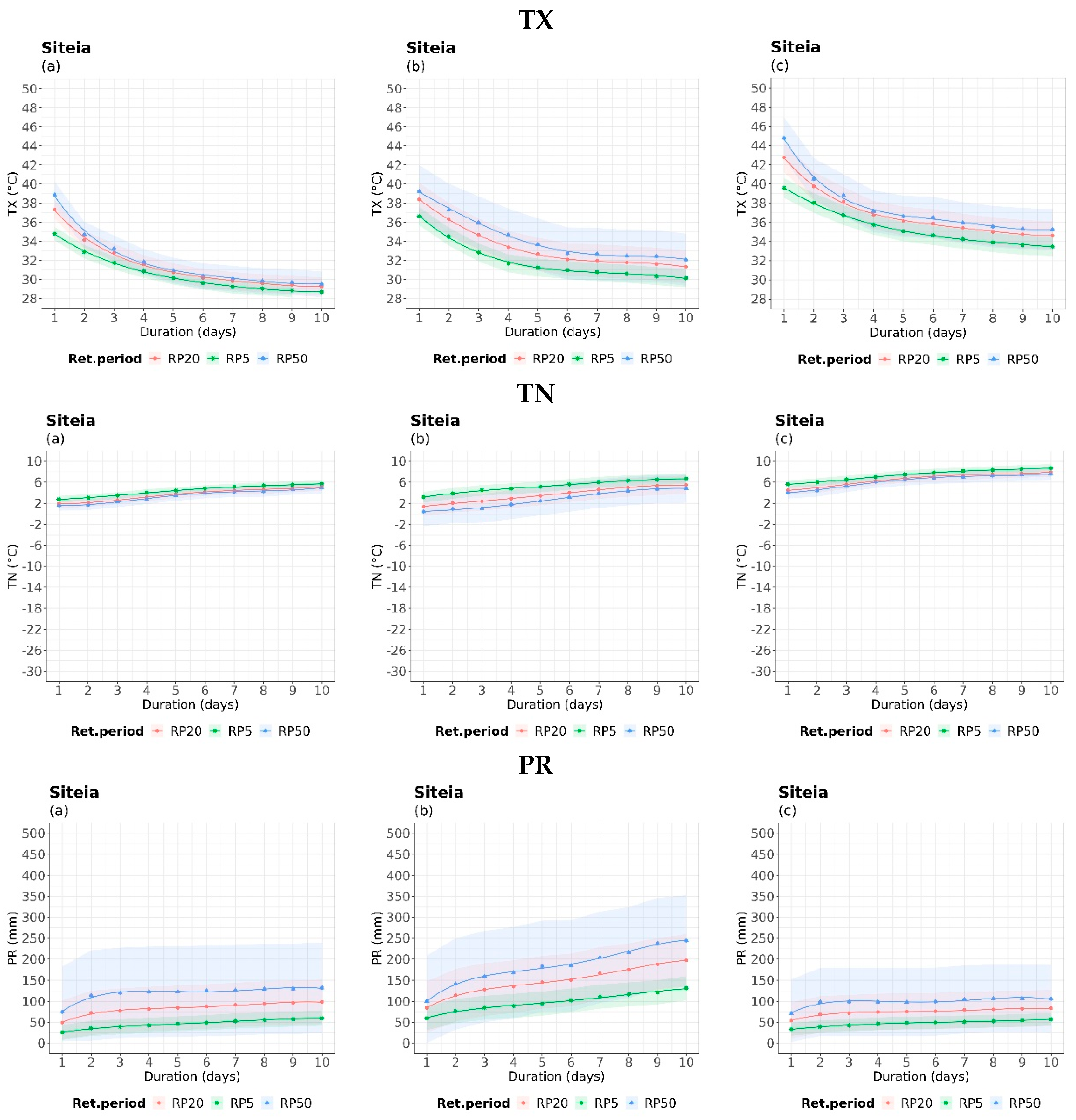
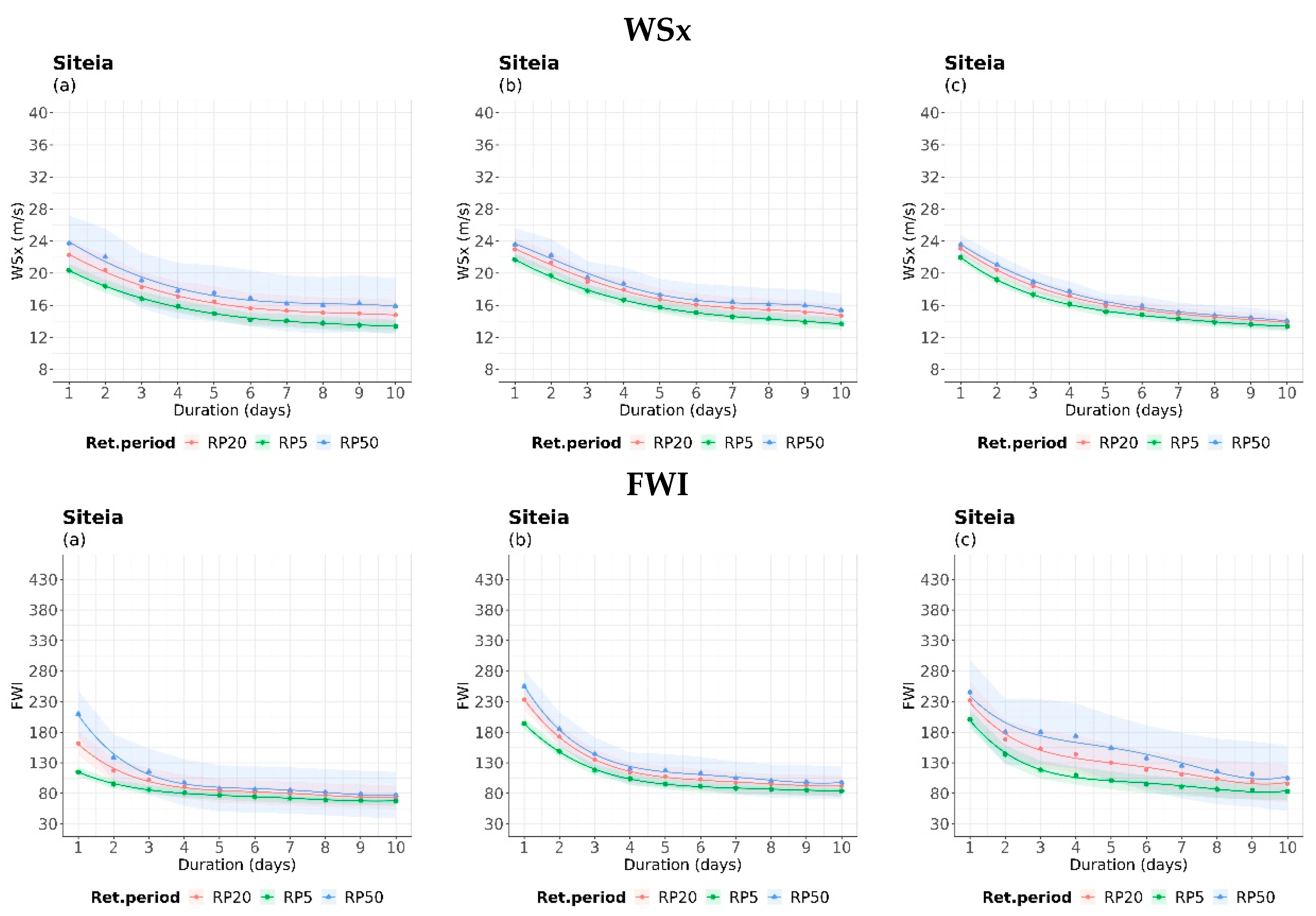
In Section 3.2, we will discuss future risk assessment. To estimate the IDRP curves for future periods, we considered two different time frames: near and far future. The left column of the IDRP curves represents the historical period, while the next two columns represent the near and far future periods. We cannot rely solely on the historical period to assess future risk, as the nature of risk changes over time. Therefore, we applied the same curves to study how extreme events can be affected by climate change. In Figure S5a,c for TX, we can see that the intensity of TX is progressively increasing in the case study of Larissa. For example, an intensity of 40 °C with 5 days of duration in the historical period is expected to change to an intensity of 47 °C with the same duration in the far future period, with a likelihood of a 50-year return period. The confidence intervals (CIs) vary depending on the hazard examined and the historical and future periods. For instance, CIs are larger in the near future period for TN than those in the historical or far future periods, and larger in the far future for FWI in the case study of Alexandroupolis. Due to space limitations, we present only one case study here as a demonstration area of the methodology: Siteia. The corresponding plots of the rest of the case studies can be found in the Supplementary Materials.
The analysis in this work involved studying extreme events and their characteristics in the future, which could be attributed to internal hazard dynamics. The IDRP curves showed different gradients among the historical, near, and future periods concerning the variable and location, thereby showcasing different durations of the extreme values. Changes were also observed in the maximum value of the intensity between the different periods. For instance, in Methoni, the highest-intensity value of FWI in the 50-year IDRP curve lasted for 1 day, whereas in the near-future period, the maximum value persisted for 3 days. Moreover, the maximum intensity values varied from ~120 in the historical period to ~260 in the near future and ~320 in the far-future periods, indicating potential increases in the maximum value of the extreme variable in the future. Similarly, in the case of Siteia, the IDRP curve showed that high-intensity precipitation events lasted no longer than 2–3 days in the historical period, but the intensity and duration increased rapidly in the near future (see Figure 5a,b for PR). To highlight these phenomena, the analysis involved distinct subsections based on the examined variable, aiming to point out the most important results.
3.2. Analysis of Multi-Hazard Scenarios under Climate Change
The discussion was broadened to include a comparative analysis of the IDRP curves related to extreme events between historical and future periods for each variable. Additionally, some general aspects that arose for the three case studies presented here were also explored. Specifically, the impact of climate change on the selected case studies can be summarized as follows:
- There was an increase in the intensity of TX values in both future periods when compared to historical data. However, there was also a reduction in TX values over time, although this resulted in a shift towards prolonged heat that is expected to continue until the end of the 21st century.
- An observable flattening of TX curves for the hottest days suggests highlighting heat waves.
- It was observed that the highest intensity of TX value lasted for 1 day in the far future, with a significant increase compared to the reference period’s 1-day value and a prolonged duration of high TX.
- It was observed that in TN, lower intensities were noticed in large return periods, while a higher intensity was observed in the smallest duration of 1 day. Additionally, TN’s intensity seemed to have lower changes and variability among historical and future periods, as well as among different return periods in terms of IDRP curves. In some cases, TN shifted to higher-intensity values, which implies colder extreme events (lower values of TN) in the near future period.
- Precipitation intensity increased with duration in the near future (mainly under 50-year RP) and decreased in the far future.
- Extreme winds typically lasted no more than 1 day and showed low variability.
- FWI values varied in duration up to 3 days, and the curves for 20- and 50-year RPs differed slightly based on duration.
- (a)
- The case study of Siteia
In the Siteia case study (Figure 5), there was a noticeable increase in TX intensity values in the far future. The behavior of TN’s IDRP curves was similar to that of Kastoria (Figure S3) in the near future, indicating a small increase in cold extreme events of short duration compared to other periods. Additionally, the 20- and 50-year IDRP curves did not vary in the far future compared to the historical period. Regarding rainfall extreme events, the worst-case scenario of a 50-year IDRP curve estimated an extreme rainfall of 125 mm of 3-day duration in the historical period. However, in the far future, there was a progressive increase in intensity and duration of extreme precipitation, yielding 175 mm in 5 days. In the far future, the precipitation’s intensity decreased almost to the levels of the historical period. High-intensity values of maximum winds varied between 20 and 24 m/s, with a duration of 1–2 days during all periods and a reduction in duration. Additionally, there was a shift towards higher WSX values of the 5-year curve in the far future. Regarding fire weather danger, the extreme values of FWI were related to 1-day duration and increased in the historical period in the range of 100–230 to 200–270 in the near and far future periods, respectively.
Figure 5.
Intensity–duration–return period curves of the examined variables for 5-, 20-, and 50-year return periods, during (a) the historical period (1980–2004), (b) near future period (2025–2049), and (c) far future (2075–2099) for Siteia. The colored areas illustrate the 99% confidence intervals for each return period.
3.3. Maximum and Minimum Temperature
In this section, we discuss the impact of IDRP curves on extreme temperatures in specific locations, as shown in Figure 6 for TX and Figure 7 for TN.
In Alexandroupolis, we observed an increase in both future periods and intensity estimates, indicating progressively hotter temperatures in the far future. We also noticed that the curvature of all IDRP curves flattened in the historical period after a 7-day duration and changed compared to the near future, indicating more persisting high temperatures. Additionally, the difference among the different return period curves amplified in the future. In the case of Larissa, the increase in the intensity values of TX was the highest among the other locations in both future periods. Please note that the range of TX values goes up to 60 °C on the y-axis. The Larissa location showed the highest intensity (1-day duration) of around 50 °C and the most prolonged heat (up to 10 days) in the far future with at least 41 °C (in 5-year RP) and 45 °C (in 50-year RP). Moreover, an interesting exception is that of Methoni, where the intensity of extreme heat of rare events (1 day) reduced in the far future (lower than 44 °C) compared to the near future in what concerns the 100-year RP. In addition, intensity values were amplified among the different IDRP curves in the near future.
In Naxos, we observed the most intense events based on the 20- and 50-year IDRP curves for a duration of 1 day. Similarly, a higher intensity in Siteia was also observed for 1 day, but the IDRP curves flattened rapidly compared to other locations.
When it comes to the extremes TN, all case studies revealed a projected increase of cold spells in the near future in various locations such as Alexandroupolis, Corfu, Kastoria, Naxos, Methoni, Larissa, Elliniko, and Siteia. This would result in colder conditions, as shown in Figure 7 for Elliniko and Kastoria. However, in the far future, a shift to warmer values was observed compared to the historical and near-future periods, especially when observing the IDRP curve of a 50-year return period. In the far future, the representation of 20- and 50-year IDRP curves showed an almost identical performance. The thinner ranges of Cis observed in the far future in Figure 7 could imply that a notable increase in minimum temperature is highly likely. This is because narrow Cis imply low variability of the estimated annual maximum values of the examined hazard [71].
3.4. Wind Speed
It was observed that in all IDRP (intensity–duration–return period) curves, there was no significant variation of wind speed after a duration of 5–6 days. The curves became almost flat and, in some areas, the 20- and 50-year IDRP curves yielded similar intensities of extreme winds with small deviations. In the near future, a small increase in the intensity of wind speed is projected in Corfu and Naxos (Figures S2b and S7b, included in the Supplementary Materials), while in Alexandroupolis (Figure 8c), the winds are projected to progressively reduce compared to the historical period. For the three examined return periods, high-intensity values of extreme winds are estimated to last mostly up to 1 day, with a few exceptions. For instance, Alexandroupolis in the far future is projected to have 2 days of high-intensity wind speed in the 50-year IDRP curve. The intensity of extreme winds on the 50-year IDRP curve decreases after a duration of 7 days. It was also observed that there is a geographical dependence of areas (Figure 8). For example, higher-intensity wind speed was estimated in Alexandroupolis than in Elliniko. No notable discrepancies were found among the 20- and 50-year IDRP curves in the case of the latter. Furthermore, larger values of the estimated confidence intervals were observed in the case study of Alexandroupolis than in Elliniko. This could be attributed to the sampling variability of the first area.
3.5. Precipitation
Several areas, as depicted in Figure 9, are projected to experience a significant increase in precipitation in the near future, with variations among the three different return periods (Corfu, Kastoria, Elliniko, Alexandroupolis, Methoni, Siteia). This increase is justified by the changing seasonal and annual precipitation patterns observed in these areas discussed in Politi et al.’s 2022 study [54]. However, all areas are projected to experience a reduction in precipitation in the far future. For instance, in Siteia, the intensity value for a 2-day duration is estimated to be around 140 mm in the near future, while it is expected to decrease to about 100 mm in the far future. Furthermore, the historical data show that the highest amount of precipitation is expected to fall within a duration of 2 to 4 days. In the case of Alexandroupolis, more extreme rain events are predicted to occur in the far future but with shorter durations compared to the near future period. The IDRP curves of Alexandroupolis in the near future seem to stabilize after 4 days, while those of Methoni and Siteia show an increasing trend. In the near future, Kastoria is expected to experience extreme precipitation of 160 mm within 3 days, based on the 50-year IDRP curve and 110 mm for the 20-year IDRP curve. These amounts will notably decrease in the far future. In general, the estimated confidence intervals (Cis) also vary in different time periods and areas.
3.6. Fire Weather Index
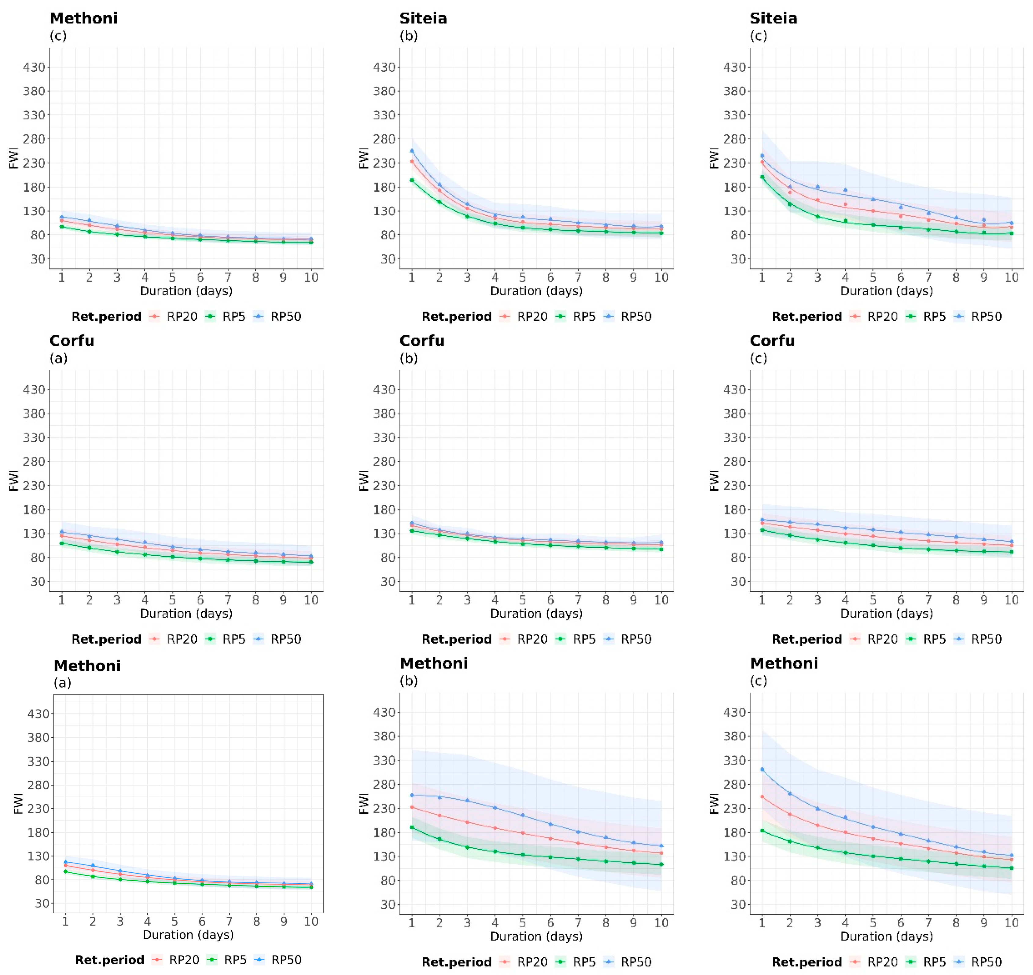
It is interesting to note that in the case of Siteia, while the highest FWI intensity values were obtained with a 1-day duration in the historical and near future periods (Figure 10a,b), the situation changed in considering the far future, particularly in the 50-year IDRP curve. This curve shows a persisting duration of 4 days with higher FWI values (180). A similar trend is observed in the case of Corfu, where there is an increase in the duration of extreme fire weather in the far future. Additionally, there is a notable increase in intensity (change of more than 100 units of FWI intensity values) and duration in Methoni for both future periods, along with large Cis in both periods.
4. Conclusions
The purpose of this work was to introduce an advanced and comprehensible methodology that can be used to evaluate the risk occurrences of different extreme events in both historical and future periods. The approach was designed to create IDRP curves that can assess multi-hazard scenarios associated with various climate hazards such as heat waves, cold waves, wildfires, extreme precipitation, and wind. The methodology considered the three most significant characteristics of these hazards: intensity, duration, and return periods. These characteristics are commonly used to describe and characterize extreme events that may vary across spatial and temporal scales.
The proposed approach can be practically applied to one or multiple geographic locations or regions that have diverse climate conditions. This approach can help assess their vulnerability to climate change by studying the behavior of extreme events. The IDPR curves can represent extreme scenarios, and the respective extreme event can be assessed by its persistence. Additionally, it can be quantified by how extreme it could potentially be.
The analysis showed how IDRP curves can change over time and space, leading to different interpretations of extreme events under a changing climate in Greece. For instance, in the case of the fire weather index (FWI) in Siteia, the curves amplified in the far future, indicating prolonged and more intense fire weather danger conditions. Moreover, the curves’ behavior varied depending on the hazard represented, as deduced from the comparison between minimum temperature (TN) and maximum precipitation (PR) in all cases studied. Additionally, the diversity in the IDPR curves’ behavior, which varied significantly among historical and future periods, in some variables due to climate change, such as the increase of extreme precipitation with longer duration in the near future, indicates the effect of internal hazard dynamics.
The significance of this work lies in its multidimensional approach, which is based on the IDRP curves. It takes into account not only historical information but also future climate risks for the first time. The proposed multi-hazard extreme scenario methodology can be applied to any geographic area or region, provided that continuous and reliable climate datasets are available. We have not identified any potential barriers to the presented approach. According to the World Meteorological Organization (WMO) [72], different countries have adopted different theoretical distributions as standard models for flood and/or rainfall frequency analysis. Therefore, the selection of the best-fitted theoretical distributions in extreme values should be primarily examined depending on the variable and location [44]. Further analysis of the extremes in terms of distributions could be applied by considering multivariate distributions in future investigations, as in [73]. Moreover, future investigations could involve the consideration of compounding among multiple hazards. The applied methodology could be expanded not only spatially but also to include several indices related to socioeconomic sectors, water and energy resource management, and tourism. These sectors would be severely impacted by severe extreme climate hazards, affecting the exposed populations directly and/or indirectly.
In conclusion, the above methodology can provide an estimation of potential extreme events that may arise from different climate variables, based on the quantification of intensity, duration, and return period characteristics. This estimation can be made in the context of different climate change scenarios and for a certain area. By considering these characteristics, we can configure the risk level and understand how it may change in the future. This information can be used to obtain more comprehensive estimates that can be considered by civil protection, policy makers, and relevant stakeholders in the design of risk reduction and preparedness plans. Therefore, the estimation of extreme events based on the quantification of different multi-hazard scenarios can offer a more complete overview of the future risk. This can help in designing and reconsidering adaptation strategies for the development and implementation of effective policies towards more sustainable and resilient societies and ecosystems.
Supplementary Materials
The following supporting information can be downloaded at: https://www.mdpi.com/article/10.3390/cli11120242/s1, Figure S1: Case study of Alexandroupolis; Figure S2: Case study of Corfu; Figure S3: Case study of Kastoria; Figure S4: Case study of Elliniko; Figure S5: Case study of Larissa; Figure S6: Case study of Methoni; Figure S7: Case study of Naxos.
Author Contributions
Conceptualization, A.S. and D.V.; methodology, A.S.; software, N.P.; validation, A.S., N.P. and D.V.; formal analysis, N.P.; investigation, A.S. and N.P.; data curation, N.P.; writing—original draft preparation, A.S. and N.P.; writing—review and editing, A.S. and D.V.; visualization, N.P.; supervision, A.S. and D.V. All authors have read and agreed to the published version of the manuscript.
Funding
This work has received partial funding from the Horizon Europe Framework Programme (HORIZON) Research and Innovation Actions under grant agreement No 101074004 (C2IPMRESS).
Data Availability Statement
The data presented in this study are available on request from the corresponding author.
Acknowledgments
This work was supported by computational time granted from the Greek Research and Technology Network (GRNET) in the National HPC facility, ARIS, under projects ID HRCOG (pr004020) and HRPOG (pr006028).
Conflicts of Interest
The authors declare no conflict of interest.
References
- Poljanšek, K.; Casajus Valles, A.; Marín Ferrer, M.; De Jager, A.; Dottori, F.; Galbusera, L.; García Puerta, B.; Giannopoulos, G.; Girgin, S.; Hernandez Ceballos, M.; et al. Recommendations for National Risk Assessment for Disaster Risk Management in EU; Publications Office of the European Union: Luxembourg, 2019; ISBN 978-92-79-98366-5. [Google Scholar]
- UNISDR. National Disaster Risk Assessment Words into Action Guidelines Governance System, Methodologies, and Use of Results; The United Nations Office for Disaster Risk Reduction: Geneva, Switzerland, 2017. [Google Scholar]
- IAEA; Boyce, T.; Courtin, E. Deterministic Safety Analysis for Nuclear Power Plants; IAEA Safety Standards Series No. SSG-2; International Atomic Energy Agency: Vienna, Austria, 2010; Volume SSG-2, ISBN 9201107064. [Google Scholar]
- EUROCODES EN 1991-1-4; Eurocode 1: Actions on Structures—Part 1–4: General Actions—Wind Actions. CEN: Brussels, Belgium, 2005.
- François, B.; Schlef, K.E.; Wi, S.; Brown, C.M. Design Considerations for Riverine Floods in a Changing Climate—A Review. J. Hydrol. 2019, 574, 557–573. [Google Scholar] [CrossRef]
- World Meteorological Organization. Guidelines on the Defintion and Characterization of Extreme Weather and Climate Events; WMO: Geneva, Switzerland, 2023; 27p. [Google Scholar]
- IPCC-AR6. Weather and Climate Extreme Events in a Changing Climate. In Climate Change 2021—The Physical Science Basis; Cambridge University Press: Cambridge, UK, 2023; pp. 1513–1766. [Google Scholar]
- Vogel, M.M.; Hauser, M.; Seneviratne, S.I. Projected Changes in Hot, Dry and Wet Extreme Events’ Clusters in CMIP6 Multi-Model Ensemble. Environ. Res. Lett. 2020, 15, 094021. [Google Scholar] [CrossRef]
- Liu, K.; Harrison, M.T.; Yan, H.; Liu, D.L.; Meinke, H.; Hoogenboom, G.; Wang, B.; Peng, B.; Guan, K.; Jaegermeyr, J.; et al. Silver Lining to a Climate Crisis in Multiple Prospects for Alleviating Crop Waterlogging under Future Climates. Nat. Commun. 2023, 14, 765. [Google Scholar] [CrossRef]
- Li, L.; Wang, B.; Feng, P.; Jägermeyr, J.; Asseng, S.; Müller, C.; Macadam, I.; Liu, D.L.; Waters, C.; Zhang, Y.; et al. The Optimization of Model Ensemble Composition and Size Can Enhance the Robustness of Crop Yield Projections. Commun. Earth Commun. Earth Environ. 2023, 4, 362. [Google Scholar] [CrossRef]
- Ouarda, T.B.M.J.; Charron, C. Changes in the Distribution of Hydro-Climatic Extremes in a Non-Stationary Framework. Sci. Rep. 2019, 9, 8104. [Google Scholar] [CrossRef]
- Slater, L.J.; Anderson, B.; Buechel, M.; Dadson, S.; Han, S.; Harrigan, S.; Kelder, T.; Kowal, K.; Lees, T.; Matthews, T.; et al. Nonstationary Weather and Water Extremes: A Review of Methods for Their Detection, Attribution, and Management. Hydrol. Earth Syst. Sci. 2021, 25, 3897–3935. [Google Scholar] [CrossRef]
- Hamdi, Y.; Duluc, C.-M.; Rebour, V. Temperature Extremes: Estimation of Non-Stationary Return Levels and Associated Uncertainties. Atmosphere 2018, 9, 129. [Google Scholar] [CrossRef]
- Findell, K.L.; Berg, A.; Gentine, P.; Krasting, J.P.; Lintner, B.R.; Malyshev, S.; Santanello, J.A.; Shevliakova, E. The Impact of Anthropogenic Land Use and Land Cover Change on Regional Climate Extremes. Nat. Commun. 2017, 8, 989. [Google Scholar] [CrossRef]
- Li, L.; Zha, Y.; Zhang, J. Spatially Non-Stationary Effect of Underlying Driving Factors on Surface Urban Heat Islands in Global Major Cities. Int. J. Appl. Earth Obs. Geoinf. 2020, 90, 102131. [Google Scholar] [CrossRef]
- Schlef, K.E.; Kunkel, K.E.; Brown, C.; Demissie, Y.; Lettenmaier, D.P.; Wagner, A.; Wigmosta, M.S.; Karl, T.R.; Easterling, D.R.; Wang, K.J.; et al. Incorporating Non-Stationarity from Climate Change into Rainfall Frequency and Intensity-Duration-Frequency (IDF) Curves. J. Hydrol. 2023, 616, 128757. [Google Scholar] [CrossRef]
- Fadhel, S.; Rico-Ramirez, M.A.; Han, D. Uncertainty of Intensity–Duration–Frequency (IDF) Curves Due to Varied Climate Baseline Periods. J. Hydrol. 2017, 547, 600–612. [Google Scholar] [CrossRef]
- Clausen, B.; Pearson, C.P. Regional Frequency Analysis of Annual Maximum Streamflow Drought. J. Hydrol. 1995, 173, 111–130. [Google Scholar] [CrossRef]
- Baran-Gurgul, K. A Comparison of Three Parameter Estimation Methods of the Gamma Distribution of Annual Maximum Low Flow Duration and Deficit in the Upper Vistula Catchment (Poland). ITM Web Conf. 2018, 23, 00001. [Google Scholar] [CrossRef]
- Tosunoglu, F.; Kisi, O. Joint Modelling of Annual Maximum Drought Severity and Corresponding Duration. J. Hydrol. 2016, 543, 406–422. [Google Scholar] [CrossRef]
- AghaKouchak, A.; Cheng, L.; Mazdiyasni, O.; Farahmand, A. Global Warming and Changes in Risk of Concurrent Climate Extremes: Insights from the 2014 California Drought. Geophys. Res. Lett. 2014, 41, 8847–8852. [Google Scholar] [CrossRef]
- Slater, L.; Villarini, G.; Archfield, S.; Faulkner, D.; Lamb, R.; Khouakhi, A.; Yin, J. Global Changes in 20-Year, 50-Year, and 100-Year River Floods. Geophys. Res. Lett. 2021, 48, e2020GL091824. [Google Scholar] [CrossRef]
- Gu, L.; Yin, J.; Gentine, P.; Wang, H.-M.; Slater, L.J.; Sullivan, S.C.; Chen, J.; Zscheischler, J.; Guo, S. Large Anomalies in Future Extreme Precipitation Sensitivity Driven by Atmospheric Dynamics. Nat. Commun. 2023, 14, 3197. [Google Scholar] [CrossRef] [PubMed]
- Gu, X.; Ye, L.; Xin, Q.; Zhang, C.; Zeng, F.; Nerantzaki, S.D.; Papalexiou, S.M. Extreme Precipitation in China: A Review on Statistical Methods and Applications. Adv. Water Resour. 2022, 163, 104144. [Google Scholar] [CrossRef]
- Nerantzaki, S.D.; Papalexiou, S.M. Assessing Extremes in Hydroclimatology: A Review on Probabilistic Methods. J. Hydrol. 2022, 605, 127302. [Google Scholar] [CrossRef]
- Wasko, C.; Westra, S.; Nathan, R.; Orr, H.G.; Villarini, G.; Villalobos Herrera, R.; Fowler, H.J. Incorporating Climate Change in Flood Estimation Guidance. Philos. Trans. R. Soc. A Math. Phys. Eng. Sci. 2021, 379, 20190548. [Google Scholar] [CrossRef]
- Martel, J.-L.; Brissette, F.P.; Lucas-Picher, P.; Troin, M.; Arsenault, R. Climate Change and Rainfall Intensity–Duration–Frequency Curves: Overview of Science and Guidelines for Adaptation. J. Hydrol. Eng. 2021, 26, 03121001. [Google Scholar] [CrossRef]
- Salas, J.D.; Obeysekera, J.; Vogel, R.M. Techniques for Assessing Water Infrastructure for Nonstationary Extreme Events: A Review. Hydrol. Sci. J. 2018, 63, 325–352. [Google Scholar] [CrossRef]
- Yan, L.; Xiong, L.; Jiang, C.; Zhang, M.; Wang, D.; Xu, C.-Y. Updating Intensity–Duration–Frequency Curves for Urban Infrastructure Design under a Changing Environment. Wires Water 2021, 8, e1519. [Google Scholar] [CrossRef]
- Young, A.F.; Jorge Papini, J.A. How Can Scenarios on Flood Disaster Risk Support Urban Response? A Case Study in Campinas Metropolitan Area (São Paulo, Brazil). Sustain. Cities Soc. 2020, 61, 102253. [Google Scholar] [CrossRef]
- Eilander, D.; Couasnon, A.; Sperna Weiland, F.C.; Ligtvoet, W.; Bouwman, A.; Winsemius, H.C.; Ward, P.J. Modeling Compound Flood Risk and Risk Reduction Using a Globally Applicable Framework: A Pilot in the Sofala Province of Mozambique. Nat. Hazards Earth Syst. Sci. 2023, 23, 2251–2272. [Google Scholar] [CrossRef]
- Couasnon, A.; Scussolini, P.; Tran, T.V.T.; Eilander, D.; Muis, S.; Wang, H.; Keesom, J.; Dullaart, J.; Xuan, Y.; Nguyen, H.Q.; et al. A Flood Risk Framework Capturing the Seasonality of and Dependence Between Rainfall and Sea Levels—An Application to Ho Chi Minh City, Vietnam. Water Resour. Res. 2022, 58, e2021WR030002. [Google Scholar] [CrossRef]
- Bates, P.D.; Quinn, N.; Sampson, C.; Smith, A.; Wing, O.; Sosa, J.; Savage, J.; Olcese, G.; Neal, J.; Schumann, G.; et al. Combined Modeling of US Fluvial, Pluvial, and Coastal Flood Hazard under Current and Future Climates. Water Resour. Res. 2021, 57, e2020WR028673. [Google Scholar] [CrossRef]
- Shin, J.-Y.; Kim, K.R.; Ha, J.-C. Intensity-Duration-Frequency Relationship of WBGT Extremes Using Regional Frequency Analysis in South Korea. Environ. Res. 2020, 190, 109964. [Google Scholar] [CrossRef]
- Mazdiyasni, O.; Sadegh, M.; Chiang, F.; AghaKouchak, A. Heat Wave Intensity Duration Frequency Curve: A Multivariate Approach for Hazard and Attribution Analysis. Sci. Rep. 2019, 9, 14117. [Google Scholar] [CrossRef]
- Brown, S.J. Future Changes in Heatwave Severity, Duration and Frequency Due to Climate Change for the Most Populous Cities. Weather Clim. Extrem. 2020, 30, 100278. [Google Scholar] [CrossRef]
- Ben Alaya, M.A.; Zwiers, F.W.; Zhang, X. On Estimating Long Period Wind Speed Return Levels from Annual Maxima. Weather Clim. Extrem. 2021, 34, 100388. [Google Scholar] [CrossRef]
- Founda, D.; Varotsos, K.V.; Pierros, F.; Giannakopoulos, C. Observed and Projected Shifts in Hot Extremes’ Season in the Eastern Mediterranean. Glob. Planet. Chang. 2019, 175, 190–200. [Google Scholar] [CrossRef]
- Rovithakis, A.; Grillakis, M.G.; Seiradakis, K.D.; Giannakopoulos, C.; Karali, A.; Field, R.; Lazaridis, M.; Voulgarakis, A. Future Climate Change Impact on Wildfire Danger over the Mediterranean: The Case of Greece. Environ. Res. Lett. 2022, 17, 045022. [Google Scholar] [CrossRef]
- Lionello, P.; Scarascia, L. The Relation of Climate Extremes with Global Warming in the Mediterranean Region and Its North Versus South Contrast. Reg. Environ. Chang. 2020, 20, 31. [Google Scholar] [CrossRef]
- Zittis, G.; Hadjinicolaou, P.; Fnais, M.; Lelieveld, J. Projected Changes in Heat Wave Characteristics in the Eastern Mediterranean and the Middle East. Reg. Environ. Chang. 2016, 16, 1863–1876. [Google Scholar] [CrossRef]
- Papaioannou, G.; Efstratiadis, A.; Vasiliades, L.; Loukas, A.; Papalexiou, S.M.; Koukouvinos, A.; Tsoukalas, I.; Kossieris, P. An Operational Method for Flood Directive Implementation in Ungauged Urban Areas. Hydrology 2018, 5, 24. [Google Scholar] [CrossRef]
- Tsaples, G.; Grau, J.M.S.; Aifadopoulou, G.; Tzenos, P. A Simulation Model for the Analysis of the Consequences of Extreme Weather Conditions to the Traffic Status of the City of Thessaloniki, Greece. In Springer Optimization and Its Applications; Springer: Berlin/Heidelberg, Germany, 2021; pp. 259–272. [Google Scholar]
- Vangelis, H.; Zotou, I.; Kourtis, I.M.; Bellos, V.; Tsihrintzis, V.A. Relationship of Rainfall and Flood Return Periods through Hydrologic and Hydraulic Modeling. Water 2022, 14, 3618. [Google Scholar] [CrossRef]
- Galiatsatou, P.; Iliadis, C. Intensity-Duration-Frequency Curves at Ungauged Sites in a Changing Climate for Sustainable Stormwater Networks. Sustainability 2022, 14, 1229. [Google Scholar] [CrossRef]
- van der Schriek, T.; Varotsos, K.V.; Giannakopoulos, C.; Founda, D. Projected Future Temporal Trends of Two Different Urban Heat Islands in Athens (Greece) under Three Climate Change Scenarios: A Statistical Approach. Atmosphere 2020, 11, 637. [Google Scholar] [CrossRef]
- Vlachogiannis, D.; Sfetsos, A.; Markantonis, I.; Politi, N.; Karozis, S.; Gounaris, N. Quantifying the Occurrence of Multi-Hazards Due to Climate Change. Appl. Sci. 2022, 12, 1218. [Google Scholar] [CrossRef]
- Gill, J.C.; Malamud, B.D. Hazard Interactions and Interaction Networks (Cascades) within Multi-Hazard. Earth Syst. Dyn. 2016, 7, 659–679. [Google Scholar] [CrossRef]
- Gill, J.C.; Malamud, B.D. Reviewing and Visualizing the Interactions of Natural Hazards. Rev. Geophys. 2014, 52, 680–722. [Google Scholar] [CrossRef]
- Li, S.H. Design Wind Speed for Buildings and Facilities with Non-Standard Design Life in Canadian Wind Climates. Front. Built Environ. 2022, 8, 829533. [Google Scholar] [CrossRef]
- Riahi, K.; Rao, S.; Krey, V.; Cho, C.; Chirkov, V.; Fischer, G.; Kindermann, G.; Nakicenovic, N.; Rafaj, P. RCP 8.5-A Scenario of Comparatively High Greenhouse Gas Emissions. Clim. Chang. 2011, 109, 33–57. [Google Scholar] [CrossRef]
- Van Wagner, C.E.; Pickett, T.L. Equations and FORTRAN Program for the Canadian Forest Fire Weather Index System; Forestry Technical Report 33; Canadian Forestry Service, Petawawa National Forestry Institute: Chalk River, ON, Canada, 1985; 18p. [Google Scholar]
- Hoskingt, J.R.M. L-Moments: Analysis and Estimation of Distributions Using Linear Combinations of Order Statistics. J. R. Stat. Soc. Ser. B Stat. Methodol. 1990, 52, 105–124. [Google Scholar]
- Feng Huang, Y.; Mirzaei, M.; Zaki, M.; Amin, M. ScienceDirect Uncertainty Quantification in Rainfall Intensity Duration Frequency Curves Based on Historical Extreme Precipitation Quantiles. Procedia Eng. 2016, 154, 426–432. [Google Scholar] [CrossRef]
- Yeo, M.-H.; Nguyen, V.-T.-V.; Kpodonu, T.A. Characterizing Extreme Rainfalls and Constructing Confidence Intervals for IDF Curves Using Scaling-GEV Distribution Model. Int. J. Climatol. 2021, 41, 456–468. [Google Scholar] [CrossRef]
- Kharin, V.V.; Zwiers, F.W. Estimating Extremes in Transient Climate Change Simulations. J. Clim. 2005, 18, 1156–1173. [Google Scholar] [CrossRef]
- Skamarock, W.C.; Skamarock, W.C.; Klemp, J.B.; Dudhia, J.; Gill, D.O.; Barker, D.M.; Wang, W.; Powers, J.G. A Description of the Advanced Research WRF Version 3. NCAR Tech. Note 2008, 475, 113. [Google Scholar]
- Hazeleger, W.; Severijns, C.; Semmler, T.; Ştefǎnescu, S.; Yang, S.; Wang, X.; Wyser, K.; Dutra, E.; Baldasano, J.M.; Bintanja, R.; et al. EC-Earth: A Seamless Earth-System Prediction Approach in Action. Bull. Am. Meteorol. Soc. 2010, 91, 1357–1364. [Google Scholar] [CrossRef]
- Hazeleger, W.; Wang, X.; Severijns, C.; Ştefănescu, S.; Bintanja, R.; Sterl, A.; Wyser, K.; Semmler, T.; Yang, S.; van den Hurk, B.; et al. EC-Earth V2.2: Description and Validation of a New Seamless Earth System Prediction Model. Clim. Dyn. 2012, 39, 2611–2629. [Google Scholar] [CrossRef]
- Hong, S.-Y.; Lim, J.-O. The WRF Single-Moment 6-Class Microphysics Scheme (WSM6). J. Korean Meteor. Soc. 2006, 42, 129–151. [Google Scholar]
- Iacono, M.J.; Delamere, J.S.; Mlawer, E.J.; Shephard, M.W.; Clough, S.A.; Collins, W.D. Radiative Forcing by Long-Lived Greenhouse Gases: Calculations with the AER Radiative Transfer Models. J. Geophys. Res. 2008, 113, D13103. [Google Scholar] [CrossRef]
- Janjić, Z.I. Nonsingular Implementation of the Mellor-Yamada Level 2.5 Scheme in the NCEP Meso Model; Technical Report, National Centers for Environmental Prediction (NCEP), Office Note No. 437; 2001; 61p. Available online: https://repository.library.noaa.gov/view/noaa/11409 (accessed on 13 November 2023).
- Mellor, G.L.; Yamada, T. Development of a Turbulence Closure Model for Geophysical Fluid Problems. Rev. Geophys. 1982, 20, 851. [Google Scholar] [CrossRef]
- Betts, A.K.; Miller, M.J. A New Convective Adjustment Scheme. Part II: Single Column Tests Using GATE Wave, BOMEX, ATEX and Arctic Air-Mass Data Sets. Q. J. R. Meteorol. Soc. 1986, 112, 693–709. [Google Scholar] [CrossRef]
- Chen, F.; Dudhia, J.; Chen, F.; Dudhia, J. Coupling an Advanced Land Surface–Hydrology Model with the Penn State–NCAR MM5 Modeling System. Part I: Model Implementation and Sensitivity. Mon. Weather Rev. 2001, 129, 569–585. [Google Scholar] [CrossRef]
- Politi, N.; Vlachogiannis, D.; Sfetsos, A.; Nastos, P.T. High-Resolution Dynamical Downscaling of ERA-Interim Temperature and Precipitation Using WRF Model for Greece. Clim. Dyn. 2021, 57, 799–825. [Google Scholar] [CrossRef]
- Politi, N.; Vlachogiannis, D.; Sfetsos, A.; Nastos, P.T. High Resolution Projections for Extreme Temperatures and Precipitation over Greece. Clim. Dyn. 2022, 61, 633–667. [Google Scholar] [CrossRef]
- Katopodis, T.; Markantonis, I.; Vlachogiannis, D.; Politi, N.; Sfetsos, A. Assessing Climate Change Impacts on Wind Characteristics in Greece through High Resolution Regional Climate Modelling. Renew. Energy 2021, 179, 427–444. [Google Scholar] [CrossRef]
- Katopodis, T.; Vlachogiannis, D.; Politi, N.; Gounaris, N.; Karozis, S.; Sfetsos, A. Assessment of Climate Change Impacts on Wind Resource Characteristics and Wind Energy Potential in Greece. J. Renew. Sustain. Energy 2019, 11, 066502. [Google Scholar] [CrossRef]
- Kim, J.-Y.; So, B.-J.; Kwon, H.-H.; Kim, T.-W.; Lee, J.-H. Estimation of Return Period and Its Uncertainty for the Recent 2013–2015 Drought in the Han River Watershed in South Korea. Hydrol. Res. 2018, 49, 1313–1329. [Google Scholar] [CrossRef]
- Yeo, M.-H.; Nguyen, V.-T.-V.; Kim, Y.S.; Kpodonu, T.A. An Integrated Extreme Rainfall Modeling Tool (SDExtreme) for Climate Change Impacts and Adaptation. Water Resour. Manag. 2022, 36, 3153–3179. [Google Scholar] [CrossRef]
- Statistical Distributions for Flood Frequency Analysis | World Meteorological Organization. Available online: https://community.wmo.int/en/bookstore/statistical-distributions-flood-frequency-analysis (accessed on 5 December 2023).
- Baran-Gurgul, K. The Risk of Extreme Streamflow Drought in the Polish Carpathians & mdash; A Two-Dimensional Approach. Int. J. Environ. Res. Public Health 2022, 19, 14095. [Google Scholar] [CrossRef] [PubMed]
Figure 1.
Conceptual workflow for the representation of extreme hazard scenarios.

Figure 2.
Locations of the nearest grid point to the studied weather stations with elevation.

Figure 3.
Modeling domains: d01 refers to the outermost domain of 20 km and d02 to the nested domain of 5 km (region of Greece).
Figure 3.
Modeling domains: d01 refers to the outermost domain of 20 km and d02 to the nested domain of 5 km (region of Greece).

Figure 4.
Historical estimates of intensity–duration–return period curves of the examined variables (a) TX, (b) TN, (c) PR, (d) WSx, (e) FWI, and (f) snow for 5-, 20-, and 50-year return periods, for Kastoria. The colored areas illustrate the 99% confidence intervals for each return period.
Figure 4.
Historical estimates of intensity–duration–return period curves of the examined variables (a) TX, (b) TN, (c) PR, (d) WSx, (e) FWI, and (f) snow for 5-, 20-, and 50-year return periods, for Kastoria. The colored areas illustrate the 99% confidence intervals for each return period.

Figure 6.
IDRP curves of TX for 5-, 20-, and 50-year return periods, during (a) the historical period (1980–2004), (b) near future period (2025–2049), and (c) far future (2075–2099) for indicative locations. The colored areas illustrate the 99% confidence intervals for each return period.
Figure 6.
IDRP curves of TX for 5-, 20-, and 50-year return periods, during (a) the historical period (1980–2004), (b) near future period (2025–2049), and (c) far future (2075–2099) for indicative locations. The colored areas illustrate the 99% confidence intervals for each return period.
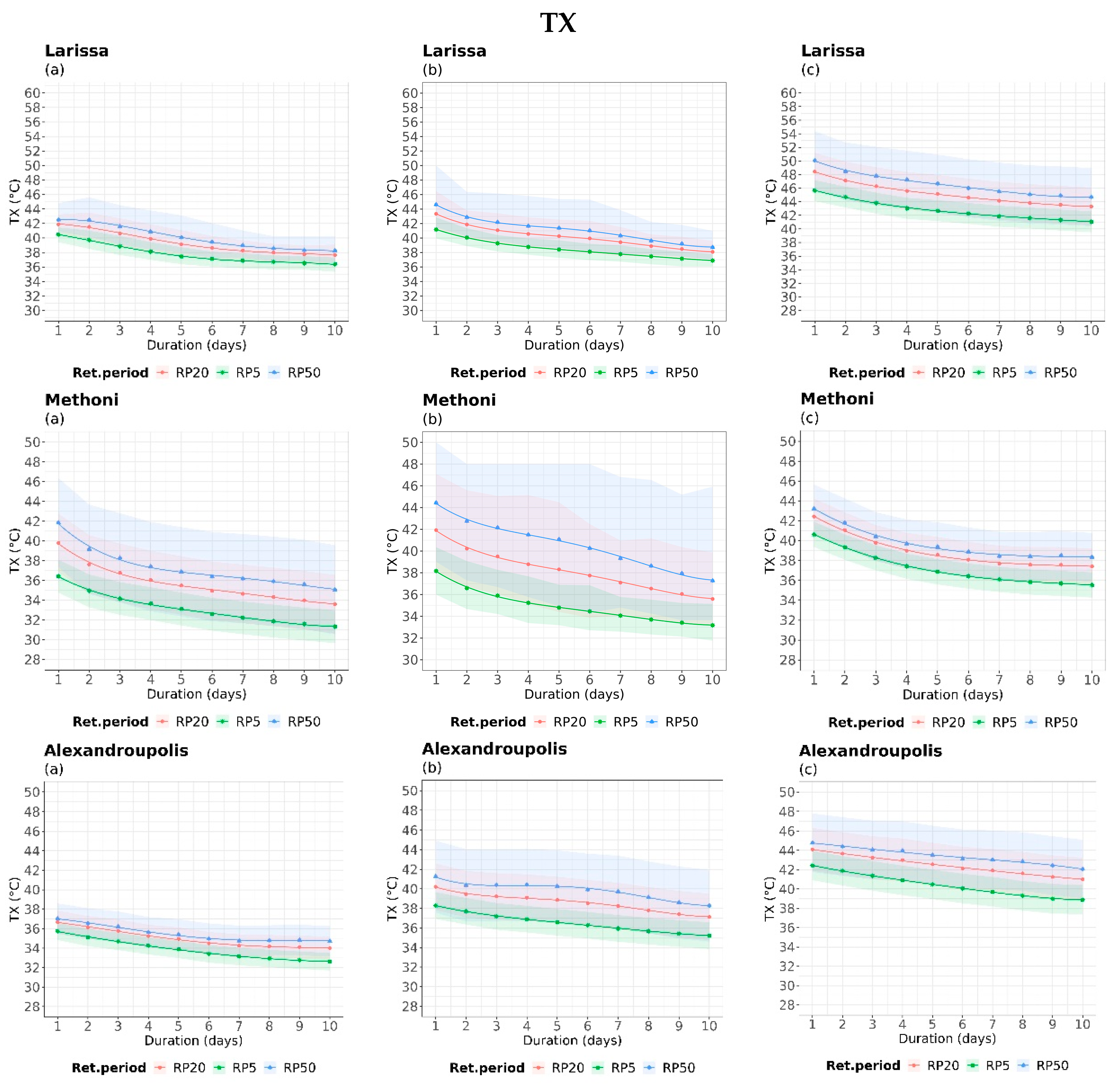
Figure 7.
IDRP curves of TN for 5-, 20-, and 50-year return periods, during (a) the historical period (1980–2004), (b) near future period (2025–2049), and (c) far future (2075–2099) for indicative locations. The colored areas illustrate the 99% confidence intervals for each return period.
Figure 7.
IDRP curves of TN for 5-, 20-, and 50-year return periods, during (a) the historical period (1980–2004), (b) near future period (2025–2049), and (c) far future (2075–2099) for indicative locations. The colored areas illustrate the 99% confidence intervals for each return period.
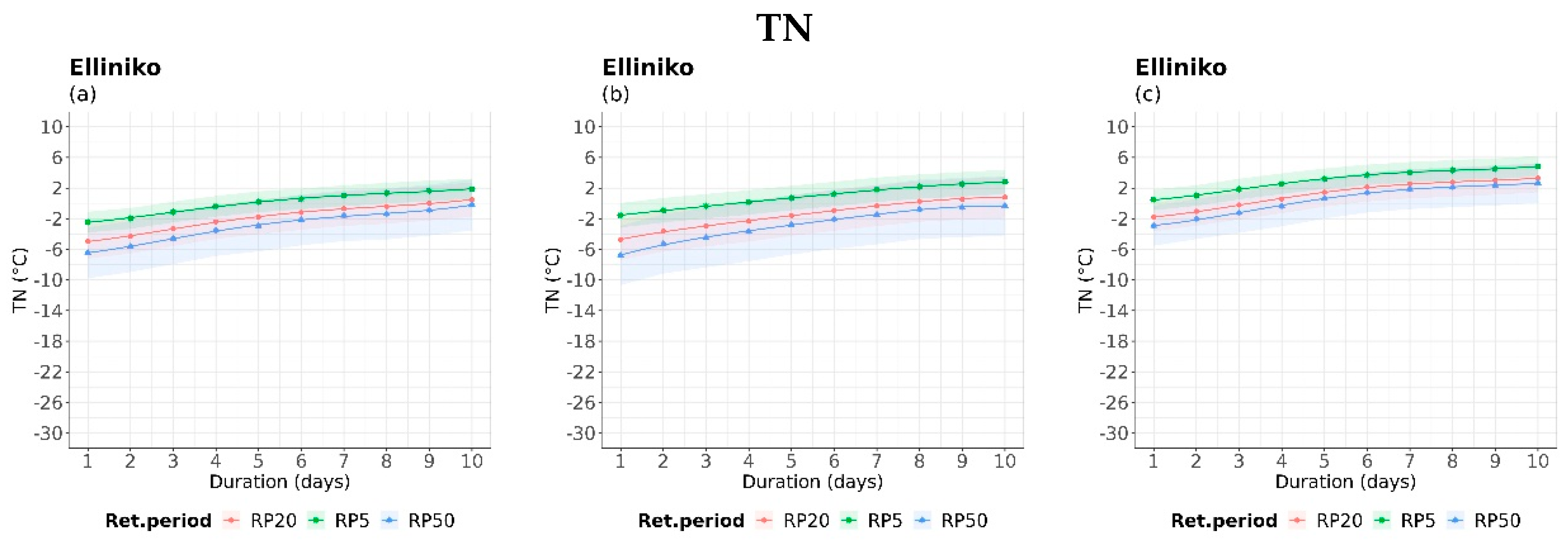
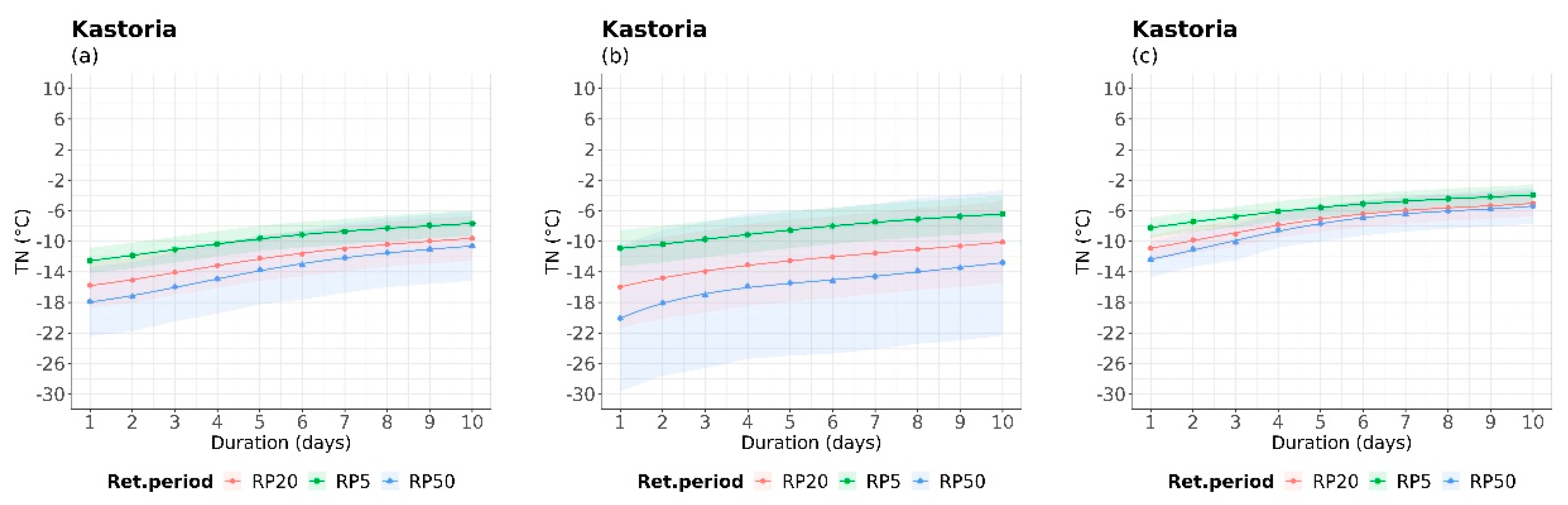
Figure 8.
IDRP curves of WSx for 5-, 20-, and 50-year return periods, during (a) the historical period (1980–2004), (b) near future period (2025–2049), and (c) far future (2075–2099) for indicative locations. The colored areas illustrate the 99% confidence intervals for each return period.
Figure 8.
IDRP curves of WSx for 5-, 20-, and 50-year return periods, during (a) the historical period (1980–2004), (b) near future period (2025–2049), and (c) far future (2075–2099) for indicative locations. The colored areas illustrate the 99% confidence intervals for each return period.
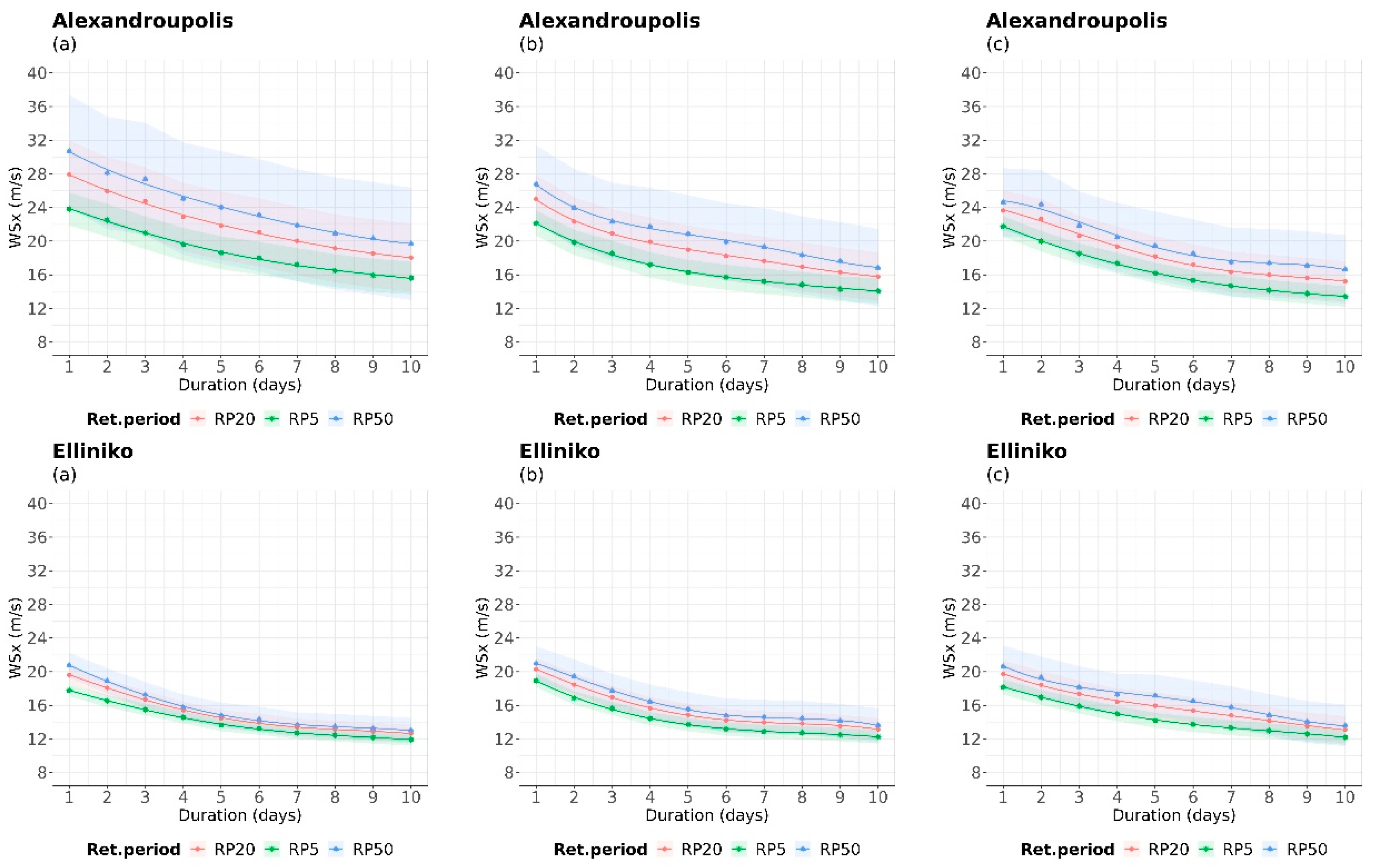
Figure 9.
IDRP curves of PR for 5-, 20-, and 50-year return periods, during (a) the historical period (1980–2004), (b) near future period (2025–2049), and (c) far future (2075–2099) for indicative locations. The colored areas illustrate the 99% confidence intervals for each return period.
Figure 9.
IDRP curves of PR for 5-, 20-, and 50-year return periods, during (a) the historical period (1980–2004), (b) near future period (2025–2049), and (c) far future (2075–2099) for indicative locations. The colored areas illustrate the 99% confidence intervals for each return period.

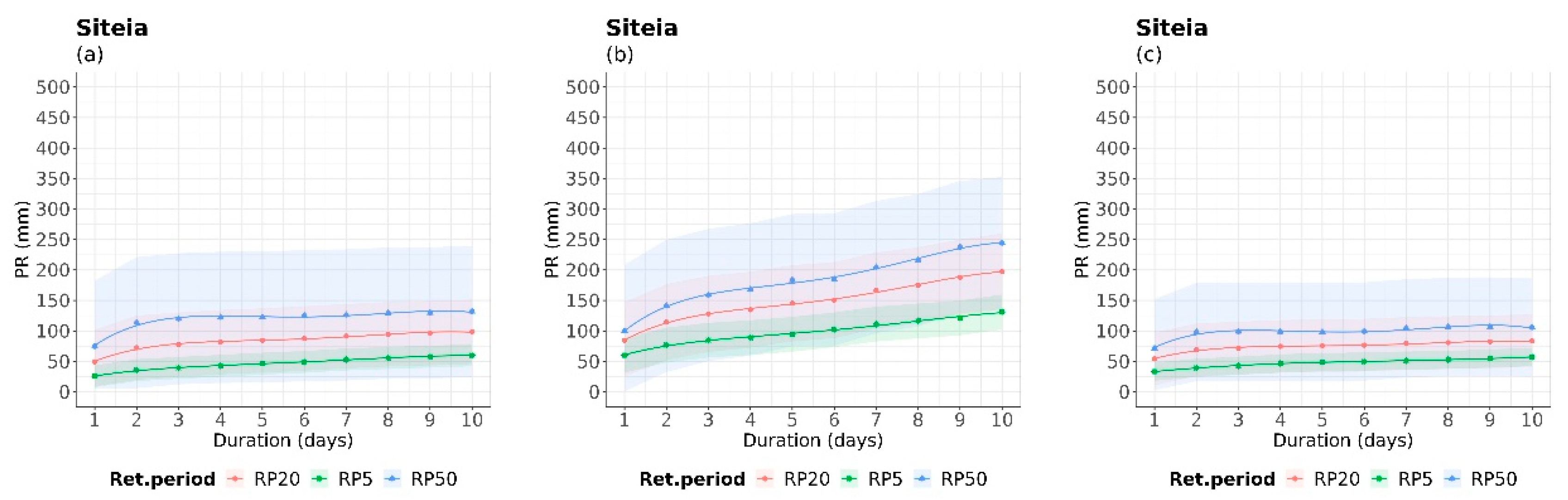
Figure 10.
IDRP curves of FWI for 5-, 20-, and 50-year return periods, during (a) the historical period (1980–2004), (b) near future period (2025–2049), and (c) far future (2075–2099) for indicative locations. The colored areas illustrate the 99% confidence intervals for each return period.
Figure 10.
IDRP curves of FWI for 5-, 20-, and 50-year return periods, during (a) the historical period (1980–2004), (b) near future period (2025–2049), and (c) far future (2075–2099) for indicative locations. The colored areas illustrate the 99% confidence intervals for each return period.

Table 1.
Collection of climate simulation daily data for the purpose of the study.
| Variables (Description) | Extreme Parameters | Duration Calculation |
|---|---|---|
| Maximum temperature | TX | Average |
| Minimum temperature | TN | Average |
| Precipitation | PR | Sum |
| Maximum snow | SNx | Sum |
| Maximum wind speed | WSx | Average |
| Fire weather index | FWI | Average |
Table 2.
Location of the HNMS station and model grid coordinates for this study.
| Stations/Location | Longitude | Latitude | Height (m) | WE | SN | HGT (Model) |
|---|---|---|---|---|---|---|
| Alexandroupolis | 25.917 | 40.85 | 4 | 118 | 149 | 10.1201 |
| Corfu | 19.912 | 39.603 | 1 | 21 | 114 | 6.96835 |
| Elliniko Airport | 23.7333 | 37.8877 | 10 | 89 | 81 | 117.431 |
| Larisa | 22.417 | 39.65 | 73 | 63 | 117 | 79.4701 |
| Naxos | 25.383 | 37.1 | 9 | 119 | 67 | 107.592 |
| Methoni | 21.7 | 36.8333 | 34 | 56 | 56 | 35.8098 |
| Siteia | 26.095 | 35.205 | 30 | 136 | 28 | 109.665 |
| Kastoria Airport | 21.28 | 40.45 | 660.95 | 43 | 133 | 656.411 |
Table 3.
Description of physical parameterization for the WRF model.
| Physics Parameterizations | |
|---|---|
| Microphysics scheme | WSM6, Hong and Lim 2006 [60] |
| Long-wave radiation scheme | RRTMG, Iacono et al. 2008 [61] |
| Short-wave radiation scheme | RRTMG, Iacono et al. 2008 |
| Planetary boundary layer scheme | MYJ, Janjic 2001 [62] |
| Surface layer | MO, Mellor and Yamada 1982 [63] |
| Cumulus scheme | BMJ, Betts and Miller 1986 [64] |
| Land surface model | NOAH, Chen and Dudhia 2001 [65] |
Table 4.
Intensity values for TX, TN, PR, WSX, SNX, and FWI for Kastoria, as estimated for the 20-year return period.
Table 4.
Intensity values for TX, TN, PR, WSX, SNX, and FWI for Kastoria, as estimated for the 20-year return period.
| RP20 | Duration (Days) | |||||||||
|---|---|---|---|---|---|---|---|---|---|---|
| 1 | 2 | 3 | 4 | 5 | 6 | 7 | 8 | 9 | 10 | |
| TX (°C) | 37.23 | 36.79 | 36.28 | 35.79 | 35.23 | 34.78 | 34.52 | 34.39 | 34.17 | 33.91 |
| TN (°C) | 15.75 | 15.09 | 14.07 | 13.17 | 12.21 | 11.65 | 10.99 | 10.38 | 9.96 | 9.62 |
| PR (mm) | 31.80 | 42.16 | 48.59 | 53.28 | 57.32 | 59.90 | 65.05 | 69.32 | 71.52 | 74.32 |
| WSX (m/s) | 22.04 | 19.14 | 16.86 | 15.17 | 13.93 | 12.84 | 12.32 | 11.97 | 11.52 | 11.13 |
| SNX (mm) | 12.42 | 17.37 | 21.09 | 25.07 | 30.04 | 30.98 | 32.60 | 32.79 | 34.53 | 37.71 |
| FWI | 78.23 | 63.44 | 57.28 | 53.70 | 51.70 | 50.13 | 48.36 | 46.66 | 45.71 | 44.82 |
Disclaimer/Publisher’s Note: The statements, opinions and data contained in all publications are solely those of the individual author(s) and contributor(s) and not of MDPI and/or the editor(s). MDPI and/or the editor(s) disclaim responsibility for any injury to people or property resulting from any ideas, methods, instructions or products referred to in the content. |
© 2023 by the authors. Licensee MDPI, Basel, Switzerland. This article is an open access article distributed under the terms and conditions of the Creative Commons Attribution (CC BY) license (https://creativecommons.org/licenses/by/4.0/).
Share and Cite
MDPI and ACS Style
Sfetsos, A.; Politi, N.; Vlachogiannis, D. Multi-Hazard Extreme Scenario Quantification Using Intensity, Duration, and Return Period Characteristics. Climate 2023, 11, 242. https://doi.org/10.3390/cli11120242
AMA Style
Sfetsos A, Politi N, Vlachogiannis D. Multi-Hazard Extreme Scenario Quantification Using Intensity, Duration, and Return Period Characteristics. Climate. 2023; 11(12):242. https://doi.org/10.3390/cli11120242
Chicago/Turabian StyleSfetsos, Athanasios, Nadia Politi, and Diamando Vlachogiannis. 2023. "Multi-Hazard Extreme Scenario Quantification Using Intensity, Duration, and Return Period Characteristics" Climate 11, no. 12: 242. https://doi.org/10.3390/cli11120242
Note that from the first issue of 2016, this journal uses article numbers instead of page numbers. See further details here.