Change in Heavy Rainfall Characteristics over the Ouémé River Basin, Benin Republic, West Africa

Abstract

Climate change has severe impacts on natural resources, food production and consequently on food security especially in developing countries. Likely accentuated by climate change, flooding is one of the disasters that affects people and destroies agricultural land and products. At different governance levels and scales, appropriate responses are needed. Cluster analysis using scaled at-site characteristics was used to determine homogeneous rainfall regions. A methodology for detecting change was applied to heavy daily rainfall of 34 stations across the Ouémé basin, Benin, in order to assess potential change in its characteristics. The spatial variability of the detected changes in return periods was analyzed using the kriging interpolation method. For this analysis, up to 92 years (1921–2012) of rainfall data were used. Three homogeneous regions were found by the cluster analysis. For all studied return periods, 82% of the stations showed statistically significant change in daily precipitation, among which 57% exhibited a positive change and 43% negative change. A positive change is associated with an increase in heavy rainfall over the area of concern. An analysis of the interpolated change in heavy rainfall of different return periods revealed an east-west gradient from negative to positive along the lower Ouémé basin (Region 2). From the middle to the upper Ouémé (Region 1 and 3), a decreasing tendency of heavy rainfall is dominant mainly for the non-homogeneous period. This result of the complex pattern of changes could be veritable information for decision makers and consequently for development of appropriate adaptation measures.

1. Introduction

Heavy rainfall events are one of the natural hazards that lead to degradation processes like flash floods or flooding as well as severe soil erosion, which can have regional devastating power and pose a serious hazard to lives and property. From 1900 to 2006, floods in Africa killed nearly 20,000 people and affected approximately 40 million more, and caused damage estimated at about US$4 billion [1]. In Benin, a number of extreme floods has occurred over the last 30 years and caused great economic losses. Between 1980 and 2009, there have been 14 major floods affecting a total of 2.26 million people [2]. According to the World Health Organization, an estimated 500 thousand people are at risk of flooding [3]. The floods in 2008 and 2009 caused widespread damage and displacement, affecting around 158 thousand and 120 thousand people, respectively [2]. Floods have become increasingly frequent, leading to the question of whether this was due to the increasing frequency of heavy rainfall or changes in land use patterns [4].

It is widely accepted that with the increase of temperature, the water cycling process will speed up, which in consequence will possibly result in the increase of precipitation amount and intensity [5]. Worldwide, efforts have been made to study the change direction of extreme rainfall as, for instance, in South America [6,7], in North America [8,9,10], in Europe [11,12,13,14,15,16], in Asia [5,17,18,19,20] and in Australia [21], among other regions in the world. The results of the previously cited works indicate that different directions of change in the frequency of heavy rainfall are possible.

Some areas of the globe have experienced an upward trend in extreme rainfall. For instance, Karl and Knight examined using a variety of methods how precipitation has changed over the United States and found that since 1910, precipitation has increased by about 10% [9]. They explained this fact by an increase in the frequency of days with precipitation and by an increase in intensity of the extremely heavy precipitation events. These results were confirmed by a study done by Kunkel and Andsager, which was extended to Canada where an upward trend was observed in extreme precipitation events [8]. All Europe-average indices of wet extremes increase in the 1946–1999 period, although the spatial coherence of the trends is low [13]. The same upward trend was observed in South America [6]. Significant increases in the intensity of extreme rainfall events between 1931–1960 and 1961–1990 are identified over about 70% of South Africa and the intensity of the 10-year high rainfall events has increased by more than 10% over large areas of this country, except in parts of the northeast, northwest and in the winter rainfall region of the southwest [22]. A combined work for Southern and West Africa performed by New et al. shows and confirms that regionally averaged rainfall on extreme precipitation days and maximum annual five-day and one-day rainfall amounts increase, but only the trend for the latter is statistically significant [23].

While evidence of increasing trends is presented for many regions, statistically significant decreasing trends in extreme rainfall events have also been found in other areas like the south of Europe [11], Southeast Asia and parts of the central Pacific [24], and in northern Nigeria [25].

In other parts, like China [26], no statistically significant change in heavy rain intensity is found. This is confirmed by the work of Wang et al. where little change is observed in various annual extreme precipitation indices, but significant changes are observed in the precipitation processes on a monthly basis, although the seasonal variations are not uniform even in a medium-sized basin such as the Dongxiang River Basin [5].

Until now, little is known about extreme rainfall over Benin. Yabi and Afouda examined recent years’ rainfall extremes and their socioeconomic and environmental impacts in Benin [27]. Their analysis showed strong incidence of extreme rainfall during the 1950s and 1960s, particularly in the south, while the 1970s and 1980s recorded very dry years. Hountondji and Ozer studied trends in extreme rainfall events in Benin for the period 1960–2000 using 12 rainfall indices [28]. They found that only the annual total precipitation, the annual total of wet days and the annual maximum rainfall recorded during 30 days present a significant decreasing trend while the other nine rainfall indicators appear to remain stable. Even though some efforts have been made to study extreme rainfall across the country, no study, as far as we know, investigated change in extreme rainfall over the country especially in the Ouémé basin by emphasizing on its frequency and its magnitude. The main objective of this work is to improve understanding of the heavy rainfall characteristics as key factor to support flood risk management in the Ouémé basin. This objective was split into three specific objectives: (a) identification of homogeneous regions in the study area through cluster analysis; (b) assessment of the frequency and/or intensity of extreme rainfall causing floods over the identified regions; and (c) interpolation of the point scale results to analyze the spatial pattern of change in heavy rainfall over the entire Ouémé basin. The Ouémé basin covers an area of about 50 thousand km² and 90% of this basin is located in Benin, West Africa.

2. Materials and Methods

The section presents the methodology used to analyze the heavy rainfall frequency and magnitude. It includes the data sampling approach, the determination of homogeneous regions though K-means clustering and the Principal Component Analysis (PCA), the extreme value distribution used namely the generalized Pareto distribution for quantile estimation, the kriging method for interpolation of the changes in return periods of heavy rainfall and some statistical tests.

2.1. Data Sampling

The rainfall data used in this study were obtained from the Benin national weather service (Direction Nationale de la Météorologie (DMN)) and cover the period of 1921 to 2012. Two approaches were investigated. As a first approach, only the stations having continuous record from 1951 to 2010 were selected for analysis. This period is referred to as “homogeneous period”. The term “homogeneous period“ implies that all the stations have the same data length (60 years) and are within the same range 1951–2010. Only the data of 17 stations were within this range (see Figure 1). This number of stations was not enough to perform statistical analysis and the regionalization (see Section 3.1.) over the area of about 50 thousand km² because using few stations could lead to high variance in the estimation. The minimum sample size required to have accurate results from statistical test is 30 [29]. Nevertheless, an analysis of the impact of the homogeneity in the study period on the results has been performed in Section 3.3.

The second approach was to consider the available data length for each station. In doing so, 34 stations with data length varying from 44 to 92 years have been chosen. This is referred to as “non-homogeneous period“ due to the difference in data lengths. The data records are within 1921–2012 (Figure 1).

For the non-homogeneous period, the data of each station are split into two sub-samples of equal length. Let X_j be the extreme values for one station such that X_j can be divided into two sub periods A_j and B_j with j varying from 1 to 34 (the number of stations). If we take X_j = x_i, x_i+1, …, x_N, where i ≥ 1921 and N ≤ 2012, we can define:

A_j = x_i, x_i+1, …, x_m

(1)

B_j = x_m+1, x_m+2, …, x_N

(2)

with m = (N + 1)/2 and this is rounded down to the nearest integer. This method was used for instance by Frich et al. [30]. x_i are extreme values corresponding to the year i.

2.2. Homogeneous Clusters

K-means clustering method combined with the principal component analysis (PCA) was used to determine homogeneous regions and their corresponding stations. This approach was chosen due to its successful application in other rainfall regionalization studies [31].

Different variables influence rainfall characteristics such as large-scale atmospheric variables of air temperature, geopotential height, specific humidity, zonal and meridional wind velocities, precipitable water and surface pressure in addition to latitude/longitude location, elevation and mean annual rainfall (MAR), at-site Mean Annual Precipitation (MAP), station latitude/longitude location, and elevation are proposed in the literature [31,32]. Due to the limited availability of some data, four characteristics available for the study area were used, namely the geographical location (latitude, longitude and altitude) and the MAP. Each variable was rescaled using the mean and the standard deviation of the corresponding variable in order to avoid bias of variables with large absolute values:

$$X_{i,j}=\frac{\left(Y_{i,j}-\overline{Y_j}\right)}{{\sigma }_j} for 1\le j\le n and 1\le i\le N$$

(3)

with $X_{i,j}$ and $Y_{i,j}$ the scaled and non-scaled values of the i-th station and the j-th variable, respectively, n is the total number of variables and N the number of stations or elements. The K-means algorithm minimizes the function $F$ defined below through an iterative procedure by moving the element from one cluster to another [31]:

$$F={\displaystyle \sum }_{k=1}^K{\displaystyle \sum }_{j=1}^n{\displaystyle \sum }_{i=1}^{N_k}{d}^2\left(X_{i,j}^k-X_j^k\right)$$

(4)

where the number of clusters K is set a priori; $N_k$ is the number of feature vectors (stations) in cluster k; $X_{i,j}^k$ denotes the rescaled value of attribute (variable) in the feature vector $i$ assigned to cluster k; and $X_j^k$ is the mean value of attribute j for cluster k, computed as:

$$X_j^k=\frac{{{\displaystyle \sum }}_{i=1}^{N_k}{X}_{i,j}^k}{N_k}$$

(5)

The number of clusters was determined using the Principal Component Analysis (PCA). The procedure first requires computation of the principal components of the sites’ precipitation records; i.e., the transformation of the sites’ precipitation records into a set of linearly uncorrelated (orthogonal) vectors [33]. The loadings indicate the degree of variance of the sites’ precipitation records that are described by each component; higher loadings are representative of greater variances. The loadings are contoured and the contoured areas that exceed a predefined threshold value are classified as coherent precipitation regions.

2.3. The Generalized Pareto Distribution

Two sampling methods are normally used in extreme events analysis: the annual maximal series (AMS) and the peak over threshold (POT) methods. The AMS considers only the greatest events in each year so the length of the AMS is equal to the number of record years. In contrast, the POT method considers all data in the series that are above a given threshold. Nevertheless, the issue of threshold choice implies a balance between bias and variance. A low threshold is likely to violate the asymptotic basis of the model, leading to a bias; a high threshold will generate few excesses with which the model can be estimated, leading to a high variance [34]. The standard practice is to adopt the threshold as low as possible that the model provides a reasonable approximation. Two methods are available for this purpose [34]: one is an exploratory technique carried out prior to model estimation; the other is an assessment of the stability of parameter estimates, based on the fitting of models across a range of different thresholds. In this study, the Peak over Threshold (POT) was adopted as sampling method. This choice was imposed by the data, which length were not sufficient to perform an analysis using the annual maximal approach for some of the stations.

The probability distribution of a POT variable with random occurrence times belonging to the Generalized Pareto family [35] with cumulative distribution F and quantile functions are:

$$\{\begin{array}{c}F\left(X\le x| \sigma ,k\right)=1-{\left[1+ k\left(\frac{x}{\sigma }\right)\right]}^{\frac{-1}{k}}; k\ne 0 and 1+ k\left(\frac{x}{\sigma }\right)>0 \\ F\left(X\le x| \sigma ,k\right)=1-exp\left(-\frac{x}{\sigma }\right) k=0, \sigma >0\end{array}$$

(6)

$$\{\begin{array}{c}{x}_{1-p}= F^{-1}\left(1-p;\sigma , k\right)=\left(\frac{\sigma }{ k}\right)(p^{- k}-1), 0<p<1, k\ne 0\\ x_{1-p}=F^{-1}\left(1-p;\sigma , k\right)=\sigma \log \left(\frac{1}{p}\right) k=0 \end{array}$$

(7)

where $p$ is the exceedance probability and ($1-p$) is the non-exceedance probability derived from the cumulative distribution function. $\sigma , k$ are, respectively, scale and shape parameters distribution, and x are the excesses over a selected threshold u [36]. The real quantile $y_{1-p}$ will be $y_{1-p}=x_{1-p}+u.$ If k > 0, then the Generalized Pareto Distribution (GPD) is heavy tailed. By convention, k = 0 refers to the limiting case obtained as $k\to 0$of the exponential distribution (i.e., an unbounded, thin tail).

Different thresholds were selected based on the minimum of the annual maximal sample of each station and the GPD fitted at each time by looking for stability in the estimated parameter values as suggested by Coles [34]. This condition is nearly satisfied for a daily rainfall amount of about 50 mm for the different datasets (see Appendix Figure A1, Figure A2, Figure A3, Figure A4, Figure A5, Figure A6, Figure A7, Figure A8, Figure A9 and Figure A10). Therefore the threshold of 50 mm is adopted for the following analysis.

The GPD was accordingly fitted to the data of each sub period$A_j$ and $B_j$. The Maximum Likelihood method was used for parameter estimation. For each station, the intensities ($I_{i=1:9}$) of 2-, 3-, 5-, 7-, 10-, 15-, 20-, 25-, and 30-year return periods were then obtained from the fitted distribution for each $A_j$ and $B_j$ periods and the percentage change $D_i^{\left(j\right)}$ (j−th station and i−th return period) in the intensities of the two periods was calculated using the following formula:

$$D_i^{\left(j\right)}=\frac{\left(I_i{\left(B_j\right)}_{ }-I_i\left(A_j\right)\right)}{I_i\left(B_j\right)} \times 100$$

(8)

where $I_i\left(A_j\right)$ is the i−th intensity computed for the first sub-period of the j−th station and $I_i\left(B_j\right)$ is the i−th intensity computed for the second sub-period of the j−th station.

The significance of changes in rainfall extremes was then assessed by comparing the mean of the difference in the intensity of heavy rainfall events with the difference expected under the null hypothesis. The null hypothesis states that there is no difference in the intensity of high rainfall events between $A_{n }$and $B_n$ periods. Two statistical tests were used for testing this significance: the Paired samples t-test [37] and the Wilcoxon test (paired samples) [38]. For detail about the computation of these tests, the reader can refer to references [37,38].

2.4. Hubert Segmentation Test, Kriging, Standardized Precipitation and Extreme Precipitation Indexes

To determine change points in the number of heavy rainfall days above some thresholds per year, we applied the Hubert Segmentation Test. Its principle is to split the data into m segments (m > 1) in such a way that the mean computed over a segment is different from the mean of the neighboring segment.

Let $X_i \{i=i_1,i_2 ;1<i_1 and i_2<N with i_1<i_2\}$ be a segment of the initial series of data. From a particular segmentation of order m done on the initial data, we can define [39]$i_{k\left\{k = 1, 2, \dots ,m\right\}}$, as the rank of the initial series extremity of the kth segment; $\overline{x_k} ,$as the mean of the k-th segment; and $D_m,$ as the square of the difference between the data and the segmentation considered, where

$$D_m={\displaystyle \sum }_{k=1}^m{d}_k with d_k={\displaystyle \sum }_{i=i_{k-1}+1}^{i_k}{\left(x_i-\overline{x_i}\right)}^2$$

(9)

The algorithm tries to minimize $D_m$ and the means of continuous segments must be significantly different. This later constrain is satisfied by applying the test of Scheffé [39].

The interpolation of change in heavy rainfall magnitude was done using the kriging method. Kriging is a linear interpolation method that allows estimating areal values as a weighted mean of the point observations [40]. The weights attributed to the different observations depend on the variability structure of the variable. This variability structure is taken into account using the variogram function, which is the difference between the variance and the covariance function. Empirical variograms are calculated using the observation datasets and then a variogram model is fitted. For each grid cell, using the variogram model, a linear system yields the interpolation weights attributed to the observation points. For a detailed presentation of theoretical and practical issues related to kriging, see, for example, reference [41].

The standardized precipitation index (SPI) and the standardized extreme precipitation index (SEPI) was used to analysis the correlation between the annual rainfall and the extreme rainfall. The SPI is defined as:

$$X_{i,j}=\frac{Y_{i,j}-\overline{Y_i}}{{\sigma }_i}$$

(10)

where $X_{i,j}$ is the SPI of the year $j$ at the station$i$, $Y_{i,j}$ is the annual rainfall of the year $j$ at the station $i$, $\overline{Y_i}$is the mean annual rainfall at the station $i$ and ${\sigma }_i$ is the standard deviation of the mean annual rainfall at the station $i$. The SEPI is computed in a similar manner by considering the series of maximum annual rainfall at each station.

3. Results and Discussion

3.1. Identification of Homogeneous Regions

In the application of K-means clustering, the number of clusters or groups must be set a priori. The PCA was used to find the number of components based on the longitude, the latitude, the altitude and the mean annual rainfall (MAR) of each station.

Table 1. Importance of principal components (PC).

Components and Statistics	PC1	PC2	PC3	PC4
Standard Deviation	1.4	1.0	0.9	0.3
Proportion of Variance	0.5	0.28	0.21	0.02
Cumulative Proportion	0.49	0.76	0.98	1

shows the importance of each principal component (PC). The three first components explained more than 97% of the variance of the data. This suggests that using three groups was sufficient to reproduce most of the variance in the dataset. Based on this, the number of clusters was set to three during the K-means clustering. Figure 2 shows the stations of each group (cluster).

Group 1 had nine stations located in the northeast of the basin with a mean annual rainfall of 1084 mm and an average altitude of 360 m above sea level. Most of the stations of this group are located in a unimodal rainfall regime. Group 2 was comprised of fifteen stations located in the south of the basin with mean annual rainfall of 1079 mm and an average altitude of 169 m. This group was located in a bimodal rainfall regime. Group 3 had ten stations located in the western part of the basin with mean annual rainfall of 1187 mm and a mean altitude above sea level of 378 m. The mean annual rainfall was computed for the period 1970 to 2010 ignoring the years having more than 10% of data missing.

3.2. Significance of Change in Heavy Rainfall over Ouémé Basin

The Paired samples t-test and Wilcoxon test (paired samples) were both applied to the difference in the rainfall intensities of each station. A change is considered if it has been detected by both tests. Considering the results obtained from the non-homogeneous period and for all studied return periods, 82% of the stations show statistically significant change at 99% confidence level (corresponding to alpha = 1% significance level). This means that heavy rainfall over the study area has statistically changed at 82% of the stations. Among the statistically significant changes, 57% of the stations exhibit a positive change and 43% a negative change. Considering the mean percentage change for all return periods, the highest positive change was observed at the station of Tchètti while the highest negative change was observed at Savè.

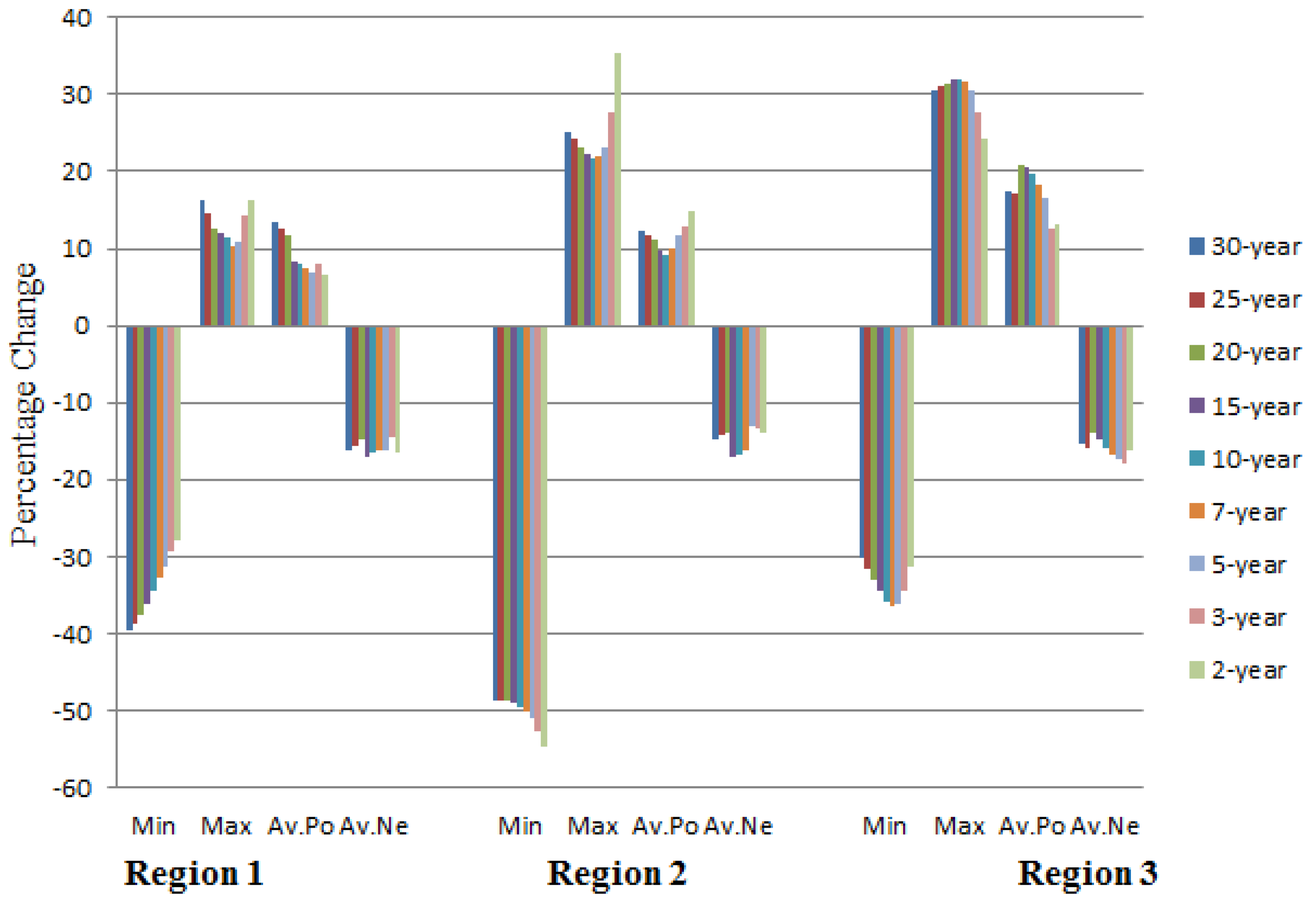
Analysis of the spatial variation of change was done based on the three rainfall regions found during the cluster analysis. Figure 3 shows the maximum, the minimum and the averages of positive and negative changes by region for each return quantile. There is no clear pattern about the change direction of heavy rainfall in the different regions since positive as well as negative changes were found. Nevertheless, for all regions, the maximum negative percentage changes were greater in magnitude than the maximum positive changes for most of the return periods. The highest negative changes were found in Region 2 while the highest positive changes were observed in Region 3 similarly to what was obtained for the mean annual rainfall of these regions.

In Region 1, for all the studied return periods, the average negative change varied between −15% and −17% while the maximum positive change varied between 7% (two-year) and 13% (30-year). The average negative changes were stable for the different return periods compared to the average positive changes which increased with the return periods.

In Region 2, the average negative changes varied between –13% (five-year) and –17% (15-year) when the average positive changes varied between 9% (10-year) and 15% (two-year). For the positive percentage change, there was a decreasing trend from 30-year to 10-year before increasing up to two-year return period. No clear trend was found in the average negative changes in this region.

In Region 3, the average negative changes varied between −14% (20-year) to −18% (three-year) and the average positive changes varied between 13% (three-year) and 21% (20-year). A decreasing trend is observed from 20-year to two-year return period for the average positive percentage change.

Overall, positive as well as negative changes are balanced in the basin. This kind of mixed pattern of changes is also observed in other parts of world. Bates et al. [42] report that generally, the frequency of occurrence of more intense rainfall events in many parts of Asia has increased, causing severe floods, landslides, and debris and mud flows, while the number of rainy days and total annual amount of precipitation have decreased. However, they also report that the frequency of extreme rainfall in some countries of Asia has exhibited a decreasing tendency. Increased precipitation intensity and variability can increase the risks of flooding. The frequency of heavy precipitation events (or proportion of total rainfall from heavy falls) will be very likely to increase over most areas during the 21st century, with consequences for the risk of rain-generated floods.

3.3. Spatial Pattern of Change in Heavy Rainfall in the Study Area

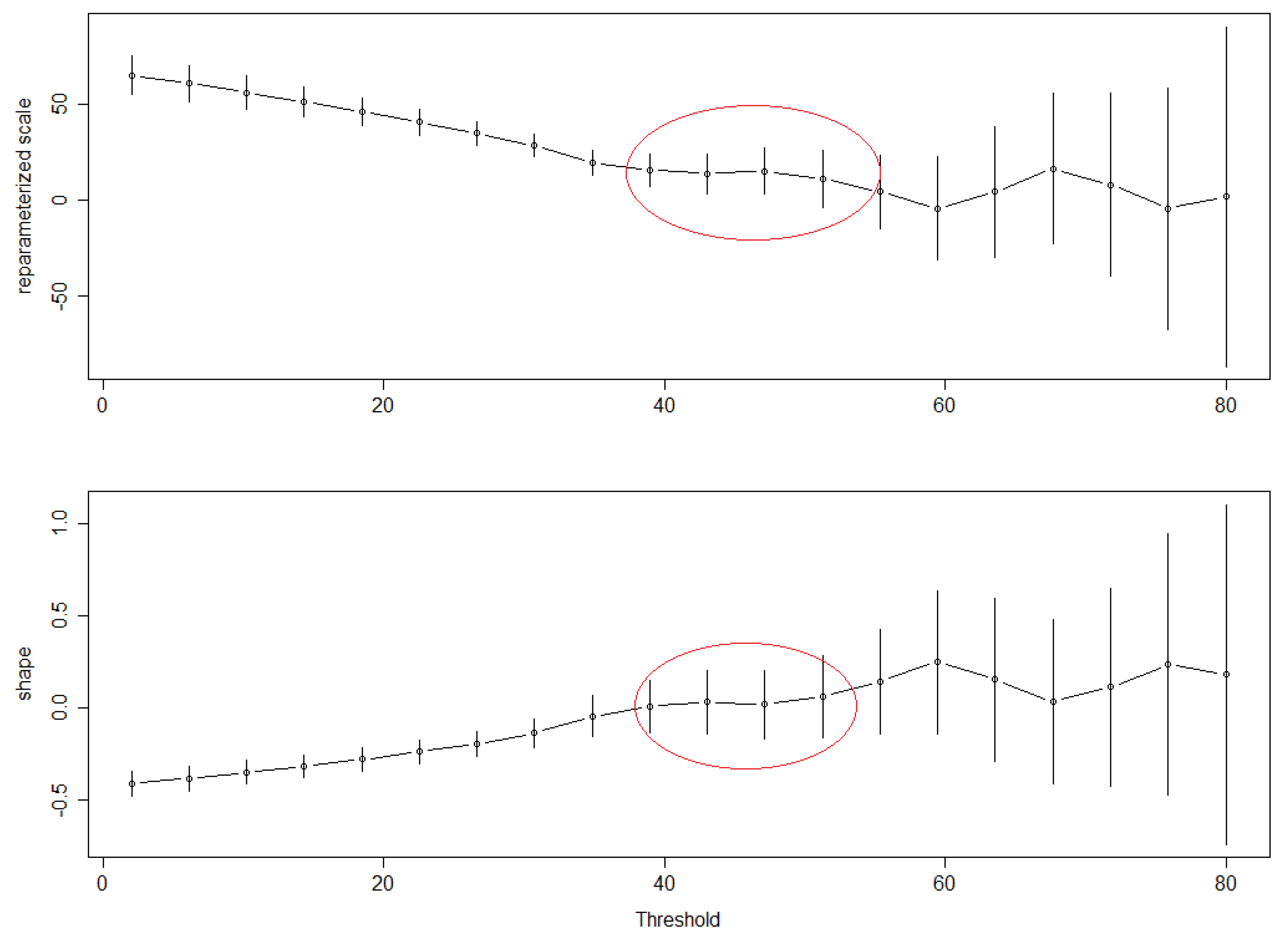
Spatial interpolation of change in heavy rainfall was done using the kriging method. Different models used to approximate the variogram corresponding to each return period were the spherical, circular and stable models (see Appendix Figure A11 for the model variograms). Figure 4 shows the map of change in different return periods of heavy rainfall over the Ouémé basin. Generally, the rainfall change-based map shows a mixed pattern of positive and negative changes for the different return periods plotted. Firstly, an east–west gradient from negative to positive was observed along Region 2. Along the western part of this region, high increases in the intensity of heavy rainfall events have been experienced despite the negative rainfall index meaning decreasing in annual rainfall since 1970 over West Africa [43]. This case study shows that, depending on the threshold used to define dry period, the increase in the frequency of dry spell (statistically significant) observed in large part of Sub-Saharan Africa, particularly in Benin [44], does not necessarily mean a decrease in the frequency of extreme heavy-rainfall events. In the eastern part of Region 2, decreases in heavy rainfall were observed for the different return periods and it is accentuated around the eastern part of the region. This change at the southeast of the basin is to be taken with precaution since we do not have enough stations in this region to represent the spatial variability.

For Regions 1 and 3, no general pattern was found. Nevertheless, the decreasing tendency was dominant sprinkled with some local increase in heavy rainfall for the different return periods. This is in accordance with the finding of Hountondji and Ozer (2000) about the annual maximum rainfall recorded during 30 days in Benin. Similarly, downward trend in the extreme rainfall was observed by Soro across part of Ivory Coast [45], and by Tarhule and Woo in Nigeria [25], which are located in almost the same climate region of the study area (Golf of Guinea). Groisman et al. [46] show that a general decreasing trend in heavy rainfall exists over West Africa. This downward trend, even if it is not over the entire basin is in accordance with the finding of Goula et al. for Ivory Coast [47] and Mason et al. for South Africa [22] where the direction of changes in extreme rainfall follows the one of total annual rainfall (see Section 3.6).

Overall, similar spatial patterns of change were found for the different return periods analyzed but the magnitude and the spatial extent of change differed from one return period to another mostly for Region 1 and Region 3. As reported by Bates et al., changes in extremes, including floods and droughts, are projected to affect water quality and exacerbate many forms of water pollution, including sediments, nutrients, dissolved organic carbon, pathogens, pesticides and salt, as well as thermal pollution, with possible negative impacts on ecosystems, human health, and water system reliability [42]. Thus, different adaptation measures should be implemented in order to reduce the negative impact this change could have in different sectors such as agriculture, health, transportation etc. Some areas in the different homogeneous regions showed very high change in term of magnitude of positive and negative percentage change. The frequency of rainfall in these areas is analyzed in the next section.

3.4. Frequency of Heavy Rainfall at Stations with Highest Changes

More investigation was done about the areas showing the highest positive and negative changes in heavy rainfall. We concentrated on the rainfall stations having the two highest negative changes and the two highest positive changes (Region 1: Nikki; Region 2: Savè and Ouèssè; and Region 3: Tchètti). We computed the number of days with rainfall greater or equal to 50 mm over the available data length and applied the Hubert segmentation test [48] to each sample. The choice of this index is justified by the fact that it helps to better understand the frequency of extreme rainfall [47]. Figure 5 shows the plot of the number of days where the daily rainfall is greater or equal to 50 mm at Savè and Nikki (highest negative change stations), and Ouèssè and Tchètti (highest positive change stations) with the Hubert segments. A break point was found in 1936 for the station of Savè. The number of heavy rainfall days during the period 1921–1936 was very high with an average of 13 heavy rainfall days per year compared with an average of three days during the period of 1937–2012. This implies that the first period received more extreme rainfall than the second period. At Tchètti, the Hubert segmentation test found a break in 2004 with an average of four heavy rainfall days per year during the period 1964–2004 while the period 2005–2012 experienced on average more than seven heavy rainfall days per year. This shows that less heavy rainfall fell during the first period in comparison with the second period. For Nikki and Ouèssè, similar changes are found in comparison, respectively, with Savè and Tchètti (see Figure 5).

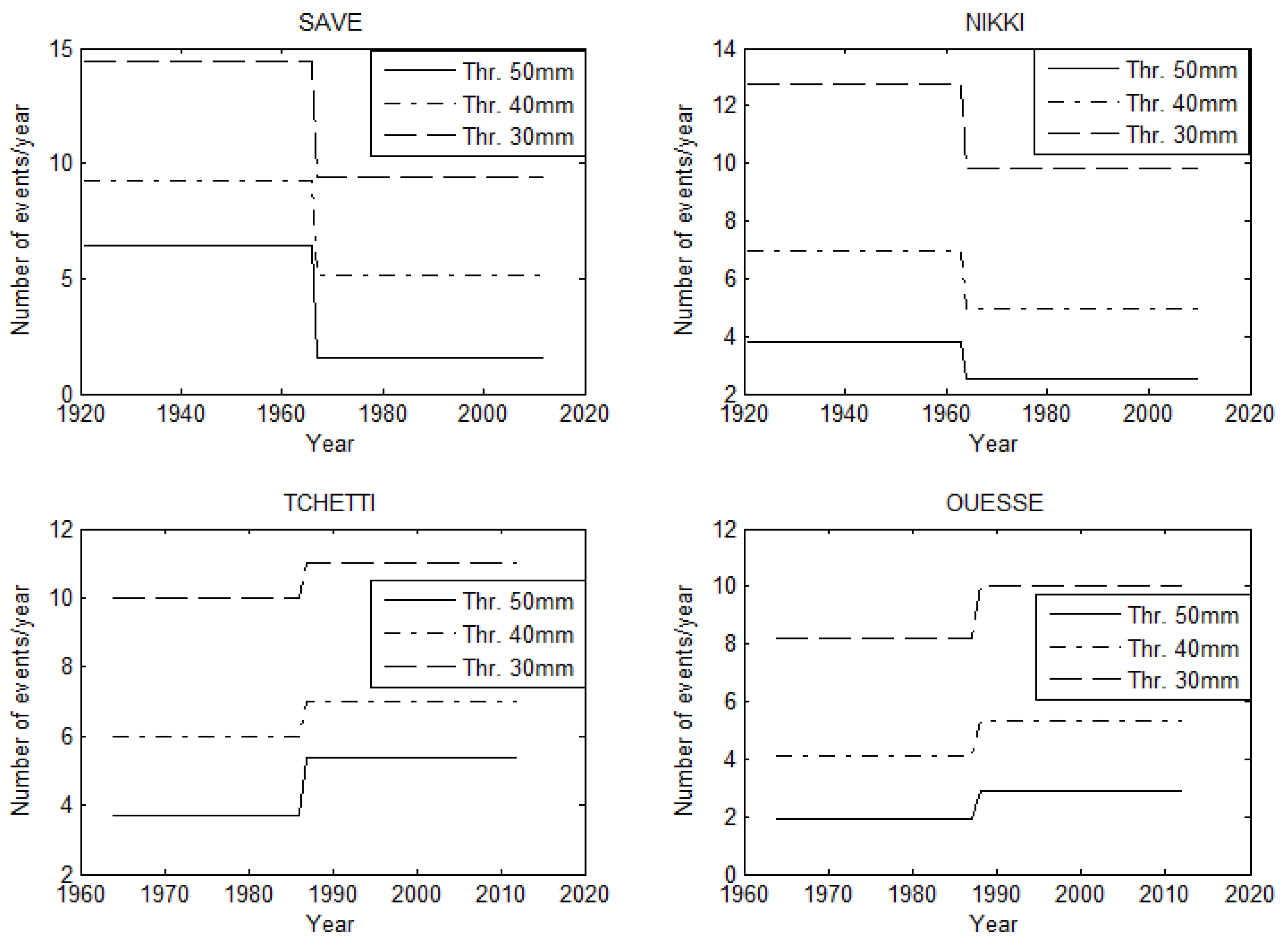
When we consider the sub-periods used under the “non-homogeneous period” for the station of Savè, the average of high rainfall days per year was 6.41 during the period 1921–1966 and 2.63 during the period 1967–2012. The first was more than the double of the second period. This shows that the first period was very wet compared with the second period and explains largely the high negative percentage change found for this station. Similarly, under the non-homogeneous period, Nikki exhibited an average of 3.8 high rainfall days per year during the first sub period and 2.5 heavy rainfall days per year during the second sub period (Figure 6). Indeed, heavy rainfalls have become less frequent than previously observed in that region. In the same way, the high decrease in the heavy rainfall could be explained by the reduction in the number of heavy rainfall days per year.

As far as the other two stations were concerned and considering the threshold of 50 mm, an average of 3.7 and 1.9 heavy rainfall days were found for Tchètti and Ouèssè, respectively, for the first period. For the second period, 5.4 and 2.9 are, respectively, the number of rainfall days for Tchètti and Ouèssè. Contrary to what has been found for the first two stations, the second period was wetter than the first period for these stations. There was an increase in the number of heavy rainfall days per year in these areas, which explains the positive change in heavy rainfall found.

In addition, two thresholds (40 and 30 mm) were added to investigate whether the change direction (sign of the change) would vary depending on the threshold. Low thresholds were chosen since such amounts (less than 50 mm) of rainfall may lead to flash floods, depending on the morphology of the region and precedent soil moisture condition. As can be seen in Figure 6, the change direction remained the same when we vary the threshold meaning that the results obtained were independent of the choice of the threshold.

3.5. Influence of Homogeneity of the Study Period on the Change

In the study of climate change impact, homogeneous periods (same data length and the same range) are required. In data scarce regions like West Africa, satisfying this condition is sometimes difficult, making the results of the study uncertain. Through this, a homogeneous period (1951–2010) has been used to compare the results with the non-homogeneous period (different data length) used before. The previous methodology was applied considering the same data length (1951–2010) for all stations. Seventy-three percent of the stations show a statistically significant change at 99% confidence level compared to the 82% in the non-homogeneous period. Considering the non-homogeneous period with length up to 92 years, which was much longer than the one of homogeneous period, the difference in the number of stations showing significant change means that, long term changes in heavy rainfall is stronger than recent changes. Figure 7 shows the percentage change of two-, five- and 10-year heavy rainfall for homogeneous period as well as for the non-homogeneous period. As can be seen, there was a high difference between the spatial patterns of the two sets of map. For the homogeneous period, most of the changes for the different return periods were negative, meaning that there was a decreasing tendency in heavy rainfall. Nevertheless, positive changes were partially observed in the northern and southwestern parts of the basin. Due to the limited number of stations used for the homogeneous period, the result of this interpolation should be taken with caution. For the non-homogeneous period, there was a mixed pattern of positive and negative changes. In the southwest of the basin, there was higher increase in heavy rainfall for the non-homogeneous (>17%) than the homogeneous (<10%) periods. In the same way, the maximum negative change for the non-homogeneous period is greater in magnitude than the maximum negative change for the homogeneous period. In comparison with the non-homogeneous period, which was longer (1921–2012), this homogeneous period helps to quantify recent change in extreme rainfall (1951–2010). Whatever the chosen period (homogeneous or non-homogeneous) and return periods were, it was found that the decreasing tendency was dominant in term of spatial distribution. The major difference was in the intensity of this change, which was less accentuated with the homogeneous period than the non-homogeneous one.

There is a contrast between the station-based results and the interpolation. Indeed, for the at-site based results, the number of stations showing statistically positive change was greater than the one showing negative change for the non-homogeneous period. In contrast, after the spatial interpolation, the area covered by positive change is less than the corresponding area for the negative change. This may be due the fact that the maximum of positive change is low, sometimes lower than one-third of the absolute maximum negative for all return periods. This gave more weight to the negative values during the interpolation than the positive values. The model variogram for the kriging was an approximation of the observed variogram and this approximation became more accurate with the number of observation sites. Due to the limited number of stations used, the uncertainties in the estimation may be high.

3.6. Extreme Rainfall and Annual Total Rainfall

We computed the correlation coefficient between the annual rainfall and the annual maximal rainfall considering for each station, the years having less than 10% of data missing. Over the 34 rainfall stations in the study area, we found 29 stations showing statistically significant correlation coefficient at 95% confidence level. These coefficients vary from 0.3 at Kétou station to 0.75 at Savè station (

Table 2. Correlation coefficient between the annual maximal rainfall and the annual rainfall, and the corresponding p-value, as well as the correlation coefficient between the annual rainfall and the number of rainy days with rainfall amount greater or equal to 50 mm.

Stations	Annual Maximal Rainfall and Annual Total Rainfall		Number of Rainy Days > 50 mm and Annual Total Rainfall
	Correlation	p-Value	Correlation	p-Value
Abomey	0.50	7.84E−07	0.52	1.57E−07
Agouna *	0.20	2.41E−01	0.76	9.56E−08
Aklankpa	0.68	9.54E−04	0.72	3.03E−04
Bantè *	0.19	1.21E−01	0.54	2.30E−06
Bassila	0.52	5.45E−04	0.68	8.77E−07
Bembèrèkè	0.50	5.81E−07	0.71	3.58E−15
Bétérou	0.45	1.18E−03	0.70	2.25E−08
Birni	0.39	9.43E−03	0.68	4.04E−07
Bohicon	0.46	5.36E−05	0.64	2.66E−09
Bonou	0.32	3.90E−02	0.72	1.20E−07
Dassa-Zoumé	0.44	3.07E−04	0.75	2.67E−12
Djougou	0.50	3.93E−06	0.80	9.31E−19
Gouka	0.38	1.59E−02	0.68	1.54E−06
Ina	0.38	5.41E−03	0.62	6.98E−07
Kalalé	0.68	1.68E−07	0.69	9.59E−08
Kétou	0.30	2.42E−02	0.74	1.42E−11
Kokoro	0.43	7.83E−03	0.81	1.56E−09
Kouandé	0.44	7.44E−05	0.68	1.42E−11
Lonkly	0.43	1.06E−03	0.71	1.10E−09
Niaouli	0.47	4.67E−05	0.76	7.91E−14
Nikki	0.46	2.90E−05	0.64	5.10E−10
Okpara *	0.19	1.73E−01	0.65	1.24E−07
Ouèssè	0.60	6.01E−06	0.62	2.44E−06
Parakou	0.35	7.53E−04	0.63	8.39E−11
Patargo	0.73	2.49E−04	0.81	1.69E−05
Pénéssoulou *	0.42	5.12E−02	0.38	8.17E−02
Pira	0.49	1.37E−03	0.72	1.32E−07
Savalou	0.51	3.87E−06	0.79	7.66E−17
Savè	0.75	1.76E−17	0.94	1.64E−41
Sèmèrè	0.51	7.96E−03	0.82	3.43E−07
Tchaourou	0.46	2.36E−04	0.76	5.80E−12
Tchètti *	0.24	1.89E−01	0.79	5.67E−08
Toui	0.41	1.40E−03	0.49	8.50E−05
Zagnanado	0.36	9.76E−04	0.77	1.52E−17

* No statistically significant correlation at 5% significance level.

). Eleven stations have a correlation coefficient greater 0.5. This implies that an annual maximum increases with the annual rainfall amount. A typical example was the station of Savè where the trend in extreme rainfall was similar to the one of annual rainfall.

Additionally, we found high and statistically significant (at 5% significance level) correlation between the number of heavy rainfall days per year and the total annual rainfall for all stations except Pénéssoulou (Table 2). Precipitation seems to be concentrated in more intense events, with more or less longer periods of lower precipitation in between. Therefore, intense and heavy episodic rainfall events with high runoff amounts were interspersed with longer relatively dry periods with increased evapotranspiration.

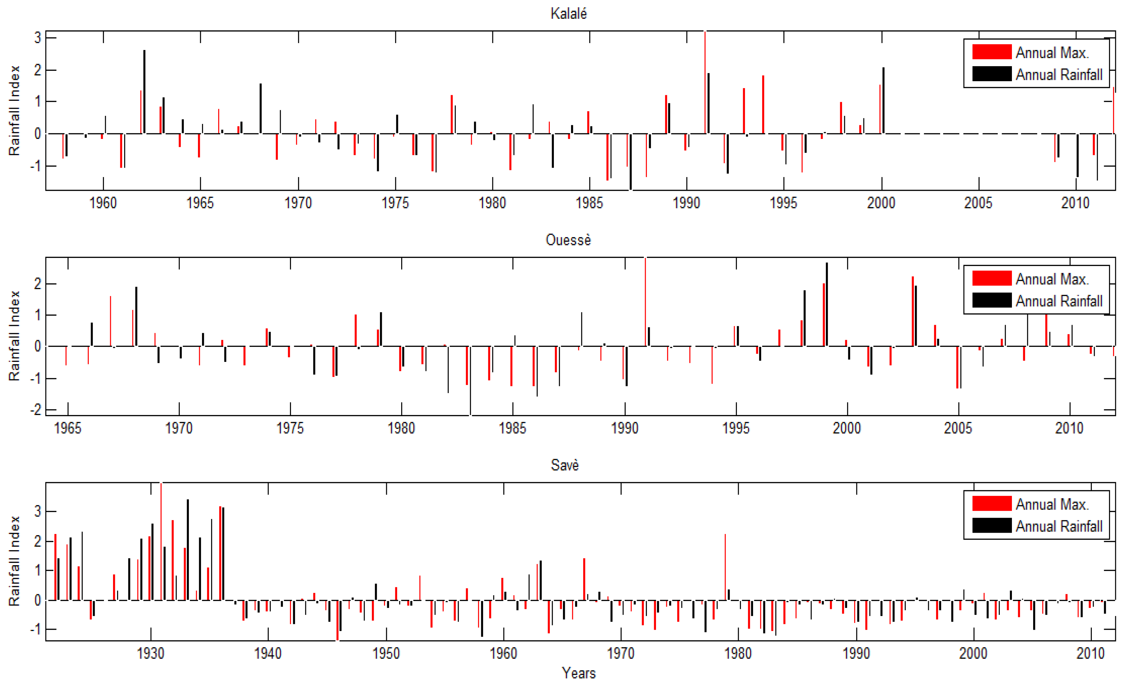
In order to better capture the dynamic between the two variables, we computed the standardized precipitation index (SPI) and the standardized extreme precipitation index (SEPI). Figure 8 show the SPI and the SEPI for three stations. It is interesting to note that for all stations, a positive SPI is mostly accompanied by a positive SEPI and a negative SPI is mostly accompanied by a negative SEPI. In other words, an increase in annual rainfall leads to an increase in extreme rainfall. When we consider the case of Savè (Figure 8), between 1922 and 1936, SPI and SEPI were all positive (except the year 1925) and most values exceeded the standard deviation of the corresponding variable with the highest index (for SPI) being almost four times the standard deviation of the annual rainfall. The high and positive indexes found reveal that this period was very wet and accompanied with very heavy rainfall. From 1936 to 2012, most of the SPI and SEPI had the same sign. An overall 75% of the SPI and SEPI between 1922 and 2012 exhibited a change of the same direction at Savè station. At Kalalé station, 66% of the SPI and SEPI showed the same direction changes, while for Ouèssè it was 63%.

4. Conclusions

In this paper, K-means and PCA clustering analyses were performed and three homogeneous rainfall regions were found in the Ouémé basin. We then explored changes in heavy rainfall following the peak over threshold approach using the generalized Pareto distribution. The data of each station were split into two sub-periods and the model was then fitted to the data of each sub-period. Change in extreme rainfall was then assessed by computing the difference in the intensities of the two sub-periods. As has been observed in other parts of the word, the frequency of extreme rainfall has changed over the study area. Significant negative as well as positive changes have been found throughout the basin. For the non-homogeneous period, 82% of the stations show a statistically significant change, among which 57% exhibit a positive change and 43% negative change. A positive change is associated with an increase in heavy rainfall over the area of concerned.

A spatial interpolation of heavy rainfall corresponding to different return periods was done and it was found that the southwestern part of the basin shows an increasing tendency in heavy rainfall while a decreasing tendency was observed in the middle and upper parts, sprinkled with some upward trend. It was also found that whatever the chosen period (homogeneous or non-homogeneous) and return periods were, the decreasing tendency is dominant in terms of spatial distribution. The major difference was in the intensity of this change, which was more accentuated with the non-homogeneous period than the homogeneous one. Another difference is in the intensity of the positive change, which was more pronounced with the non-homogeneous period than the homogeneous one. Additionally, we found high and statistically significant (at 5% significance level) correlation between the number of heavy rainfall days per year and the total annual rainfall for all stations except Pénéssoulou.

The impacts of changes in the frequency of floods could be tempered by appropriate infrastructure investments, and by changes in water and land-use management. Change in flood frequency and magnitude can have positive and negative impacts. It is important, therefore, to be aware of its consequences at local and national levels and to plan accordingly. The expected continuation of rapid population growth will increase human exposure to flooding and adequate adaptation measure must be implemented.

With the mixed pattern of change (increase and decreasing tendency) observed at different return periods for the heavy rainfall, we can deduce that climates factors may not be the main element contributing to increasing flood risk in this basin. This is in line with previous research on high discharge over the same basin, which revealed no significant increase in the annual maximum discharge at 5% significance level [49]. More investigations are needed to explain the recent flood inundation observed over the Ouémé basin and at the national level. This may be an analysis of whether this situation (flooding condition) is accentuated by changes in land use patterns and/or by the vulnerability of the population.

References

1. Davidson, O.; Chenene, M.; Kituyi, E.; Nkomo, J.; Turner, C.; Sebitosi, B. Sustainable Energy in Sub-Saharan Africa. Available online: http://www.icsu.org/icsu-africa/publications/ICSUROASciencePlanonSustainableEnergy.pdf (accessed on 11 October 2015).
2. EM-DAT: The International Disaster Database. Available online: www.emdat.be (accessed on 23 September 2013).
3. UNOCHA Benin: Half Million Potential Flood Victims: WHO. Available online: http://www.irinnews.org/report/80153/benin-half-million-potential-flood-victims-who (accessed on 3 September 2008).
4. Hounkpè, J.; Diekkrüger, B.; Badou, D.; Afouda, A. Non-stationary flood frequency analysis in the Ouémé River Basin, Benin Republic. Hydrology 2015, 2, 210–229. [Google Scholar] [CrossRef]
5. Wang, W.; Chen, X.; Shi, P.; van Gelder, P.H.A.J.M. Detecting changes in extreme precipitation and extreme streamflow in the Dongjiang River Basin in southern China. Hydrol. Earth Syst. Sci. 2008, 12, 207–221. [Google Scholar] [CrossRef]
6. Re, M.; Barros, V.R. Extreme rainfalls in SE South America. Clim. Change 2009, 96, 119–136. [Google Scholar] [CrossRef]
7. Carvalho, L.M.V.; Jones, C.; Liebmann, B. Extreme precipitation events in Southeastern South America and large-scale convective patterns in the South Atlantic Convergence Zone. J. Clim. 2002, 15, 2377–2394. [Google Scholar] [CrossRef]
8. Kunkel, K.E.; Andsager, K. Long-term trends in extreme precipitation events over the conterminous United States and Canada. J. Clim. 1999, 12, 2515–2527. [Google Scholar] [CrossRef]
9. Karl, T.R.; Knight, R.W. Secular trends of precipitation amount, frequency, and intensity in the United States. Bull. Amer. Meteor. Soc. 1998, 79, 231–241. [Google Scholar] [CrossRef]
10. Feng, S.; Hu, Q. Changes in winter snowfall/precipitation ratio in the contiguous United States. J. Geophys. Res. 2007, 112, 1–12. [Google Scholar] [CrossRef]
11. Frei, C.; Scho, R.; Fukutome, S.; Vidale, P.L. Future change of precipitation extremes in Europe: Intercomparison of scenarios from regional climate models. J. Geophys. Res. 2006, 111. [Google Scholar] [CrossRef]
12. Kyselý, J.; Beranová, R. Climate-change effects on extreme precipitation in central Europe: Uncertainties of scenarios based on regional climate models. Theor. Appl. Clim. 2009, 95, 361–374. [Google Scholar] [CrossRef]
13. Klein Tank, A.M.G.; Koennen, G.P. Trends in indices of daily temperature and precipitation extremes in Europe. J. Clim. 2003, 16, 3665–3680. [Google Scholar] [CrossRef]
14. Beguería, S.; Angulo-Martínez, M.; Vicente-Serrano, S.M.; López-Moreno, J.I.; El-kenawy, A. Assessing trends in extreme precipitation events intensity and magnitude using non-stationary peaks-over-threshold analysis: A case study in northeast Spain from 1930 to 2006. Int. J. Climatol. 2011, 31, 2102–2114. [Google Scholar] [CrossRef] [Green Version]
15. Ramos, M.C.; Martínez-Casasnovas, J. Trends in precipitation concentration and extremes in the Mediterranean Penedès-Anoia Region, Ne Spain. Clim. Change 2006, 74, 457–474. [Google Scholar] [CrossRef]
16. Burt, T.; Weerasinghe, K. Rainfall distributions in Sri Lanka in time and space: An analysis based on daily rainfall data. Climate 2014, 2, 242–263. [Google Scholar] [CrossRef] [Green Version]
17. May, W. Variability and extremes of daily rainfall during the Indian summer monsoon in the period 1901–1989. Glob. Planet. Change 2004, 44, 83–105. [Google Scholar] [CrossRef]
18. Zhang, Q.; Sun, P.; Chen, X.; Jiang, T. Hydrological extremes in the Poyang Lake basin, China: Changing properties, causes and impacts. Hydrol. Process 2011, 25, 3121–3130. [Google Scholar] [CrossRef]
19. Panthi, J.; Dahal, P.; Shrestha, M.; Aryal, S.; Krakauer, N.; Pradhanang, S.; Lakhankar, T.; Jha, A.; Sharma, M.; Karki, R. Spatial and temporal variability of rainfall in the Gandaki River Basin of Nepal Himalaya. Climate 2015, 3, 210–226. [Google Scholar] [CrossRef]
20. Hossain, M.; Roy, K.; Datta, D. Spatial and temporal variability of rainfall over the South-West Coast of Bangladesh. Climate 2014, 2, 28–46. [Google Scholar] [CrossRef]
21. Li, Y.; Cai, W.; Campbell, E.P. Statistical Modeling of Extreme Rainfall in Southwest Western Australia. J. Clim. 2005, 18, 852–863. [Google Scholar] [CrossRef]
22. Mason, S.; Waylen, P.; Mimmack, G.; Rajaratnam, B.; Harrison, J.M. Changes in extreme rainfall events in South Africa. Clim. Change 1999, 41, 249–257. [Google Scholar] [CrossRef]
23. New, M.; Hewitson, B.; Stephenson, D.B.; Tsiga, A.; Kruger, A.; Manhique, A.; Gomez, B.; Coelho, C.A.S.; Masisi, D.N.; Kululanga, E.; et al. Evidence of trends in daily climate extremes over southern and west Africa. J. Geophys. Res. 2006, 111, D14102. [Google Scholar] [CrossRef]
24. Manton, M.J.; Haylock, M.R.; Hennessy, K.J.; Nicholls, N.; Chambers, L.E.; Collins, D.A.; Daw, G.; Finet, A.; Gunawan, D.; Inape, K.; et al. Trends in extreme daily rainfall and temperature in Southeast Asia and the South Pacific: 1961–1998. Int. J. Climatol. 2001, 284, 269–284. [Google Scholar] [CrossRef]
25. Tarhule, A.; Woo, M. Changes in rainfall characteristics in northern Nigeria. Int. J. Climatol. 1998, 18, 1261–1271. [Google Scholar] [CrossRef]
26. Su, B.D.; Jiang, T.; Jin, W.B. Recent trends in observed temperature and precipitation extremes in the Yangtze River basin, China. Theor. Appl. Climatol. 2005, 83, 139–151. [Google Scholar] [CrossRef]
27. Yabi, I.; Afouda, F. Extreme rainfall years in Benin (West Africa). Quat. Int. 2012, 262, 39–43. [Google Scholar] [CrossRef]
28. Hountondji, Y.; Ozer, P. Trends in Extreme Rainfall Events in Benin (West Africa), 1960–2000. Available online: http://orbi.ulg.be/bitstream/2268/96112/1/ICEC2011_Full_Hountondji-etal.pdf (accessed on 23 October 2014).
29. David, M.; Sutton, C. Social Research: An. Introduction; SAGE: London, UK, 2011. [Google Scholar]
30. Frich, P.; Alexander, L.V.; Gleason, B.; Haylock, M.; Tank, A.M.G.K.; Peterson, T. Observed coherent changes in climatic extremes during the second half of the twentieth century. Clim. Res. 2002, 19, 193–212. [Google Scholar] [CrossRef]
31. Ngongondo, C.S.; Xu, C.Y.; Tallaksen, L.M.; Alemaw, B.; Chirwa, T. Regional frequency analysis of rainfall extremes in Southern Malawi using the index rainfall and L-moments approaches. Stoch. Environ. Res. Risk Assess. 2011, 25, 939–955. [Google Scholar] [CrossRef]
32. Satyanarayana, P.; Srinivas, V. Regional frequency analysis of precipitation using large-scale atmospheric variables. J. Geophys. Res. 2008, 113, D24110. [Google Scholar] [CrossRef]
33. Irwin, S.E. Assessment of the Regionalization of Precipitation in Two Canadian Climate Regions: A Fuzzy Clustering Approach. Available online: http://ir.lib.uwo.ca/cgi/viewcontent.cgi?article=4574&context=etd (accessed on 17 November 2015).
34. Coles, S. An Introduction to Statistical Modeling of Extreme Values; Springer: Bristol, UK, 2001. [Google Scholar]
35. Leadbetter, M.; Lindgren, G.; Rootzén, H. Extremes and Related Properties of Random Sequences and Series; Springer-Verlag: New York, NY, USA, 1983. [Google Scholar]
36. Katz, R.W.; Parlange, M.B.; Naveau, P. Statistics of extremes in hydrology. Adv. Water Resour. 2002, 25, 1287–1304. [Google Scholar] [CrossRef]
37. Zhang, L.; Han, K. How to Analyze Change from Baseline: Absolute or Percentage Change? Available online: http://www.statistics.du.se/essays/D09_Zhang%20Ling%20&%20Han%20Kun.pdf (accessed on 10 June 2009).
38. Wilcoxon, F. Individual comparisons by rank-ing methods. Biometrics Bull. 1945, 1, 80–83. [Google Scholar] [CrossRef]
39. Lubès-Niel, H.; Masson, J.M.; Paturel, J.E.; Servat, E. Variabilité climatique et statistiques: Étude par simulation de la puissance et de la robustesse de quelques tests utilisés pour vérifier l’homogénéité de chroniques. Rev. Des Sci. L’eau 1998, 3, 383–408. [Google Scholar] [CrossRef]
40. Contribution À L’étude des Systèmes Convectifs en Régions Tropicales. Available online: http://www.amma-catch.org/IMG/pdf/hdr_laurent_h_05.pdf (accessed on 29 June 2005).
41. Isaaks, E.H.; Srivastava, R.M. Applied Geostatistics; Oxford University Press: Oxford, UK, 1989. [Google Scholar]
42. Bates, B.; Kundzewicz, Z.W.; Wu, S.-H.; Palutikof, J. Climate Change and Water: Technical Paper of the Intergovernmental Panel on Climate Change; IPCC Secretariat: Geneva, Switzerland, 2008. [Google Scholar]
43. Servat, E.; Paturel, J.-E.; Lubes-Niel, H.; Kouamé, B.; Masson, J.M.; Travaglio, M.; Marieu, B. De différents aspects de la variabilité de la pluviométrie en Afrique de l’ouest et centrale non sahélienne. Rev. Des Sci. L’eau 1999, 12, 363–387. [Google Scholar] [CrossRef]
44. Paeth, H.; Born, K.; Heuer, K.O. IMPETUS Atlas Benin. Research Results; Judex, M., Thamm, H.-P., Eds.; Department of Geography, University of Bonn: Bonn, Germany, 2007; p. 144. [Google Scholar]
45. Soro, E.G. Modelisation Statistique des Pluies Extremes en Cote D’ivoire. Ph.D. Thesis, University of Abobo-Adjamé, Abidjan, Côte D'ivoire, 05 February 2011. [Google Scholar]
46. Groisman, P.Y.; Knight, R.W.; Easterling, D.R.; Karl, T.R. Trends in intense precipitation in the climate record. J. Clim. 2005, 18, 1326–1349. [Google Scholar] [CrossRef]
47. Goula, B.T.A.; Soro, E.G.; Kouassi, W.; Srohourou, B. Tendances et ruptures au niveau des pluies journalières extrêmes en Côte d’Ivoire (Afrique de l’Ouest). Hydrol. Sci. J. 2011, 57, 1067–1080. [Google Scholar] [CrossRef]
48. Hubert, P.; Carbonnel, J.-P.; Chaouche, A. Segmentation des séries hydrométéorologiques—Application à des séries de précipitations et de débits de l’afrique de l'ouest. J. Hydrol. 1989, 110, 349–367. [Google Scholar] [CrossRef]
49. Hounkpè, J.; Afouda, A.A.; Diekkrüger, B.; Hountondji, F. Modelling extreme streamflows under non-stationary conditions in Ouémé river basin, Benin, West Africa. In Hydrological Sciences and Water Security: Past, Present and Future; IAHS (International Association of Hydrological Sciences): Paris, France, 2015; pp. 143–144. [Google Scholar]
Figure 1. Data range for each station. For the spatial distribution of the stations see Figure 2.
Climate 04 00015 g001
Figure 2. Location of rainfall sites of the three groups (clusters) in the Ouémé basin.
Climate 04 00015 g002
Figure 3. Percentage change in heavy rainfall for each region with the maximum (max), the minimum (min) and the averages of positive (Av.Po) and negative (Av.Ne) changes for different return periods.
Climate 04 00015 g003
Figure 4. Regionalization of the percentage change in heavy rainfall over the Ouémé basin using the Kriging method for the non-homogeneous period.
Climate 04 00015 g004
Figure 5. Number of heavy rainfall days per year with Hubert segmentation for four stations showing highest changes (negative (Savè and Nikki) and positive (Ouèssè and Tchètti)) at a threshold of 50 mm.
Climate 04 00015 g005
Figure 6. Mean number of days with rainfall greater or equal to 50, 40 and 30 mm per year at Savè, Nikki, Tchètti and Ouèssè stations for two sub periods used in computed change.
Climate 04 00015 g006
Figure 7. Comparison of the percentage changes in heavy rainfall for homogeneous (1950–2010) as well as for non-homogeneous (variable data length) periods considering two-, five- and 10-year return periods (R.P.). All maps have the same scale.
Climate 04 00015 g007
Figure 8. Standardized precipitation index (SPI) and standardized extreme precipitation index (SEPI) for three stations (Kalalé, Ouèssè, and Savè).
Climate 04 00015 g008