Abstract
This study focusses on identifying a set of representative climate model projections for the Upper Indus Basin (UIB). Although a large number of General Circulation Models (GCM) predictor sets are available nowadays in the CMIP5 archive, the issue of their reliability for specific regions must still be confronted. This situation makes it imperative to sort out the most appropriate single or small-ensemble set of GCMs for the assessment of climate change impacts in a region. Here a set of different approaches is adopted and applied for the step-wise shortlisting and selection of appropriate climate models for the UIB under two RCPs: RCP 4.5 and RCP 8.5, based on: (a) range of projected mean changes, (b) range of projected extreme changes, and (c) skill in reproducing the past climate. Furthermore, because of higher uncertainties in climate projection for high mountainous regions like the UIB, a wider range of future GCM climate projections is considered by using all possible extreme future scenarios (wet-warm, wet-cold, dry-warm, dry-cold). Based on this two-fold procedure, a limited number of climate models is pre-selected, from of which the final selection is done by assigning ranks to the weighted score for each of the mentioned selection criteria. The dynamically downscaled climate projections from the Coordinated Regional Downscaling Experiment (CORDEX) available for the top-ranked GCMs are further statistically downscaled (bias-corrected) over the UIB. The downscaled projections up to the year 2100 indicate temperature increases ranging between 2.3 °C and 9.0 °C and precipitation changes that range from a slight annual increase of 2.2% under the drier scenarios to as high as 15.9% in the wet scenarios. Moreover, for all scenarios, future precipitation will be more extreme, as the probability of wet days will decrease, while, at the same time, precipitation intensities will increase. The spatial distribution of the downscaled predictors across the UIB also shows similar patterns for all scenarios, with a distinct precipitation decrease over the south-eastern parts of the basin, but an increase in the northeastern parts. These two features are particularly intense for the “Dry-Warm” and the “Median” scenarios over the late 21st century.
1. Introduction
Future climate projections provided by general circulation models (GCMs) can serve as the basic input for climate change impact studies on water resources. As the outputs from these general circulation models (GCMs) have only coarse spatial resolution, and so are often not suitable as direct input to distributed or semi-distributed hydrologic models, they have to be downscaled in most cases to appropriate (higher) resolutions. Such a downscaling can be done either through applying statistical downscaling or through dynamical downscaling via use of a regional climate model (RCM) embedded in a larger GCM.
Despite the availability of a large number of GCM outputs in the CMIP5 archive, and the on-going improvements in their process representations, issues of large uncertainties with regard to the future climate are not yet avoidable. The inherent uncertainties, along with other factors such as time limitations, human resource availability, or computational constraints, make it imperative to sort out the most appropriate individual GCM or small ensemble of GCMs suitable for downscaling and subsequent use in the assessment of climate change impacts.
This aforementioned selection of GCMs is not simple or straightforward, as there can be nearly an unlimited number of criteria and approaches through which climate models can be evaluated for their skill and suitability for specific purposes and regions. In most cases, though, the selection can be based either on a single criterion or a whole set of criteria. One approach may be to consider the total change projected by the GCMs, in the means and/or extremes of a climate variable and its location on the overall spectrum of the future projected by all GCMs. Another approach may place more emphasis on the success of GCMs in simulating past climate for either the means, extremes, or seasonality [1,2] of the study region. Additionally, there may be approaches based on some combination of the aforementioned approaches. The first approach, which considers all the possible projected futures (stretching from warm and wet to cold and dry, or opting for the middle path of all possible futures) is becoming more relevant, especially in regions such as the Hindu Kush Himalayas (HKH) and UIB, where GCMs/RCMs have been reported to struggle in simulating the past climate [3,4,5,6]. As no individual model can be separated out as superior in simulating the past climate in the HKH region, it is therefore important to consider the full range of possible projected futures when focusing on assessments of climate change impacts.
The criteria to be used for selecting the most appropriate model runs are also defined based on their intended purpose or the region. Both of these factors are important, as a different intended uses my require consideration of assessment based on totally different skills or variables, while the importance of a specific selection criteria may differ for different locations and topographically contrasting areas. Additionally, as not all the available models may be equally good for specific locations, regions or topographies, the need for the assessment of the ability of climate models to reproduce important processes in the study region is vital and essential.
In the current study, we consider a combination of these approaches to shortlist climate model runs, along with utilizing new and improved data for the past climate in the UIB [7] for assessment of model skill in simulating the seasonal cycles in the region. The main aim of the study was to select a set of GCM simulations that can represent the full spectrum of the future climate, as projected by the entire pool of climate models, in term of both means and extremes, and which can be subsequently used as climate forcing for hydrological modelling to assess a wider range of possible climate change hydrological impacts, especially for the expected changes in water yield, annual cycle, high and low flows, and floods.
The specific objectives of the study included:
- To devise a procedure for the identification/filtering of a limited number of climate model runs that can represent the full spectrum of future climate as projected by the entire pool of climate models, in term of both means and extremes;
- To devise procedures/methodologies for evaluating the skills of climate models in simulating the annual climatic cycle of the recent past;
- To select suitable climate model runs using the devised methodologies, based on their skills in simulating past climate, as well as on their ability to represent specific parts of the full spectrum of climate model projections; and
- To downscale and/or bias correct the selected GCMs (or GCM-RCM chains, using the selected GCMs as boundary conditions) through appropriate methods.
2. Study Area and Data Used
2.1. Study Area
In the current study, the climate change model selection procedure was carried out for the UIB, which is spread over the Hindu-Kush, Karakorum and Himalayan ranges, and feeds the largest canal system in the world (Figure 1). This river basin is very important due to two main reasons: first, the irrigated agriculture of Pakistan overwhelmingly depends on the inputs from this river basin; and second, the region is probably a climate change hot-spot [8,9], with an extremely uncertain future hydro-climatology. The future scenario data from the selected models are intended to be used, after downscaling and bias correction, as input to the SWAT hydrological model [10] for quantifying possible climate change impacts on the hydrological dynamics of the basin.
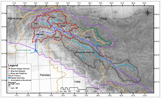
Figure 1.
Upper Indus Basin (UIB): Main catchments, meteorological stations, streams and tributaries.
Climatic variables are usually strongly influenced by topographic altitude. Thus, the northern valley floors of the UIB are arid and warm, with an annual precipitation of only 100–200 mm. These totals increase to 600 mm at 4400 m altitude, and glaciological studies suggest annual accumulation rates of 1500–2000 mm at height of 5500 m [11]. The UIB draws more than 50% of its water from melting of seasonal and permanent snow cover in the Himalaya, Karakoram and the Hindu Kush (HKH) mountains [5,12,13,14,15]. A rise in temperature in the UIB will, therefore, result in elevated melt rates with huge impacts on the timing and magnitude of the generated flows. This will not only lead to a higher average stream flow, but also to an increase in the occurrence and magnitude of extremes, especially during high-precipitation events [16]. There is also the possibility that the peak flows may shift to earlier months or other seasons, with a rise in temperature [5] in the UIB.
All these facts make UIB a very sensitive region to possible climate change, and even, according to some [17], a climate-change “hotspot”. However, despite the necessity of intensified investigations on different aspects of climate change and its possible implications, the task is hindered by the harshness of the environment and the unavailability of representative data. The climatic data available in the UIB lacks suitable coverage, since the in situ meteorological observations in the UIB are sparse and mostly taken at valley stations. Furthermore, the complex orography of the UIB region also affects the amounts, spatial patterns and seasonality of the precipitation. Therefore, neither the sparsely observed station data and gridded data products based on them, nor the sensors-based data, fully represent the precipitation regime of the region [6].
2.2. Data Used
2.2.1. GCM Outputs
In the IPCC 5th assessment report, four representative concentration pathways (RCPs) are normally used as a basis for future climate modelling: one very high baseline emission scenario (RCP8.5), two medium stabilization scenarios (RCP4.5 and RCP6) and one mitigated scenario (RCP2.6) (Table 1).

Table 1.
Representative concentration pathways (RCPs), their radiative forcing, emissions (CO2 equivalent and growth rate %) and temperature increase.
The current study intended to include emission scenarios, covering a wider range of Radiative forcing and future temperature anomaly, while remaining close to the reality and considering RCP’s showing minimum differences with the 2005 onwards actual observed CO2 emission trend and growth rates. Keeping these prerequisites in mind, out of the four options: RCP2.6 was not considered in the current selection as it seemed to be the least likely [18,21] and the mitigation effort implied by this RCP, is unfeasible in the current circumstances [22,23], because it needs a sustained global CO2 mitigation rate of around 3% per year, not a likely prospect, at least in the near future [20].
Out of the remaining three RCPs, the high baseline emission scenario (RCP8.5) and one medium-stabilization scenario (RCP4.5) were selected for the current study. The RCP8.5 was included because it covers the higher end of radiative forcing, as well as the temperature change, and it is also in line with the observed trend of around 3% in the average annual CO2 emission growth rates for 2005–2012 [20,23].
For the medium-stabilization scenarios, both RCP4.5 and RCP6 are equally acceptable, but due to time constraints, and because RCP4.5 shows a better match (≈1.5%) of the trends of the average annual CO2 emission growth rates for the period of 2005–2012 than RCP6 (≈1.0%) [20,23], RCP4.5 was picked along RCP8.5 for the GCM selection procedure.
Additionally, in the current study, only the available GCM runs for the ensemble member r1p1i1 in the CMIP5 repository [24] are included in the initial list. This is done so as to keep open the possibility of using dynamically downscaled projections (driven by the selected GCMs as boundary conditions) by Regional Climate Models (RCMs), which in most cases have utilized boundary conditions from the ensemble member r1p1i1 of the GCMs.
In the current study, a total number of 42 available model runs (ensemble member r1p1i1) are evaluated for RCP4.5 and of 39 for RCP8.5.
2.2.2. Extremes Indices
For the assessment of model runs for extremes, the ETCCDI extremes indices are utilized. The annual extremes of the daily CMIP5 data were acquired from the ETCCDI extremes indices archive [25,26], provided at the “Canadian Centre for Climate Modelling and Analysis”. This data was indirectly obtained and downloaded through the “KNMI Climate Explorer”, which is a web-based research tool to investigate climate and climate change.
2.2.3. Observed Data
The climate station network in the UIB has historically been comprised of only a few low-altitude, valley-based stations. Although the number of in situ observational points has increased since the mid-nineties, with the installations of a few higher altitude automatic weather stations, the coverage is still very thin, and the data is often not very representative, especially for different elevation zones. Similarly, while most of the weather stations have become operational after the mid-nineties, long-term data is a rare commodity and is only available at limited locations.
Similarly, owing to the complex orography of the UIB region and to the co-action of different hydro-climatic regimes, neither the sparse observed station data or the gridded data products based on them, nor the sensor-based climatic datasets fully represent the precipitation regime of the region [6,16,27,28]. Several studies have pointed out that precipitation and other climatic variables in the HKH region exhibit large changes over short distances and considerable vertical gradients [11,29,30,31,32,33,34].
In the absence of long-term climate data with acceptable representation of the UIB climate, most climate-change studies have relied on either the very thin climatic observation network records or the gridded datasets based on them. In all these cases, either the data have acceptable quality, but shorter duration, or they have huge biases, especially, in the case of precipitation in regions with higher altitudes. These biases are further amplified when this data is used as a reference for bias correction or downscaling of climate projections, making the results questionable.
In the current study, therefore, a new long-term climate dataset was prepared (Figure 2). The work related to this new long-term gridded data product [7] is not included in this paper, but we utilized this new dataset instead of the readily available global or regional gridded historical climate datasets, for bias correction, downscaling and assessment of the reliability of climate models for the simulation of the past climate in the region.
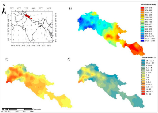
Figure 2.
Reference climate data: (a) Mean annual precipitation (mm), (b) mean temperature- maximum (°C), and (c) mean temperature- minimum (°C).
These gridded precipitation and temperature data are derived, based on all the available in situ observations available in the UIB, through reconstruction for the periods before the mid-nineties, interpolation and correction for the orography and elevation-induced effects guided by available data for runoff, actual evapotranspiration and glacier mass-balance [7].
2.2.4. RCM Outputs
Five CORDEX-SA experiments (Table 6), including IPSL-CM5A-MR_RCA4, MPI-ESM-LR_RCA4, NorESM1-M_RCA4, Can ESM2_RegCM4-4, and GFDL-ESM2M_RCA4, were downscaled and bias corrected. These five GCMs have been dynamically downscaled by CORDEX, using two different RCMs (RCA4 and RegCM4). Their RCM outputs are at considerably finer scale (0.44°) then the source GCMs.
3. Methods
3.1. Selection and Shortlisting of GCMs/RCMs
The full spectrum of GCM projections is wide, with large uncertainties attached [35,36,37], and it cascades to even a larger spectrum when downscaled or translated into possible impacts. Furthermore, the available future projections differ vastly from each other and may range from very wet to drier or very warm to colder future climates, so that the models can be categorized as representing either Warm-Wet, Warm-Dry, Cold-Wet and Cold-Dry corners of the full spectrum, in addition to the projections which are around the median tendency of future model projections.
These issues have led to diverse views on how to select or use these climate model projections, or even whether these climate models or their downscaled outputs should explicitly be used at all, or should only be indirectly used, instead, as guides to generate a range of plausible scenarios more suited for targeted impact studies and practical adaptation planning [38].
In mountainous regions, such as the Upper Indus Basin (UIB), the issue of how to proceed with the climate change impact studies becomes more complicated, because not only may the uncertainties shown by the climate models for these regions be even greater [4,39], but also because of the lower margin for error, as the lives and livelihood of millions of people depend purely on the water resources generated in these basins.
The usual approach of selecting results of a certain model or group of models or opting for a scenario with the mean trend of future projections may not be practical, as the full range of possible future climatic conditions needs to be covered in order to assess the full range of expected impacts required for climate adaptation needs.
As mentioned earlier, the selection of GCMs can be done following different approaches and may be based on a single criterion or a set of criteria. These approaches may include criteria such as: the total amount of change in the mean and/or an extreme of a projected climate variable; the success of a GCM in simulating the past climate for means or extremes; or maybe the skill in presenting the same pattern of tele-connections that drive the climate of the study region, and so on.
The current study adopted a combination of some of these approaches and applied a step-wise shortlisting of climate models based on a range of projected change in the (a) mean, (b) extremes, and (c) skill in reproducing the past climate. As the aim was to arrive at a limited number of models that can represent not only all the possible futures as projected by the entire pool of climate models, but also changes in climatic extremes, so that the selected model runs can provide representation of the full spectrum of future climate projections by GCMs in terms of change in mean, as well as extremes. In other words, for each selected RCP, we intended to filter and select five climate model runs, each representing one the four corners of the spectrum or the median tendencies.
3.1.1. Shortlisting Based on Changes in the Means
As a first step, the total number of available model runs (ensemble member r1p1i1) for RCP4.5 (42) and RCP8.5, (39) were evaluated and shortlisted based on the change presented by them, in terms of the mean annual precipitation sum (ΔP) and the mean air temperature (ΔT), averaged across the UIB, between the simulated reference period historical data (1976–2005) and the late 21st-century projected data (2071–2100). The calculations were done using the web-based application “Climate Explorer” managed by the Royal Netherlands Meteorological Institute (KNMI) (http://climexp.knmi.nl).
As our intention was to identify fewer model runs that best represent the four corners of the full spectrum, as well as the central and middle tendencies, we first determined the 10th, 50th and 90th percentile values of ΔP and ΔT for the entire ensemble considered for each RCP, to explore the extent of the full spectrum of the projected changes in temperature and precipitation under that RCP. This was followed by determining the four (4) closest projections to each of the corners, as well as the center of the spectrum. The total number of shortlisted model runs for each of the two RCPs then amounted to 20.
Details of the different parts of the full spectrum considered during this study are as follows:
- the Dry-Cold corner, represented by the 10th percentile ΔP as well as 10th percentile value of ΔT;
- the Dry-Warm corner, represented by the 10th percentile ΔP but the 90th percentile value of ΔT;
- the Wet-Cold corner, represented by the 90th percentile ΔP and the 10th percentile value of ΔT;
- the Wet-Warm corner, represented by the 90th percentile values for both ΔP as well as ΔT; and finally
- the median projected future climate, represented by the 50th percentile values of both ΔP and ΔT
The identification of the closest model runs to any corner point was done according to the procedure suggested by [19]. It should be noted that 10th and 90th percentiles were selected as the central points of the corners, rather than the maximum or minimum values, in order to avoid selection of any outlier projections.
3.1.2. Ranking Based on Changes in Climate Extremes
To ascertain that preference will be given to those climate model runs that represent the full range of projected change in extremes, all 20 shortlisted model runs for each of RCP4.5 and RCP8.5, were further scrutinized and ranked based on their projected changes in climatic extremes. To that end, the ETCCDI indices [25] (Table 2) were used to evaluate changes in climatic extremes for air temperature, as well as precipitation. For the former, changes in the extremes were ranked and evaluated based on two indices—the warm spell duration index (WSDI), and the cold spell duration index (CSDI)—while for the latter, consecutive dry days (CDD) and the precipitation due to extremely wet days (R99pTOT) were considered.
Table 2.
List of ETCCDI extreme indices used during the GCM selection procedure.
To keep the work manageable, we only analyzed four indices in total, two indices to represent changes in precipitation extremes and two for changes in temperature extremes. Furthermore, as the intended use of the selected climate model ensemble was to force the hydrological model for assessing climate change impacts on both flows and extremes, we chose the four most obvious indicators of precipitation and temperature extremes.
The R99pTOT (precipitation due to extremely wet days (>99th percentile)) and CDD (consecutive dry days: maximum length of dry spell (P < 1 mm)) are appropriate indicators for precipitation extremes and suitable for assessment of associated hydrological extremes. R99pTOT is an important indicator for wet spells in terms of their length and magnitude, which are both key influencing factors in shaping extreme hydrological events (floods and high flows). Similarly, CDD is an important indicator for dry spells that can provide a good opportunity for assessment of the associated low flow episodes. The two temperature-related extreme indices used, i.e., WSDI (count of days in a span of at least 6 days where TX > 90th percentile) and CSDI (count of days in a span of at least 6 days where TN < 10th percentile), seemed best suited for their effects on evapotranspiration and cryospheric processes. The snow and glacier melt/accumulation, as well as evapotranspiration dynamics, are very important in the highly glacierized study area.
The changes in these indices, averaged over the UIB and over 30 years, between the reference period (1976–2005) and the late 21st century projections (2071–2100), were calculated using the database available at the ETCCDI extremes indices archive (http://climexp.knmi.nl), constructed by [26,40].
Only the relevant index for the air temperature or for the precipitation was considered for each of the previously selected group of models (a set of four) initially shortlisted models for each corner or the center), so that for the models in the Wet-Warm corner, only the R99pTOT index for precipitation and the WSDI index for temperature were considered, because they were the only relevant indices, as R99pTOT indicates extreme precipitation events, while WSDI indicates warm spells (Table 2). The other two indices, i.e., CDD and CSDI, were not considered in this case; however, they were the only indices considered for models in the Dry-Cold corner. For each corner, the relevant indices were given scores based on the ratio of the extreme index to the mean of that index, for all four models in a corner. For example, in the Wet-Warm corner, the % change in R99pTOT for a single model is divided by the mean of the % change in R99pTOT for all four models in that corner. The same procedure was applied for WSDI and, finally, both scores were averaged to obtain a final score.
For each of the extreme indices, a weighted rank/skill score (SkEI) was calculated, with the highest value among the group getting the highest weighted rank/skill score of 1, and the others getting a rank according to their difference from this highest value, i.e.,
where Sk is the weighted rank for the specific extreme index EI, h denotes the highest index value in a group, and t denotes the target index to be ranked.
Similarly, in the case of the change in means, i.e., ΔT (°C) and ΔP (%), the ranking (Skm) was done based on the difference ΔT (°C) or ΔP (%) shown by each member with the percentile value relevant to that group,
3.1.3. Ranking Based on Skill in Reproducing the Reference Climate
The models were also evaluated with respect to their skill at simulating the past climate during the reference period (1976–2005). The selected climate model simulations were compared to the reference temperature and the precipitation gridded dataset [7] and were assigned skill scores. We did not use the same method for assigning skill score to temperature and precipitation. For assessing the performance of models in simulating past temperature, the method we applied was adopted from Perkins et al. [41]. In this method, the skill score for temperature is calculated based on the identification of similarities between PDFs of modelled data and the observed reference data. A metric is generated to calculate the cumulative minimum value of each binned value for the two distributions, which represent the common area between two PDFs. This skill score () can be expressed as follows:
where n is the number of bins used to calculate the PDF, ZCM is the frequency of values in a given bin from the model while ZCM is the frequency of values in a given bin from the observed data. This skill score is 1, when there is a perfect match between simulated and the observed data, while a score of 0 means no similarities at all.
The number of bins used in this study to generate the PDFs was 50.
In the case of precipitation, the skill score is calculated by a method proposed by [42] as the product of five skill functions, each assessing similarities between modelled and observed data, while covering different aspects of precipitation behavior. These five skill score functions for a particular model j are listed below:
where ACMj and AObs are the areas below the simulated (climate model j) and the observed precipitation cumulative density function (PDF) curves, respectively, and A+ and A− are the fractional areas over (+) and under (−) the 50th percentile. P denotes the average annual precipitation over UIB and σ is the standard deviation of the probability distribution function.
Each of the above factors is intended to cover different aspects of probability distribution characteristics of the climate models, so that the distribution as a whole is taken into account through the mean and the total area (Equations (4) and (7)), the smaller and higher precipitation amounts are accounted for, through the 50th-percentile limit (Equations (5) and (6)), while the shape of the distribution is defined through the variance (Equation (8)).
These five factors are multiplied together to yield a single final skill score (SkPrec) for precipitation estimated by each model j:
As a final step, all the rankings/scores, based on the changes in the means and in the extremes, as well as the skill scores for reproducing reference temperature and precipitation, are multiplied together to get the final overall skill or rank as follows:
Under this skill score, a higher value indicates better performance, while a lower value indicates otherwise. These skill scores can be further translated to a simple ranking of 1 to 4 for each group of climate models.
The climate model selection procedure adopted in this study is in line with the approach and methods suggested by [21,41,42], although with certain modifications in the evaluation criteria. For assessing the performance of models in simulating past temperature, the method applied is adopted from [41], while in the case of precipitation, guidance is taken from [42]. A major difference from [21] in assessing model performances in simulating past climate is the use of a new long-term climate data set and an additional evaluation step for assessing model runs for their skill in reproducing the annual cycle of precipitation and temperature as well.
3.2. Downscaling and Bias Correction
After the shortlisting and ranking of the GCMs, the next step was to address the two primary issues inhibiting impact studies: firstly, the coarse spatial scales represented by the GCM may not be as fine as required by regional- and local-scale environmental modelling or impact studies; and secondly, the GCM raw outputs, or their downscaled versions, are deemed to contain systematic errors (bias) of certain magnitude, relative to the observational data, and therefore need post-processing by correcting it with and towards observations prior their its use in environmental modelling or impact studies.
The downscaling can be done either by applying statistical downscaling methods or through dynamical downscaling via application of a regional climate model (RCM). As dynamical downscaling was too demanding in terms of time and computational resource requirements, we decided only to explore whether any dynamically downscaled RCM projections were available for the already shortlisted and ranked GCMs. The Coordinated Regional Downscaling Experiment (CORDEX) has generated fine-scale climate projections for different regions of the world, of which the CORDEX-South Asia experiments cover the UIB region. We found that CORDEX-RCM model projections were available for four of the selected GCMs at the 1st rank and one GCM at the 2nd rank. These RCM projections provide dynamically downscaled data at a resolution of ~ 50 km for all of our selected GCMs. The data for the relevant GCM–RCM combinations were downloaded, but needed further downscaling, as the scale was still not fine enough, and also needed to undergo bias correction before further use in hydrological modelling.
This downscaling and bias correction was achieved by the Distribution Mapping method (DM) [43], which was selected out of five different bias correction methods for the precipitation climate variable. These methods included: (1) Linear Scaling (LS); (2) Local Intensity Scaling (LIS); (3) Power Transformation (PT); (4) Distribution Mapping (DM); and (5) Distribution Mapping followed by Intensity and frequency Scaling (DM-IS).
For the temperature, the selection was made after evaluating the performance of the following three bias correction methods: (1) Linear Scaling (LS); (2) Variance Scaling (VS); and (3) Distribution Mapping (DM). Further details of these methods can be found in [43].
The calibration and validation statistics, along with brief explanations, are provided as appendices (Supplementary Materials: Appendix A, Tables A1 and A2).
4. Results
4.1. Selection of Climate Models
4.1.1. Shortlisting of Models: Changes in Climatic Means
The results of the initial shortlisting of the GCM model runs are given in Figure 3 and Figure 4. In this step, only those GCM runs were retained which showed minimal difference with the 10th, 50th and 90th percentile values of ΔT (°C) and ΔP (%), so that, for each RCP, we were left with sets of 4 GCM runs at each corner and 4 in the middle, while the remaining model runs were not processed any further. In this way, a total of 20 model runs were selected for each RCP.
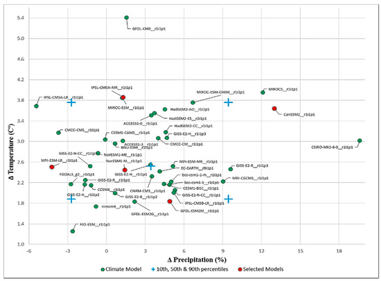
Figure 3.
Projected changes in mean air temperature (ΔT) and annual precipitation sum (ΔP) between 2071 and 2100 and 1971 and 2000 for all included RCP4.5 GCM runs. Blue crosses indicate the 10th, 50th and 90th percentile values for ΔT and ΔP. The model runs shortlisted during this step are indicated in red color.
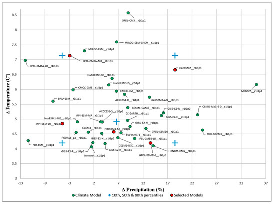
Figure 4.
Similar to Figure 3, but for RCP8.5 GCM runs.
It is worth mentioning that the range of projections for ΔT and ΔP for the RCP8.5 model pool was much larger than for the RCP4.5 model pool. For the latter, more extreme RCP, ΔP ranges from −5.42% to 19.56%, and ΔT ranges from 1.26 °C to 5.41 °C; while for the former (RCP4.5), these ranges are much higher, with ΔP ranging between −12.01% and 35.12% and ΔT between 1.48 °C and 8.57 °C.
The shortlisted GCM runs were also ranked according to their differences with the 10th, 50th or 90th percentile values in the respective corner or center. This ranking was intended for use in the final selection step, so that those model runs which show closest representation of the group of models or type of scenarios (Warm-Wet, Warm-Dry, Cold-Wet, Cold-Dry or the Median) get preference during the final selection.
It should be noted that the term Cold used in the “Wet-Cold” and “Dry-Cold” scenarios does not mean that the future temperatures will be colder than those of the reference period, but rather indicates that the warming will be less than that of the Warm scenarios. Similarly, the term Dry in the scenarios “Dry-Cold”and “Dry-Warm” is also only indicative of its comparative position relative to other climate models.
4.1.2. Ranking Based on Changes in Climatic Extremes
The 20 shortlisted model runs for each RCP were further scrutinized based on their projected changes in climatic extremes. The details of the projected changes in selected extreme indices are given in Table 3. The darker colors indicate the higher values, while the lighter indicates lower values. These indices were given a weighted rank/score based on their difference from the highest value in the group of four model runs in a corner.
Table 3.
Percentage change in ETCCDI indices (R99pTOT, CDD, WSDI, and CSDI) along with changes in mean precipitation (ΔP) and temperature (ΔT), for all corners/scenarios (Warm-Wet, Warm-Dry, Cold-Wet and Cold-Dry) and both RCPs (RCP4.5 and RCP8.5).
Similar to the rank assigned based on changes in the means, this ranking was also intended for use in the final selection step, so that the model runs, which show the largest changes in the extreme indices for each of the corner: Warm-Wet, Warm-Dry, Cold-Wet or Cold-Dry, get preference during the final selection. Unlike the four corners, evaluation based on the extreme indices was not carried out for the central or the mean scenario.
The ranking and scores for means and extreme indices, as well as the skill scores for simulating reference climate, are presented in Table 4 and Table 5 for RCP4.5 and RCP8.5, respectively.
Table 4.
Weighted ranks for all shortlisted RCP4.5 GCM runs based on change in means (e and f), change in extremes (a, b, c and d) and their skill scores for simulating reference precipitation and air temperature(g and h).
Table 5.
Similar to Table 4, but for RCP8.5.
In most cases, the model run with the highest or the lowest changes in mean precipitation or temperature coincide with the highest change in relevant extreme index as well.
The index Δ R99pTOT (%) was evaluated to represent the “Wet” scenarios, while the Δ CDD (%) represented the “Dry” scenarios. Similarly, Δ WSDI (%) was considered for the “Warm” scenarios, while Δ CSDI (%) was considered for the “Cold” scenarios. In this way, a set of two (2) indices out of the four (4) were evaluated for each of the scenarios: Warm-Wet, Warm-Dry, Cold-Wet, and Cold-Dry.
4.1.3. Ranking Based on Skill in Reproducing the Reference Climate
After checking the model runs for their projected changes in means and extreme indices, they were finally evaluated for their skill at reproducing the reference precipitation and temperature data.
The ranking for past performance utilized a new set of reference precipitation and temperature data [7], averaged over the UIB. The skill scores were calculated following the procedure of Section 4.1.3, and are presented in columns g and h in Table 4 and Table 5. For most scenarios, the same models performed better than the others for both RCPs in simulating past climate.
After allocating the skill score based on the past performance, the final skill scores and ranks were calculated by multiplying all the relevant skill scores allocated to each model run. The final ranks were allocated to each scenario, with the highest rank allotted to the model run with highest final skill score, and so on.
It is interesting to note that for the 4 scenarios, Warm-Dry, Cold-Wet, Cold-Dry and Median, for both RCPs, the same GCMs get the highest skill scores and ranks. The only exception is the Warm-Wet scenario, where different models top the ranking. In this scenario, for RCP4.5, the GCM “MIROC5” is in the top rank, followed by “CanESM2”, while for RCP8.5, the ranking of these two GCMs is reversed.
4.1.4. Limitations of the Model Selection Procedure
In the previous section, the step-wise shortlisting of the various climate models was based on the range of projected change in (a) mean, (b) extremes, and (c) skill in reproducing the past climate. Although the main aim of this approach was to combine the strengths of two different methodologies, i.e., the selection of the GCMs based on the properties of the full range of projections and the selection procedures based on past performance, certain limitations are unavoidable and need to be discussed.
First of all, the analysis considered only models selected based on the changes in the means and only the ensemble member r1p1i1, resulting in a reduced number of GCM runs for evaluation and possibly a smaller range of climatic extremes. This may also have led to possibly screening out models which may have had better past performance.
Similarly, another issue is concerned with the scale at which the method was applied. During the shortlisting step, and also during the evaluation of extreme indices, the projected changes or ETCCDI extremes indices were averaged over the entire UIB, which has the possibility of decreasing the spatial variation in projected changes.
Additionally, the weighting of different skill scores in this study also differed for similar work, such as [21]. In our study, the final skill score was a combination of scores allocated for change in mean, change in extremes, and performance in reproducing past climate. This may have reduced the chances of selecting the climate model with the best past performance, but increased the chance of a better spread of scenarios over the entire range, while still taking past performance as a key factor in selections. Our model selection approach also assumes that all the evaluated model runs are independent of each other, which may not be the case, as some models use the same forcing and validation data or may share similar model codes [44,45].
Despite these limitations, the adopted approach made it possible for us to identify a limited number of model runs, representative of the full range of future projected means and extremes while giving due preference to models which perform better at simulating the reference climate.
4.2. Bias Correction and Downscaling of Future Climate Scenarios
The future climate projections of the selected climate models needed to be downscaled and corrected for biases, before further use in hydrological model simulation. Therefore, as a first option, all the dynamically downscaled climate projections available for UIB were checked for whether any Regional Climate Model (RCM) projections were available that have dynamically downscaled projections for the already shortlisted GCM at first or second position in the ranking. We found that, for both RCPs, the outputs of at least three (3) CORDEX-SA experiments were based on the GCMs ranked 1st in our study (IPSL-CM5A-MR_RCA4, MPI-ESM-LR_RCA4 and NorESM1-M_RCA4). The GSM CanESM2, which is at 2nd rank for RCP4.5 and at 1st for RCP8.5, has dynamically downscaled projections under CORDEX-SA experiments, CanESM2_RegCM4-4. The output of one CORDEX-SA experiment (GFDL-ESM2M_RCA4) was based on GFDL-ESM2M, which is ranked at 2nd position for both the RCPs in our study (Table 4 and Table 5).
It was decided to utilize the available dynamically downscaled data for our selected GCMs, ranked at 1st or 2nd positions. Therefore, five CORDEX-SA experiments (Table 6), including IPSL-CM5A-MR_RCA4, MPI-ESM-LR_RCA4, NorESM1-M_RCA4, Can ESM2_RegCM4-4, and GFDL-ESM2M_RCA4 were selected for further processing and bias correction. These five GCMs were dynamically downscaled by CORDEX using two different RCMs (RCA4 and RegCM4). Their RCM outputs are at a considerably finer scale (0.44°) than the source GCMs.
Table 6.
List of CORDEX South Asia experiments for RCP8.5 and their CMIP5-GCM forcing.
4.3. Projected Changes in Temperature and Precipitation
The five (5) selected (CORDEX-SA) RCM outputs were further bias-corrected using the “distribution mapping technique” [43] for RCP4.5 and RCP8.5 for two sets of durations, i.e., mid-century (2041–2070) and end-century (2071–2100). Major properties of the downscaled projections are given in Table 7.
Table 7.
Future precipitation and temperature projections from 5 GCM models, 2 RCPs and 2 periods.
The downscaled projections show changes in temperature ranging from 2.3 °C to 6.33 °C for RCP4.5 and of 2.92 °C to 9.0 °C for RCP8.5. The downscaled and bias-corrected precipitation ranges from a minor increase of 2.2% for the drier scenarios to as high as 15.9% for the wet scenarios. Thus, both temperature and precipitation show increases, as do the extremes, since the probabilities of the wet days are projected to decrease, while the precipitation intensities are projected to increase unanimously by both RCPs.
The spatial distribution of the projected future changes for precipitation and temperature across the UIB also show certain distinct trends. Thus, the precipitation (Figure 5) over the mid-century (2041–2070), as well as the late century (2071–2100), reveals for all scenarios a remarkable decrease in the southeastern parts of the basin, but an increase in the northeastern parts. This decrease/increase is particularly intense for the “Dry-Warm” and the “Median” scenarios over the late 21st century.
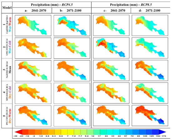
Figure 5.
Spatial distribution of projected precipitation change across the UIB over the mid (2014–2070) and the late- (2071–2100) 21st century for 5 models and 2 RCPs. The figure is arranged in a tabular form where the 1st and 2nd column represent projected change in precipitation for RCP 4.5, for the mid-century (2014–2070) and the late-century (2071–2100), respectively, while the 3rd and 4th columns show the projected change in the mid-century and the late-century precipitation for RCP 8.5, respectively. The rows represent the climate models used.
The spatial distribution of the projected changes for in temperature (Figure 6) also shows similarities across all scenarios, with the northern and northwestern parts of the basin exhibiting higher increases, while the eastern and southern parts experience a comparatively smaller temperature increase.
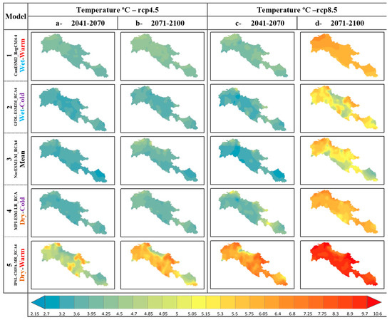
Figure 6.
Similar to Figure 5, but for temperature changes.
For RCP8.5, the projected temperature changes appear to be very high over the late 21st century and this occurs under all scenarios, especially for the “Warm” scenarios, with an almost uniform spread across the whole UIB. The projected temperature changes range for all RCPs and the two 20th-century periods from a minimum increase of 3.76 °C (NorESM1-M_RCA4, RCP4.5, Period: 2041–2070) to a maximum increase as high as 10.4 °C (IPSL-CM5A-MR_RCA4, RCP8.5 and period: 2071–2100).
4.4. Limitations of the Downscaling and Bias Correction Approach Adopted
The downscaling and bias correction approaches described in the previous sections, although adopted as the best available option considering the availability of time, resources and data, are still not without limitations.
Firstly, we opted for using GCM-RCM chains for the already shortlisted climate model runs where the RCM add further detail to global climate simulations and may provide regional- to local-scale information, but their outputs are still subject to inherited or new systematic errors and may therefore require a bias correction or further downscaling to a higher resolution, along with the fact that they may also produce quite a different response in terms of the temperature and precipitation change than the forcing GCMs. In fact, many authors recognized this affliction of GCM-RCM model chains with systematic errors (biases) [48,49,50,51,52,53,54,55], but still the representation of explicit atmospheric and surface processes and the level of spatial details provided by the RCMs [56] make them a better option for regions with high topographic variability, The selection procedure may in future, though, directly include the RCM runs instead of GCM, when an appropriate amount of RCM runs are available.
The systematic errors (biases) in GCM/RCM outputs make them unsuitable for certain uses, and application of different bias-correction methods has increasingly become a standard procedure, especially in climate change impact studies [57].
Although these bias correction approaches improve the agreement of climate model output with observations, and therefore narrows the uncertainty range of predictions and simulations, they do so without a sound physical basis [57]. At the same time, a growing number of authors are showing reservations on the use of bias correction methods for a variety of reasons. Some argue that the main assumption behind bias correction approaches is the stationarity of the correction parameters, which is not realistic and may not be the case, especially under climate change [57,58]. While others believe that as bias correction cannot overcome major climate model errors, inexperienced application might result in ill-informed adaptation decisions [59]. Despite being critical of bias correction methods, many of these authors e.g., [57,59,60] acknowledge the need for some type of bias correction and recommend different precautions to avoid any pitfalls.
5. Conclusions
It is essential to have representative future climate projections of appropriate quality for climate change impact studies, especially in the water resource sector. Despite the availability of an increasing number of GCM outputs in the CMIP5 archive and the on-going improvements in their process representations, issues of large uncertainties in their future climate predictions cannot be avoided. This situation, along with other factors, such as time, human resources or computational constraints, make it imperative to sort out the most appropriate individual GCM or small ensemble of GCMs for a more reliable assessment of climate change impacts.
The approach presented in the present study seeks the most suitable set of climate model runs, while considering not only the full ranges of projected changes in terms of means and extremes by different climate models, but also their skills in simulating the past climate in a reference period.
This selection procedure was applied for future climate projections over the Upper Indus Basin for two representative concentration pathways (RCPs), the RCP 4.5 and RCP 8.5. All available model runs for the r1p1i1 ensemble member of each GCM in the CMIP5 repository were included in the initial list. The total number of model runs available for RCP4.5 was 42, and 39 for RCP8.5.
Based on the huge uncertainties reported in the GCM runs for the UIB, all possible extreme future scenarios (Wet-Warm, Wet-Cold, Dry-Warm, Dry-Cold) were considered, in addition to the selection of GCMs representing the mean future climate change, with respect to both changes in the projected means and the extremes. This procedure made it possible to arrive at a limited number of climate models, from which the final selection was performed by assigning ranks based on the weighted score for each of the mentioned selection criteria.
Finally, the precipitation and temperature time series of the selected GCM model runs were bias corrected and further downscaled to the scale of the reference data by means of a distribution mapping technique. The ensembles of the selected GCM runs for RCP4.5 and RCP8.5 scenarios show that the uncertainty of future climate in the study region is very large for the raw data, as well as their downscaled versions.
The downscaled projections indicate increases of temperature ranging between 2.3 °C and 9.0 °C and changes in precipitation that range from a slight annual increase of 2.2% under the drier scenarios, to as high as 15.9% for the wet scenarios. Thus, for both temperature and precipitation, the future projections under all scenarios and both RCP’s only show increases in the mean annual values, with no negative trend. Moreover, for all scenarios, the future precipitation is projected to be more extreme, as the probability of wet days decreases, while at the same time, the precipitation intensities will increase.
The spatial distribution of the downscaled predictors, namely, the precipitation, also shows distinct patterns across the UIB, such that this variable shows for all time periods/scenarios considered a distinct decrease in the southeastern parts, but an increase in the northeastern parts of the basin. This decrease/increase is particularly intense for the “Dry-Warm” and the “Median” scenarios over the late 21st century.
Overall, the future climate of the UIB region remains very uncertain, which justifies the selection procedure proposed here to arrive at a wider range of possible climate scenarios that can then be further utilized and translated into a wider spectrum of climate change impact scenarios.
Supplementary Materials
The following are available online at http://www.mdpi.com/2225-1154/6/4/89/s1.
Author Contributions
Conceptualization, A.J.K.; Formal analysis, A.J.K.; Investigation, A.J.K.; Methodology, A.J.K.; Resources, M.K.; Supervision, M.K.; Validation, A.J.K.; Writing—original draft, A.J.K.; Writing—review & editing, M.K.
Funding
This research received no external funding.
Acknowledgments
We acknowledge provision of data by the following sources:
- The data sets for changes in mean/extremes were acquired from “KNMI Climate Explorer”, web application to analysis climate data statistically. It is part of the WMO Regional Climate Centre at KNMI, Netherland;
- CORDEX-South Asia experiment, RCMs data, hosted at Centre for Climate Change Research (CCCR) at the Indian Institute of Tropical Meteorology (IITM).
Conflicts of Interest
The authors declare no conflict of interest.
References
- Biemans, H.; Speelman, L.H.; Ludwig, F.; Moors, E.J.; Wiltshire, A.J.; Kumar, P.; Gerten, D.; Kabat, P. Future water resources for food production in five South Asian river basins and potential for adaptation—A modeling study. Sci. Total Environ. 2013, 468, S117–S131. [Google Scholar] [CrossRef] [PubMed]
- Pierce, D.W.; Barnett, T.P.; Santer, B.D.; Gleckler, P.J. Selecting global climate models for regional climate change studies. Proc. Natl. Acad. Sci. USA 2009, 106, 8441–8446. [Google Scholar] [CrossRef] [PubMed]
- Turner, A.G.; Annamalai, H. Climate change and the South Asian summer monsoon. Nat. Clim. Chang. 2012, 2, 587–595. [Google Scholar] [CrossRef]
- Mishra, V. Climatic uncertainty in Himalayan water towers. J. Geophys. Res. Atmos. 2015, 120, 2689–2705. [Google Scholar] [CrossRef]
- Lutz, A.F.; Immerzeel, W.W.; Kraaijenbrink, P.D.A.; Shrestha, A.B.; Bierkens, M.F.P. Climate Change Impacts on the Upper Indus Hydrology: Sources, Shifts and Extremes. PLoS ONE 2016, 11, e0165630. [Google Scholar] [CrossRef] [PubMed]
- Palazzi, E.; Hardenberg, J.; von Provenzale, A. Precipitation in the Hindu-Kush Karakoram Himalaya: Observations and future scenarios. J. Geophys. Res. Atmos. 2013, 118, 85–100. [Google Scholar] [CrossRef]
- Khan, A.J.; Koch, M. Correction and Informed Regionalization of Precipitation Data in a High Mountainous Region (Upper Indus Basin) and Its Effect on SWAT-Modelled Discharge. Water 2018, 10, 1557. [Google Scholar] [CrossRef]
- De-Souza, K.; Kituyi, E.; Harvey, B.; Leone, M.; Murali, K.S.; Ford, J.D. Vulnerability to climate change in three hot spots in Africa and Asia: Key issues for policy-relevant adaptation and resilience-building research. Reg. Environ. Chang. 2015, 15, 747–753. [Google Scholar] [CrossRef]
- Nepal, S.; Shrestha, A.B. Impact of climate change on the hydrological regime of the Indus, Ganges and Brahmaputra river basins: A review of the literature. Int. J. Water Resour. Dev. 2015, 31, 201–218. [Google Scholar] [CrossRef]
- Arnold, J.G.; Srinivasan, R.; Muttiah, R.S.; Williams, J.R. Large area hydrologic modeling and assessment part I: Model development. J. Am. Water Resour. Assoc. 1998, 34, 73–89. [Google Scholar] [CrossRef]
- Wake, C.P. Glaciochemical Investigations as a Tool for Determining the Spatial and Seasonal Variation of Snow Accumulation in the Central Karakoram, Northern Pakistan. Ann. Glaciol. 1989, 13, 279–284. [Google Scholar] [CrossRef]
- Tahir, A.A.; Chevallier, P.; Arnaud, Y.; Ahmad, B. Snow cover dynamics and hydrological regime of the Hunza River basin, Karakoram Range, Northern Pakistan. Hydrol. Earth Syst. Sci. 2011, 15, 2275–2290. [Google Scholar] [CrossRef]
- Ali, K.F.; de Boer, D.H. Spatial patterns and variation of suspended sediment yield in the upper Indus River basin, northern Pakistan. J. Hydrol. 2007, 334, 368–387. [Google Scholar] [CrossRef]
- Archer, D. Contrasting hydrological regimes in the upper Indus Basin. J. Hydrol. 2003, 274, 198–210. [Google Scholar] [CrossRef]
- Immerzeel, W.W.; van Beek, L.P.H.; Bierkens, M.F.P. Climate Change Will Affect the Asian Water Towers. Science 2010, 328, 1382–1385. [Google Scholar] [CrossRef] [PubMed]
- Wijngaard, R.R.; Lutz, A.F.; Nepal, S.; Khanal, S.; Pradhananga, S.; Shrestha, A.B.; Immerzeel, W.W. Future changes in hydro-climatic extremes in the Upper Indus, Ganges, and Brahmaputra River basins. PLoS ONE 2017, 12, e0190224. [Google Scholar] [CrossRef] [PubMed]
- Kilroy, G. A review of the biophysical impacts of climate change in three hotspot regions in Africa and Asia. Reg. Environ. Chang. 2015, 15, 771–782. [Google Scholar] [CrossRef]
- Van Vuuren, D.P.; Edmonds, J.; Kainuma, M.; Riahi, K.; Thomson, A.; Hibbard, K.; Hurtt, G.C.; Kram, T.; Krey, V.; Lamarque, J.-F.; et al. The representative concentration pathways: An overview. Clim. Chang. 2011, 109, 5–31. [Google Scholar] [CrossRef]
- Wayne, G.P. The Beginner’s Guide to Representative Concentration Pathways. Available online: https://www.skepticalscience.com/docs/RCP_Guide.pdf (accessed on 1 January 2018).
- Peters, G.P.; Andrew, R.M.; Boden, T.; Canadell, J.G.; Ciais, P.; Le Quéré, C.; Marland, G.; Raupach, M.R.; Wilson, C. The challenge to keep global warming below 2 °C. Nat. Clim. Chang. 2013, 3, 4–6. [Google Scholar] [CrossRef]
- Lutz, A.F.; ter Maat, H.W.; Biemans, H.; Shrestha, A.B.; Wester, P.; Immerzeel, W.W. Selecting representative climate models for climate change impact studies: An advanced envelope-based selection approach. Int. J. Climatol. 2016, 36, 3988–4005. [Google Scholar] [CrossRef]
- Mora, C.; Frazier, A.G.; Longman, R.J.; Dacks, R.S.; Walton, M.M.; Tong, E.J.; Sanchez, J.J.; Kaiser, L.R.; Stender, Y.O.; Anderson, J.M.; et al. The projected timing of climate departure from recent variability. Nature 2013, 502, 183–187. [Google Scholar] [CrossRef] [PubMed]
- Sanford, T.; Frumhoff, P.C.; Luers, A.; Gulledge, J. The climate policy narrative for a dangerously warming world. Nat. Clim. Chang. 2014, 4, 164–166. [Google Scholar] [CrossRef]
- Taylor, K.E.; Stouffer, R.J.; Meehl, G.A. An Overview of CMIP5 and the Experiment Design. Bull. Am. Meteorol. Soc. 2012, 93, 485–498. [Google Scholar] [CrossRef]
- Peterson, T.C. Climate change indices. WMO Bull. 2005, 54, 83–86. [Google Scholar]
- Sillmann, J.; Kharin, V.V.; Zhang, X.; Zwiers, F.W.; Bronaugh, D. Climate extremes indices in the CMIP5 multimodel ensemble: Part 1. Model evaluation in the present climate. J. Geophys. Res. Atmos. 2013, 118, 1716–1733. [Google Scholar] [CrossRef]
- Yatagai, A.; Kamiguchi, K.; Arakawa, O.; Hamada, A.; Yasutomi, N.; Kitoh, A. APHRODITE: Constructing a Long-Term Daily Gridded Precipitation Dataset for Asia Based on a Dense Network of Rain Gauges. Bull. Am. Meteorol. Soc. 2012, 93, 1401–1415. [Google Scholar] [CrossRef]
- Palazzi, E.; Filippi, L.; von Hardenberg, J. Insights into elevation-dependent warming in the Tibetan Plateau-Himalayas from CMIP5 model simulations. Clim. Dyn. 2017, 48, 3991–4008. [Google Scholar] [CrossRef]
- Dahri, Z.H.; Ludwig, F.; Moors, E.; Ahmad, B.; Khan, A.; Kabat, P. An appraisal of precipitation distribution in the high-altitude catchments of the Indus basin. Sci. Total Environ. 2016, 548, 289–306. [Google Scholar] [CrossRef] [PubMed]
- Pang, H.; Hou, S.; Kaspari, S.; Mayewski, P.A. Influence of regional precipitation patterns on stable isotopes in ice cores from the central Himalayas. Cryosphere 2014, 8, 289–301. [Google Scholar] [CrossRef]
- Hewitt, K. Glacier Change, Concentration, and Elevation Effects in the Karakoram Himalaya, Upper Indus Basin. Mt. Res. Dev. 2011, 31, 188–200. [Google Scholar] [CrossRef]
- Winiger, M.; Gumpert, M.; Yamout, H. Karakorum-Hindukush-western Himalaya: Assessing high-altitude water resources. Hydrol. Process. 2005, 19, 2329–2338. [Google Scholar] [CrossRef]
- Weiers, S. Zur Klimatologie des NW-Karakorum und Angrenzender Gebiete. Statistische Analysen Unter Einbeziehung von Wettersatellitenbildern und Eines Geographischen Informationssystems (GIS); Kommission bei F. Dümmler: Bonn, Germany, 1995. [Google Scholar]
- Dhar, O.N.; Rakhecha, P.R. The Effect of Elevation on Monsoon Rainfall Distribution in the Central Himalayas. In Monsoon Dynamics; Lighthill, M.J., Pearce, R.P., Eds.; Cambridge University Press: New York, NY, USA, 1981; pp. 253–260. [Google Scholar]
- Wilby, R.L.; Dawson, C.W.; Murphy, C.; O’Connor, P.; Hawkins, E. The Statistical DownScaling Model-Decision Centric (SDSM-DC): Conceptual basis and applications. Clim. Res. 2014, 61, 259–276. [Google Scholar] [CrossRef]
- Pielke, R.A.; Wilby, R.L. Regional climate downscaling: What’s the point? Eos Trans. Am. Geophys. Union 2012, 93, 52–53. [Google Scholar] [CrossRef]
- Stakhiv, E.Z. Pragmatic Approaches for Water Management Under Climate Change Uncertainty1. J. Am. Water Resour. Assoc. 2011, 47, 1183–1196. [Google Scholar] [CrossRef]
- Wilby, R.L.; Dessai, S. Robust adaptation to climate change. Weather 2010, 65, 180–185. [Google Scholar] [CrossRef]
- Sanjay, J.; Krishnan, R.; Shrestha, A.B.; Rajbhandari, R.; Ren, G.-Y. Downscaled climate change projections for the Hindu Kush Himalayan region using CORDEX South Asia regional climate models. Adv. Clim. Chang. Res. 2017, 8, 185–198. [Google Scholar] [CrossRef]
- Sillmann, J.; Kharin, V.V.; Zwiers, F.W.; Zhang, X.; Bronaugh, D. Climate extremes indices in the CMIP5 multimodel ensemble: Part 2. Future climate projections. J. Geophys. Res. Atmos. 2013, 118, 2473–2493. [Google Scholar] [CrossRef]
- Perkins, S.E.; Pitman, A.J.; Holbrook, N.J.; McAneney, J. Evaluation of the AR4 Climate Models’ Simulated Daily Maximum Temperature, Minimum Temperature, and Precipitation over Australia Using Probability Density Functions. J. Clim. 2007, 20, 4356–4376. [Google Scholar] [CrossRef]
- Sánchez, E.; Romera, R.; Gaertner, M.A.; Gallardo, C.; Castro, M. A weighting proposal for an ensemble of regional climate models over Europe driven by 1961–2000 ERA40 based on monthly precipitation probability density functions. Atmos. Sci. Lett. 2009, 10, 241–248. [Google Scholar] [CrossRef]
- Teutschbein, C.; Seibert, J. Bias correction of regional climate model simulations for hydrological climate-change impact studies: Review and evaluation of different methods. J. Hydrol. 2012, 456, 12–29. [Google Scholar] [CrossRef]
- Knutti, R.; Masson, D.; Gettelman, A. Climate model genealogy: Generation CMIP5 and how we got there. Geophys. Res. Lett. 2013, 40, 1194–1199. [Google Scholar] [CrossRef]
- Jun, M.; Knutti, R.; Nychka, D.W. Local eigenvalue analysis of CMIP3 climate model errors. Tellus A Dyn. Meteorol. Oceanogr. 2008, 60, 992–1000. [Google Scholar] [CrossRef]
- Giorgi, F.; Coppola, E.; Solmon, F.; Mariotti, L.; Sylla, M.B.; Bi, X.; Elguindi, N.; Diro, G.T.; Nair, V.; Giuliani, G.; et al. RegCM4: Model description and preliminary tests over multiple CORDEX domains. Clim. Res. 2012, 52, 7–29. [Google Scholar] [CrossRef]
- Samuelsson, P.; Jones, C.G.; Will´En, U.; Ullerstig, A.; Gollvik, S.; Hansson, U.; Jansson, E.; Kjellstro, M.C.; Nikulin, G.; Wyser, K. The Rossby Centre Regional Climate model RCA3: Model description and performance. Tellus A Dyn. Meteorol. Oceanogr. 2011, 63, 4–23. [Google Scholar] [CrossRef]
- Wilby, R.L.; Hay, L.E.; Gutowski, W.J.; Arritt, R.W.; Takle, E.S.; Pan, Z.T.; Leavesley, G.H.; Clark, M.P. Hydrological responses to dynamically and statistically downscaled climate model output. Geophys. Res. Lett. 2000, 27, 1199–1202. [Google Scholar] [CrossRef]
- Wood, A.W.; Leung, L.R.; Sridhar, V.; Lettenmaier, D.P. Hydrologic implications of dynamical and statistical approaches to downscaling climate model outputs. Clim. Chang. 2004, 62, 189–216. [Google Scholar] [CrossRef]
- Randall, D.A.; Wood, R.A.; Bony, S.; Colman, R.; Fichefet, T.; Fyfe, J.; Kattsov, V.; Pitman, A.; Shukla, J.; Srinivasan, J.; et al. Climate Models and Their Evaluation. In Climate Change 2007: The Physical Science Basis; Contribution of Working Group I to the Fourth Assessment Report of the Intergovernmental Panel on Climate Change; Cambridge University Press: Cambridge, UK; New York, NY, USA, 2007. [Google Scholar]
- Piani, C.; Weedon, G.P.; Best, M.; Gomes, S.M.; Viterbo, P.; Hagemann, S.; Haerter, J.O. Statistical bias correction of global simulated daily precipitation and temperature for the application of hydrological models. J. Hydrol. 2010, 395, 199–215. [Google Scholar] [CrossRef]
- Hagemann, S.; Chen, C.; Haerter, J.O.; Heinke, J.; Gerten, D.; Piani, C. Impact of a sta25 tistical bias correction on the projected hydrological changes obtained from three GCMs and two hydrology models. J. Hydrometeorol. 2016, 12, 556–578. [Google Scholar] [CrossRef]
- Chen, C.; Haerter, J.O.; Hagemann, S.; Piani, C. On the contribution of statistical bias correction to the uncertainty in the projected hydrological cycle, Geophys. Res. Lett. 2011, 38, L20403. [Google Scholar] [CrossRef]
- Rojas, R.; Feyen, L.; Dosio, A.; Bavera, D. Improving pan-European hydrological simulation of extreme events through statistical bias correction of RCM-driven climate simulations. Hydrol. Earth Syst. Sci. 2011, 15, 2599–2620. [Google Scholar] [CrossRef]
- Haddeland, I.; Heinke, J.; Voß, F.; Eisner, S.; Chen, C.; Hagemann, S.; Ludwig, F. Effects of climate model radiation, humidity and wind estimates on hydrological simulations. Hydrol. Earth Syst. Sci. 2012, 16, 305–318. [Google Scholar] [CrossRef]
- Trzaska, S.; Schnarr, E.; A Review of Downscaling Methods for Climate Change Projections. United States Agency for International Development (USAID) under the African and Latin American Resilience to Climate Change (ARCC) Project by Tetra Tech ARD, Burlington, Vermont, USA. 2014, pp. 1–42. Available online: http://www.ciesin.org/documents/Downscaling_CLEARED_000.pdf (accessed on 1 January 2018).
- Ehret, U.; Zehe, E.; Wulfmeyer, V.; Warrach-Sagi, K.; Liebert, J. “HESS Opinions” Should we apply bias correction to global and regional climate model data? Hydrol. Earth Syst. Sci. 2012, 16, 3391–3404. [Google Scholar] [CrossRef]
- Vannitsem, S. Bias correction and post-processing under climate change. Nonlinear Process. Geophys. 2011, 18, 911–924. [Google Scholar] [CrossRef]
- Maraun, D.; Shepherd, T.G.; Widmann, M.; Zappa, G.; Walton, D.; Gutiérrez, J.M.; Hagemann, S.; Richter, I.; Soares, P.M.; Hall, A.; Mearns, L.O. Towards process-informed bias correction of climate change simulations. Nat. Clim. Chang. 2017, 7, 764. [Google Scholar] [CrossRef]
- Maraun, D. Bias correcting climate change simulations-a critical review. Curr. Clim. Chang. Rep. 2016, 2, 211–220. [Google Scholar] [CrossRef]
© 2018 by the authors. Licensee MDPI, Basel, Switzerland. This article is an open access article distributed under the terms and conditions of the Creative Commons Attribution (CC BY) license (http://creativecommons.org/licenses/by/4.0/).