

Preliminary Feasibility Study of the Ad Hoc Separation Operational Concept
by
 , , , ,
Lidia Serrano-Mira
1,* ,
,
Luis Pérez Sanz
1 ,
,
Javier A. Pérez-Castán
1,
Fedja Netjasov
2,
Irene García Moreno
1 and
Eduardo S. Ayra
1,3 1
ETSI Aeronáutica y del Espacio, Universidad Politécnica de Madrid, Plaza del Cardenal Cisneros, 3, 28040 Madrid, Spain
2
Division of Airports and Air Traffic Safety, Faculty of Transport and Traffic Engineering, University of Belgrade, Vojvode Stepe 305, 11000 Belgrade, Serbia
3
Iberia Airlines, Calle de Martínez Villergas, 49, 28027 Madrid, Spain
*
Author to whom correspondence should be addressed.
Aerospace 2023, 10(6), 539; https://doi.org/10.3390/aerospace10060539
Submission received: 14 April 2023
/
Revised: 31 May 2023
/
Accepted: 1 June 2023
/
Published: 5 June 2023
(This article belongs to the Collection Air Transportation—Operations and Management)
Abstract
:The expected growth of air traffic in the coming decades demands an increase in airspace capacity, which is already close to saturation in many scenarios. One of the limiting factors of this capacity is the separation minima. At present, the separation standards that apply in a given volume of airspace are fixed, and their values were determined decades ago. Therefore, in order to increase airspace capacity, this is an area in which improvement is sought, namely through the implementation of new operational concepts, which include the redefinition of separation minima and the way they are applied. A key issue in this redefinition of separation minima is the question of the possibility of reducing the current standards. However, a reduction in the separation to a fixed value may not be a valid solution, as not all aircraft and ways of operation are the same. In this paper, the authors propose a new operational concept, the Ad Hoc or Variable separation minima. Ad Hoc separation refers to the application of different separation minima values in the same volume of airspace, depending on a set of factors, e.g., aircraft model and encounter geometry, among others. In this research, the factors that define these Ad Hoc separation minima and their relationships are discussed. A model for their determination is presented. Simulations are performed to analyze the operational feasibility of the Ad Hoc separation minima. The results show that the application of this concept is operationally feasible.
1. Introduction
The SESAR program aims to develop the future European Air Traffic Management (ATM) system. One of its four Key Performance Area (KPAs) is capacity. In view of the expected growth in air traffic demand in the coming years [1], the current goal is to increase airspace capacity, which is close to saturation in many scenarios. Excessive separation standards are, in many cases, one of the determining factors that limit airspace capacity.
Separation standards or separation minima are the minimum distance required between aircraft in vertical or horizontal dimensions to ensure the safe navigation of aircraft in controlled airspace. Separation minima values are fixed for a singular airspace, and generally, for an en route scenario with implemented surveillance system, 1000 feet (ft) applies for the vertical dimension in the Reduced Vertical Separation Minima (RVSM) airspace (FL290–FL410), and 5 nautical miles (NM) in the horizontal dimension. Furthermore, these values were determined decades ago [2]. Eurocontrol in [3] states that the horizontal en route separation minima of 5 NM was first implemented in the 1990s in Europe. Therefore, it seems that with the current applied separation minima, we have not taken full advantage of the developments that have taken place in recent years in the aeronautical industry (new aircraft functionalities and better performance, new surveillance systems, performance-based navigation, and new ATCo support tools, among other factors).
Thus, separation management is an area wherein improvement is sought, namely through the implementation of new operational concepts, which include the redefinition of the separation minima and the way they are applied. On the one hand, according to [4] a reduction in the separation minima would provide several benefits in the areas of capacity, safety, and efficiency. On the other hand, a reduction in the separation to a fixed value may not be a valid solution, as not all aircraft and methods of operation are equal. Hence, in the same way that more aircraft categories are being defined to adapt the separation in the approach and departure phases (RECAT project [5]), the solution proposed by the authors herein consists of defining different separation minima for each aircraft pair, according to their capabilities and the characteristics of the encounter, while maintaining safety levels. Treating all aircraft equally is a consequence of human limitations. However, technology allows us to distinguish between different situations. This is the concept of the Ad Hoc or Variable separation minima.
Ad Hoc separation refers to the application of different separation minima values in the same volume of airspace, depending on a set of factors, e.g., aircraft model, encounter geometry, etc. It is a novel idea proposed by the authors that is close to the concept of Time-Based Separation (TBS) [6,7], which was implemented at Heathrow Airport by NATS, but with significant differences. However, this similarity is only in concept. TBS refers to the application of a variable time-based longitudinal separation on the final approach segment, depending on the different headwind conditions that dissipate the wake vortex sooner or later. Results show that the capacity values at Heathrow Airport have improved since its implementation [8].
Moreover, the Variable separation minima imply reductions in the separation minima wherever possible. Hence, to establish the values of the Ad Hoc separation minima, it is necessary to understand how the separation minima have been calculated over the years, and what are the main factors that define them. ICAO [9] defines the factors that the separation minima depend on as navigation capability, risk exposure (traffic density, route configuration and operational error), and intervention capability (surveillance, communication, and ATCo tools and procedures). Nevertheless, there is no formula or model that allows us to obtain the separation minima values of a specific volume of airspace from these determining factors. That is, the method by which the separation standards were developed seems to be poorly documented.
The models most closely related to the separation minima are Collision Risk Models (CRMs). CRMs are used as a mathematical tool designed to predict the risk of collision between aircraft operating in an airspace, under specified flight conditions and for a specific value of separation minima [10].
Reich [11,12,13] was one of the pioneers that developed CRMs in the 1960s to assess whether a reduction in the lateral separation minima between parallel tracks in the North Atlantic Region (NAT) was safe. Throughout the years, several authors have developed this initial CRM to extend its application to other scenarios, and to overcome certain limitations of the model. Machol [14] developed the model into a more general and manageable tool. In addition, together with the NAT System Planning Group, he defined the concept of the TLS (Target Level of Safety) threshold. In [15], Hsu extended Reich CRM to intersecting trajectories. Anderson et al. [16] improved the model and analyzed its sensitivity to crossing angles, required navigation performance, and variation in aircraft speed. ICAO, in [17,18], presented the Rice Formula from the Reich and Hsu models as its own CRM. Due to the fact that all of these previous CRMs only considered scenarios with procedural control, over the years, models that envisaged scenarios with radar surveillance [19,20] were developed, and even the Reich model was improved in order to become applicable to these radar environments [21,22]. Moreover, other researchers have developed some models for the risk assessment of future concepts such as Free Flight [23]. However, the purpose of all these models is to assess the safety of a specific airspace, with specific characteristics, and for a specific minimum separation.
Other researchers have studied separation minima from a different viewpoint; the concept of a protected zone or buffer has been defined, and is related to minimum separation standards between aircraft. In [2], the authors define the separation minima as a buffer consisting of different factors: surveillance, communications, human factor (ATCo and pilot) and aircraft dynamics. Ennis and Zhao, in [24], defined the protection zone as a mixture of the vortex or turbulent wake region, the safety region (equivalent to a cylinder of slightly larger dimensions than the aircraft), and the uncertainty region.
Some authors have reported that separation minima appear to be based on radar accuracy, display target size, and controller and pilot confidence [25]. Hence, other researchers [26,27,28,29,30] adopted a different approach and determined, for a given minimum separation value, the requirements of the surveillance factor, in order to ensure that a separation value is safe from a technical point of view. In fact, in these investigations, the minimum separation is not determined, but a set of technical requirements must be met to judge that the system is safe.
In the above studies, the determination of the separation minima from certain factors seems to be indirect. Furthermore, since none of these models have been developed to determine the Ad Hoc separation minima values for each situation, they do not consider some of the relevant factors of this concept. For the purpose of this research, it is more appropriate to use a model in which the separation minima are determined on the basis of the contributing factors (i.e., a bottom-up approach).
In this study, the concept of the Ad Hoc separation and the model developed are presented. The operational feasibility is studied in order to answer the following research questions. First, is it possible to reduce separation minima? Second, should this reduction in the separation minima be general, or should it be associated with specific situations? Thirdly, if the reduction in the separation minima must be associated with specific situations, what are these situations, and what are the factors that define these situations? Notably, the operational feasibility of the concept (in terms of encounter geometry and aircraft performance and speed) is studied, and some technical enablers that would need to be improved are identified; however, the technical validation is not included in this research, and will be performed in future work.
This study is organized as follows: the second section presents the operational concept (ConOps) of the Ad Hoc separation minima. The framework of the model on which the Variable separation minima are based is discussed in the third section. In the fourth section, the determination of the key parameters of the model is shown. The results are presented in the fifth section. Finally, the conclusions and further work are summarized in the sixth section.
2. Ad Hoc Separation Minima ConOps
ConOps is a statement of “what” is envisaged [31]. Concerning the future ATM system, which encompasses the new concepts that are emerging today, ConOps is a vision statement that asks and answers what results are expected. The Ad Hoc separation minima are one of these proposed novel concepts.
2.1. Goals and Limitations of the Concept
The concept of the Ad Hoc separation minima refers to the application of a variable separation value for each aircraft pair within the same volume of airspace, depending on a set of factors. Ad Hoc separation values shall be determined on the basis of the following elements:
- Aircraft Model
- Aircraft Weight
- Aircraft Speed
- Encounter Geometry
- Avoidance Maneuver (AM)
- Flight Level (FL)
The main feature of this new operating mode is that there is a set of possible separation minima values within the range of 3 NM–5 NM. Initially, the possible Ad Hoc separation values within the defined range will be specific (3 NM, 4 NM, or 5 NM); however, in future work, the separation could be specified with a resolution of one tenth (0.1) in NM.
These minima are shown to the ATCo in real time by a tool (the Separation Minima Tool, or SMT) integrated in the ground segment, due to the fact that the ATCo is unable to mentally calculate the variable separation value, as opposed to the current fixed value (5 NM). In other words, the ATCo remains the agent of separation, but the concept of operation in the control exercise will change somewhat.
The scope of this work is limited to the application of this concept in an en route airspace between aircraft that fly in the same FL (which are the majority in the cruise segment), but not between aircraft that are climbing or descending. Upper FLs are considered (FL 245–FL 660). First, a scenario of predefined routes is studied. Subsequently, the concept will be extended to a free route airspace.
One of the main issues of the operational concept is the definition of the technical requirements in terms of Communication, Navigation, and Surveillance (CNS requirements). Future work will detail the necessary requirements to be met by aircraft and ground systems in order to ensure that the implementation of the Ad Hoc separation concept is safe.
2.2. SMT Operational Mode
The Separation Minimum Tool (SMT) is the tool integrated in the ground segment that assists the ATCo when the Ad Hoc separation minima are implemented in a scenario, as mentioned before.
Ad Hoc separation minima values are not calculated in real time by the SMT, but are calculated strategically for a specific sector and specific aircraft pair situation (FL, intersection angle, aircraft models, etc.). This is because Ad Hoc separation values must be subjected to a collision risk assessment to determine, prior to implementation, whether they are safe or not.
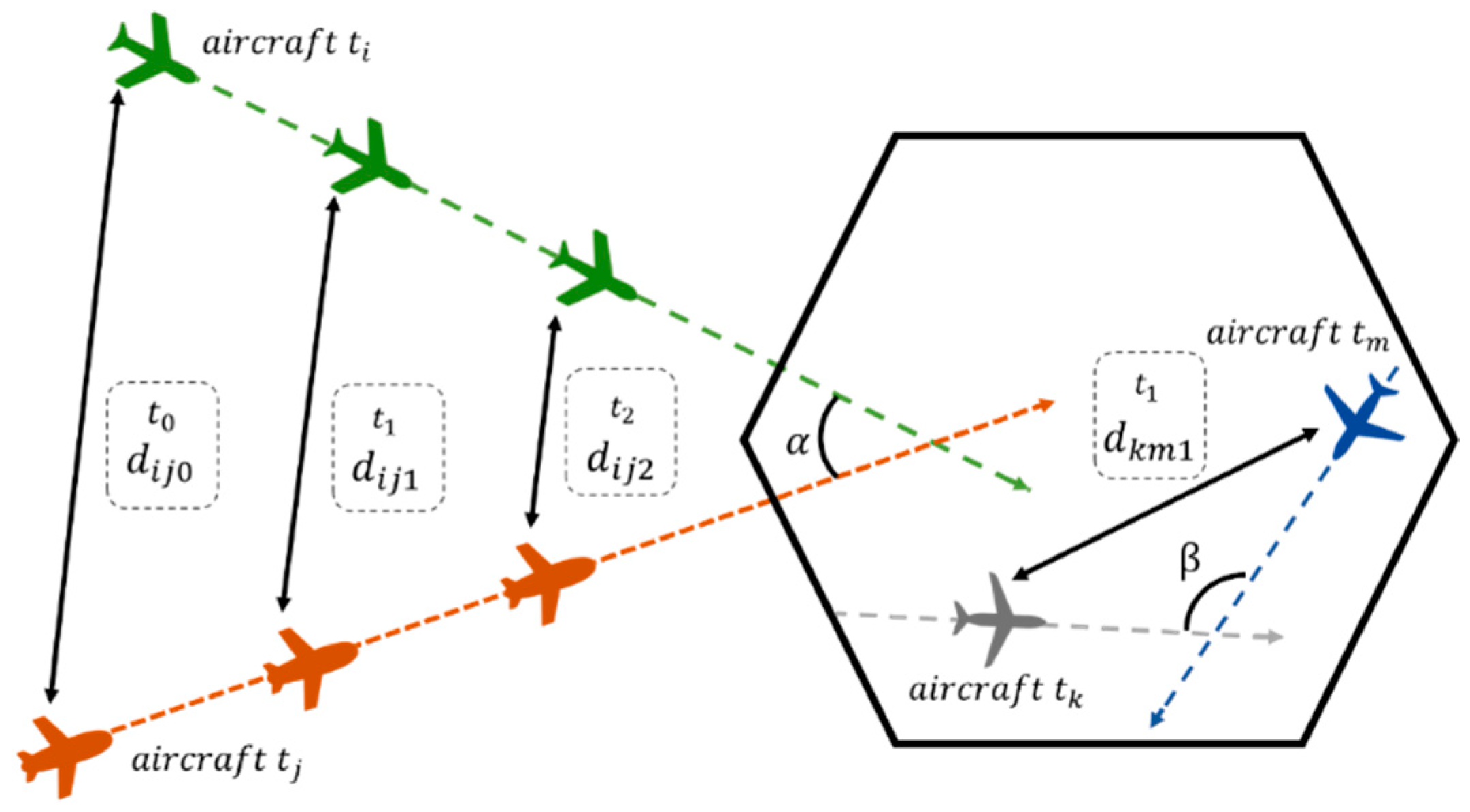
Based on real-time information on the aircraft speed, aircraft weight, FL, wind conditions (this information is provided by the aircraft) and the flight plan (FPL), the SMT tool will predict the aircraft trajectory of aircraft that are close to entering the sector in a short time, and the trajectory of the aircraft that are already in the sector. Furthermore, it will calculate the distance between predicted aircraft trajectories (Figure 1). The trajectory prediction module is considered to be included in the SMT. However, a current trajectory predictor external to the SMT could be used, and the predicted trajectories could be an input to the SMT. The prediction shall comply with a minimum quality factor to achieve the required level of accuracy.
A situation of interest (SI) is defined as a predicted situation in which the distance between an aircraft pair is going to be less than 10 NM [32]. If the SMT detects that an SI is going to occur, it shall start a searching process (in a huge database that holds all the Ad Hoc separation minima values) to determine the Ad Hoc separation minima applicable between this specific aircraft pair.
Therefore, the concept of SI is used for two reasons. The first is as a filter for the search of the Ad Hoc separation minima between a pair of aircraft in a huge database. Aircraft crossing at more than 10 NM are discarded from the Ad Hoc separation minima search process; if two aircraft cross at more than 10 NM, there is enough margin for the Ad Hoc separation minima not to be violated (the Ad Hoc separation minima are always equal to or less than the current horizontal separation value of 5 NM). Whereas, if two aircraft cross each other with a distance of less than 10 NM, the Ad Hoc separation minima values to be applied between a particular pair of aircraft are crucial. The second reason is that those SI are conflict situations, i.e., situations wherein the separation minima could be compromised in a short time horizon, and LOS (Loss of Separation) could occur. A SI is an input into the SMT conflict detection module of the SMT, which is referred to below.
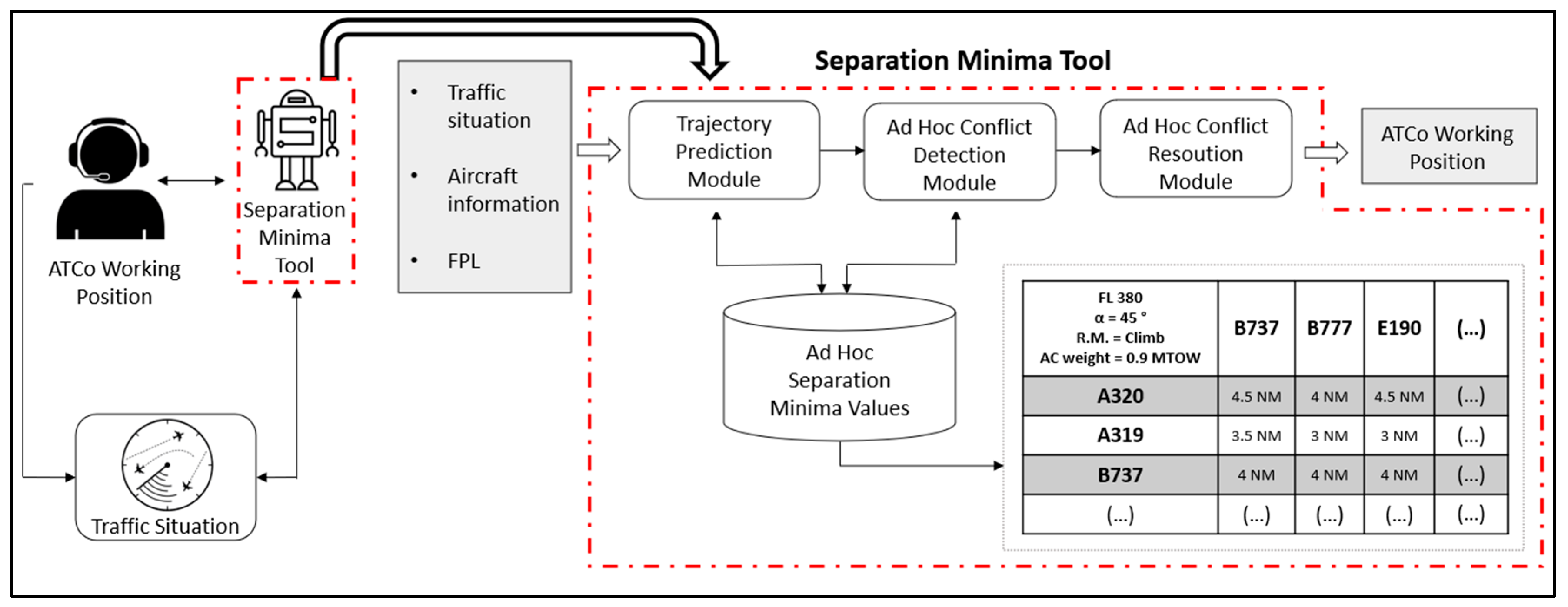
The first loop in the search process is to determine if both aircraft are flying in the same FL or not. If both aircraft are not flying in the same FL, the default value of separation minima is 5 NM and 1000 ft (i.e., the current values of separation minima). If both aircraft are flying in the same FL, the SMT searches in a huge database containing the Ad Hoc separation minima values for different situations and for this en route sector (Figure 2). The search process is as follows:
- Characterization of the SI: the SMT will characterize the SI according to the aircraft models, the aircraft weights, the speeds of the aircraft, the FL, the crossing angles between the trajectories, and the wind conditions.
- Once the SI has been characterized, the SMT shall search in the huge database for the Ad Hoc separation minima values according to the previous characterization. These separation minima values are predetermined and are associated with an AM in the vertical plane, i.e., climb or descent. An AM in the horizontal plane is discarded because it requires more time to avoid the collision. Therefore, the SMT would find the separation minima (for climb and descent) corresponding to the most similar situation to this real one in the sector (with a conservative judgement from a safety viewpoint).
- In this step, the SMT decides whether to apply the separation minima corresponding to the climb AM or to the descent AM. Therefore, the SMT shall check, in the vertical plane, whether there are aircraft in the FL immediately above or below the one at which the aircraft is flying.
There are three possible situations:
- If there are no nearby aircraft flying at the immediate upper or lower flight level, it shall choose the lower Ad Hoc separation minima, which will correspond to the descent AM.
- If there are any nearby aircraft flying at the immediate upper flight level, the aircraft disregards applying the Ad Hoc separation minima value corresponding to the “climb” AM, and chooses the separation value corresponding to the descent maneuver. The same applies to the opposite case, that of nearby aircraft flying at the immediate lower flight level.
- If there are nearby aircraft flying at the upper and lower flight levels, the default separation value of 5 NM shall apply.
The SMT is a dual-functional tool (Figure 2). On the one hand, it establishes the separation minima values for a given situation, based on the prediction module and the information it receives from the aircraft (wind vector, aircraft speed, aircraft weight, etc.). On the other hand, it has an Ad Hoc conflict detection and resolution module. That is, it detects, in the short term, if the distance between two aircraft is going to be less than the Ad Hoc separation value. In this case, it triggers an alert within a short time horizon (the default value is two minutes before the LOS, but it is a customizable value depending on the particularities of the scenario). After detecting that a LOS will occur, the SMT calculates the time instant at which the aircraft should be allowed to perform the resolution maneuver 10°, 20° and 30° vectors (track change) in the horizontal plane to avoid the LOS occurrence. That is, in order to avoid a LOS, a horizontal maneuver is allowed; however, as mentioned before, in order to avoid the collision, a vertical maneuver is performed.
3. Framework of the Ad Hoc Separation Minima Model
In this section, the framework within which the Ad Hoc separation minima are founded is presented. The model for the determination of the Ad Hoc separation is based on the approach of conceiving the separation minima as a barrier to collision. That is, they are a buffer to ensure that in case of a LOS, the situation does not develop into a collision. Therefore, the barrier to collision is the separation minima while the precursor to collision is the LOS.
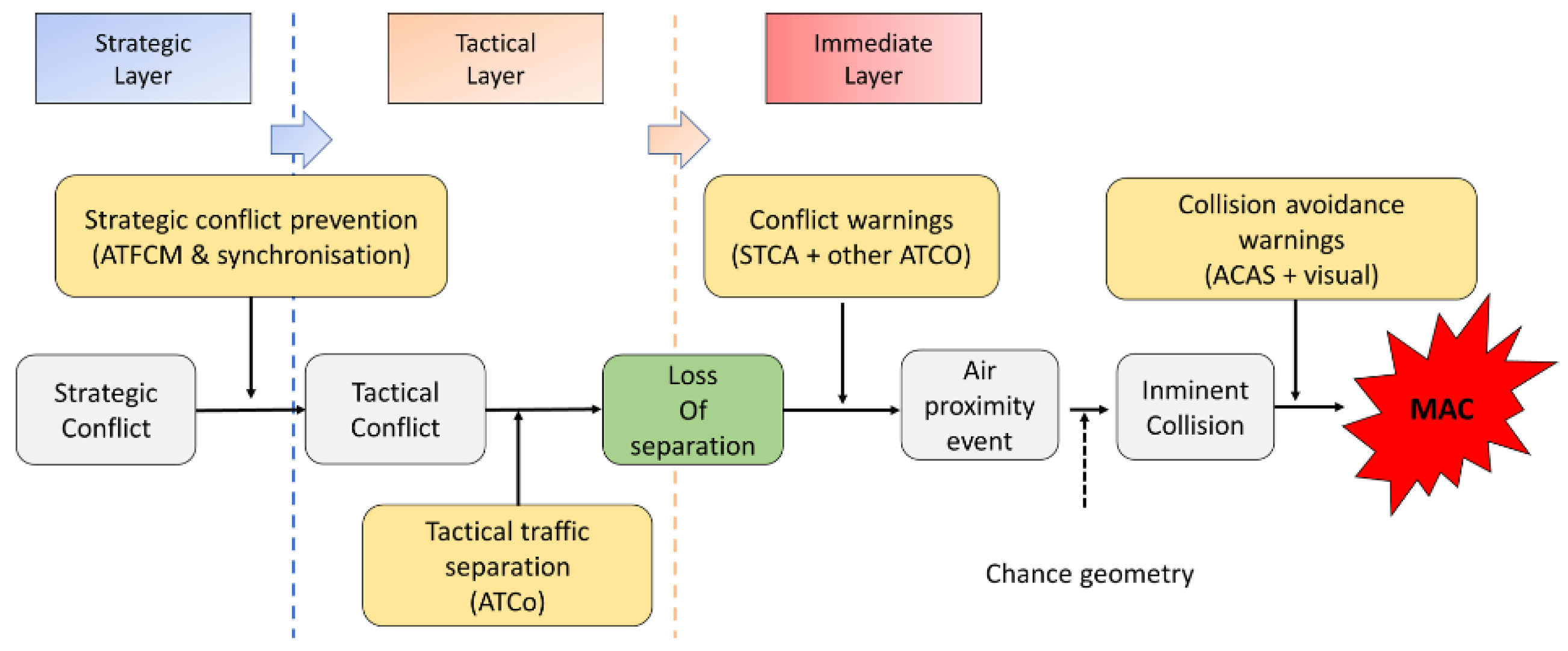
This notation of precursors and barriers is adopted from the Eurocontrol Integrated Risk Picture (IRP) model. This model states that the MAC (Mid-Air Collision) occurs as a consequence of a combination of barrier failures and the occurrence of precursors due to these failures. In Figure 3, this relationship is illustrated; it is the equivalent of a ‘Swiss cheese’ diagram (or Reason’s layered model). Barriers are indicated in yellow, while precursors are indicated in grey.
ICAO, in [31], defines the separation minima as the minimum displacements between an aircraft and a hazard (which could be another aircraft) that ensure the risk of collision remains at an acceptable level of safety. A key concept associated with the separation minima is the separation mode [31], which is an approved set of rules, procedures and conditions of application associated with separation minima. The reason that the Eurocontrol IRP model analyzes the precursor–barrier relationship from the strategic time horizon is because the values of the separation minima are associated with a form of operation (from the strategic layer, barriers are working in order to avoid the collision), and with a risk of collision that must be lower than a safe threshold.
In this research, the work is focused on the immediate layer in order to demonstrate if it would be operationally feasible to reduce the separation minima, and in which situations. Once it has been demonstrated that this would be feasible, the definition of the separation mode (strategic and tactical layers) for new separation minima values will be studied in future work.
For this reason, the Ad Hoc separation model is based on the IRP/Reason models and the Encounter Timeline concept (which refers to the set of actions that must be taken to avoid a LOS becoming a collision, in the temporal dimension). Therefore, it is a layer-based model in which the maneuverability of the aircraft and the human factor (HF) are considered. In particular, it is focused on the set of activities that must be performed in order to prevent a LOS from turning into a collision. According to [33], in which the contributing factors of a LOS are analyzed, the probability that a LOS occurs as a result of technical systems is practically negligible compared to the probability that a LOS occurs as a result of HF. Two fundamental variables of this model, which will be described in depth in the following section, are the Necessary Time and the Available Time.
The required time (which is called Necessary Time, ) is the time needed to perform the collision avoidance actions. The is made up of the time allocated to different actions: the time required by the ATCo to detect the LOS, the time to communicate the AM to the pilot, the reaction time of the pilot, the response time of the aircraft and the time required by the aircraft to complete the AM. The depends on the following factors: the aircraft model, the weight of the aircraft, the AM performed (climb or descent) and the FL at which the aircraft is flying. Therefore, it could be stated that it practically depends on the aircraft.
The Available Time to avoid the collision or the Time to the Closest Point of Approach (TCPA) is defined as the time since the separation minimum is lost until the closest point of approach (CPA). In the worst-case scenario, the CPA is the collision between aircraft. TCPA depends primarily on the geometry of the encounter, the aircraft velocities (closing speed rate) and the separation minima. Therefore, it may be stated that it depends on conditions outside of the aircraft itself (scenario, wind conditions, etc.).
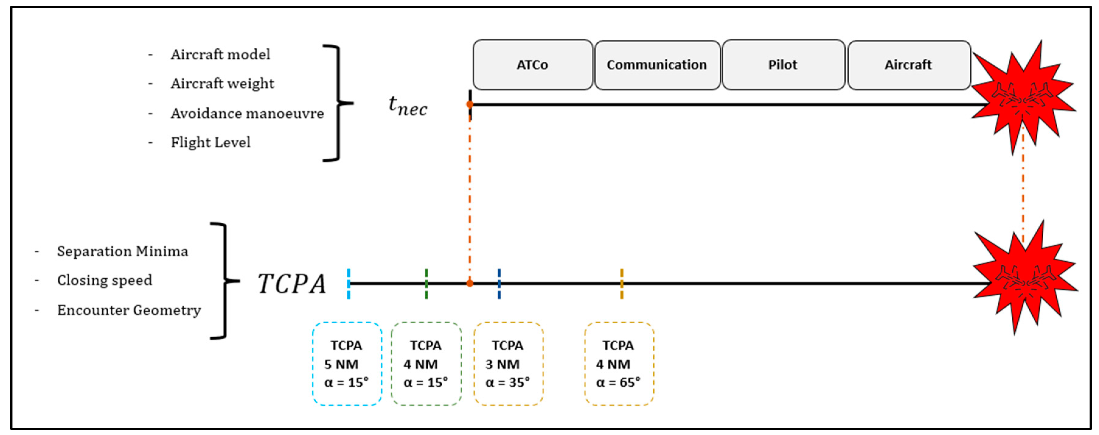
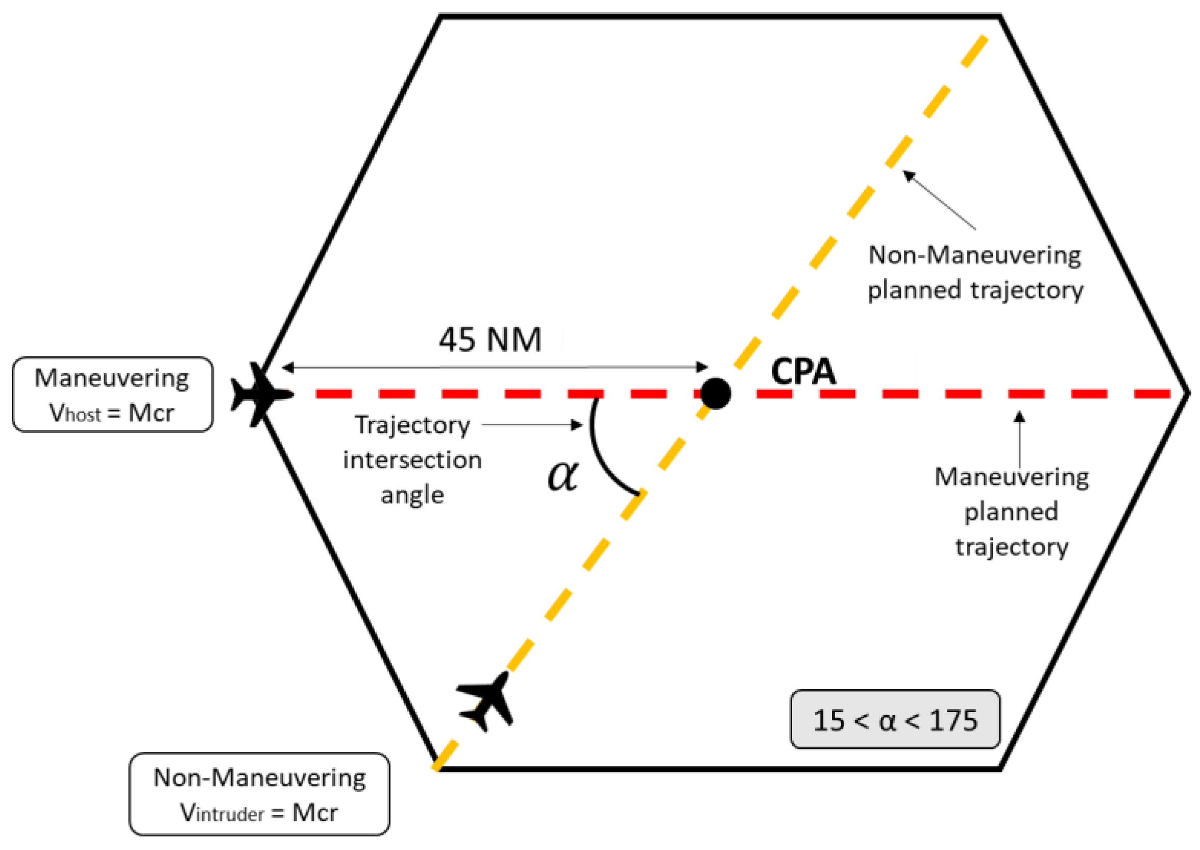
Thus, in relation to what has been mentioned, it can be stated that will be different for each aircraft and for different FL. That is, each aircraft has its own Maximum Take-off Weight (MTOW), and its own performance, which varies with FL. For example, climbing 500 feet to FL380 with an aircraft weight of 0.6 MTOW is not the same as climbing 500 feet to FL340 with 0.8 MTOW. The TCPA will be different for each encounter geometry, for the speeds of the aircraft and the applicable separation minima. It is noteworthy that equal TCPA values result from different situations (Figure 4). In other words, a TCPA of 40 s could be the result of an encounter geometry of 60° between tracks, aircraft speeds of 480 kt and separation minima of 5 NM, but it could also be the result of an encounter of 25°, aircraft speeds of 460 kt and 480 kt (aircraft 1 and aircraft 2’s speeds, respectively) and separation minima of 3 NM.
A collision is defined as a situation wherein the distance at the CPA (DCPA) between two aircraft, which have already lost the separation minima, is equal to or less than 500 ft (near MAC–NMAC distance, according to [34]), with the to perform the AM being greater than the TCPA (Equation (1)). As mentioned before, separation minima are understood as a barrier to collision. It is important to note that safety nets (such as TCAS) are not considered. This last requirement is in line with the ICAO [18] when examining separation minima.
The main assumption of this model is the following: those situations in which is lower than TCPA are potential situations in which the separation minima corresponding to this TCPA could be applied. This would imply that for the minimum separation applied to a particular situation for which the values of and TCPA have been calculated, the collision would not occur, as the AM could be executed. Therefore, the determination of the variables and TCPA is paramount. The calculation of these variables is explained in the next section.
4. Key Parameters of the Ad Hoc Separation Model
In this section, an overview of the method for the determination of the and TCPA variables is given. For this purpose, a scenario-based deterministic simulation model of geometric/intersection type was developed in MATLAB® (Figure 5). A worst-case scenario is designed, because the aim of these simulations is to provoke a collision and to obtain actual values of , for comparison with TCPA, which is also calculated in these simulations.
The specific inputs in the simulations are the initial position of the maneuvering aircraft in the horizontal plane and the initial velocities (or specific cruise Mach number for each aircraft model) of both the maneuvering and non-maneuvering aircraft. The simulation model is based on the following assumptions:
- Aircraft trajectories intersect at a specific angle;
- Simulations are calculated for different intersection angles (from 15° to 175° in 10° steps) in order to simulate a wide range of cases;
- The starting point of the non-maneuvering aircraft is calculated based on the angle between airways, given the initial position of the maneuvering aircraft, which is fixed. This is because the collision is being provoked (both aircraft reach the intersection point at the same time) in order to consider the worst-case scenario;
- Aircraft velocities are constant during the simulation of encounters;
- Aircraft fly at the same FL. This is because the model is applied to 2D. Simulations are performed separately for FL350, 360, 370, 380, 390, and 400;
- The model is deterministic. With these simulations, the collision is searched for the worst-case scenario. Therefore, uncertainties are not considered to facilitate the collision calculation;
- Four different aircraft models (AC1, AC2, AC3, AC4) are considered to simplify the study.
It should be noted that for confidentiality reasons, it is not possible to mention the specific aircraft models that have been used for the determination of the and TCPA. Three of them are medium-type (wake turbulent classification), and one heavy. This criterion is followed because the Ad Hoc separation concept will be applied to an en route upper airspace, and the aircraft mix in these airspaces is generally 90% medium and 10% heavy.
Throughout this section, we explain in detail how to obtain the and TCPA. These times are calculated using simulations based on the scenario and the assumptions defined above.
4.1. Necessary Time or Time Required (
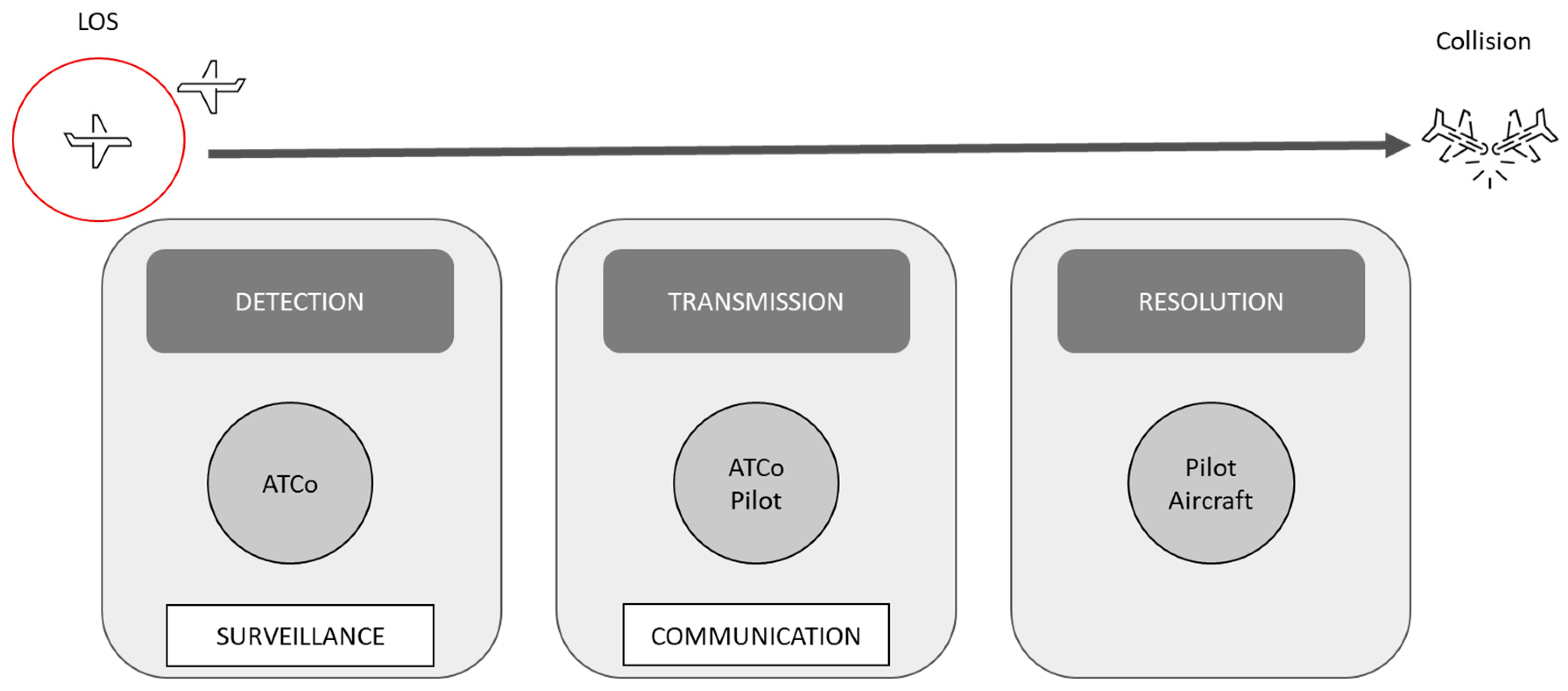
As mentioned before, is defined as the time required to perform a set of actions in order to prevent that a LOS becomes a collision. The is made up of the time allocated to three different actions: detection, transmission and resolution (Figure 6). This is in line with the Encounter Timeline concept [35,36,37]. An in-depth analysis of the parameters that constitute each layer is explained in the following sections. Once all the elements of each layer are defined, the is determined.
4.1.1. Detection Layer
The first component of the Encounter Timeline refers to the state information acquisition cycle and the evaluation step. This is the time required for the LOS detection by the ATCo ().
It is considered that the ATCo controls an en route sector. The ATCo receives information from surveillance sources (ADS-B and radar) each second. In addition, they perform their tasks proficiently. Therefore, the majority of losses of separation (LOSs) would be detected before they occur. Furthermore, the ATCo is assisted by the Short-Term Conflict Alert (STCA) system, or other functionalities that help him in the task of detecting conflict situations before they occur. The model is based on the worst-case scenario, which is that the ATCo realizes about the LOS when the separation minima between aircraft have already been lost. According to surveys conducted on ATCo, as well as the state of the art [38], the ATCo reaction time is modeled with a normal distribution, N(6.9;4.9) seconds (s), with 6.9 s of mean, and 4.9 s of standard deviation.
The ATC clearance of the AM that the ATCo has to communicate to the pilot is provided by the SMT, depending on the Ad Hoc separation minima determined for this specific encounter.
4.1.2. Transmission Layer
The transmission layer refers to the time required by the ATCo to communicate the ATC clearance for the resolution maneuver to the crew (). According to [39] the time required for the communication of ATC clearances in a critical situation in the en route phase can be modeled, using a normal distribution N(10.8;5.9) seconds, a mean value of 10.8 s, and a standard deviation of 5.9 s. This time is the addition of the time allocated to the following actions:
- Duration of the first ATCo transmission;
- Delay between the end of the ATCo’s initial transmission and the beginning of the pilot’s response;
- Duration of the pilot’s initial response to the ATCo’s first transmission;
- Duration of the ATCo’s second transmission to the same pilot;
- Duration of the second pilot response.
The fourth and fifth actions are included to consider the possibility that the pilot misunderstands the ATC clearance, which is detected by the ATCo in the pilot read-back procedure.
4.1.3. Resolution Layer
In the resolution layer, the pilot performs the collision AM. Therefore, it is necessary to consider the pilot reaction time to the ATC clearance (), the aircraft response time (), and the time required by the aircraft to execute the maneuver (). According to surveys conducted on commercial pilots, and the state of the art [40], the pilot reaction time could be modeled with a normal distribution N(5.7;2.3) seconds, with a mean value of 5.7 s and a standard deviation of 2.3 s.
The is calculated based on the Base of Aircraft DAta (BADA) 3 model [41]. BADA is an accurate aircraft performance model developed by Eurocontrol, which provides theoretical specifications to simulate the behavior of any aircraft. It is based on the ‘Total Energy Model (TEM)’, a three-degrees-of-freedom (3 DOF) model that relates the rate of work done by forces acting on the aircraft (Thrust and Drag) to the rate of the increase in potential and kinetic energy (Equation (2)). This initial 3DOF model becomes a 2DOF model when the lateral motion is ignored (i.e., the bank angle is equal to zero).
where
- —thrust acting parallel to the speed vector [Newtons]
- —aerodynamic drag [Newtons]
- —true velocity [m/s]
- —aircraft mass [kilograms]
- h—geodetic altitude [m]
- —gravitational acceleration [9.80665 m/s2]
- —time derivative [s−1]
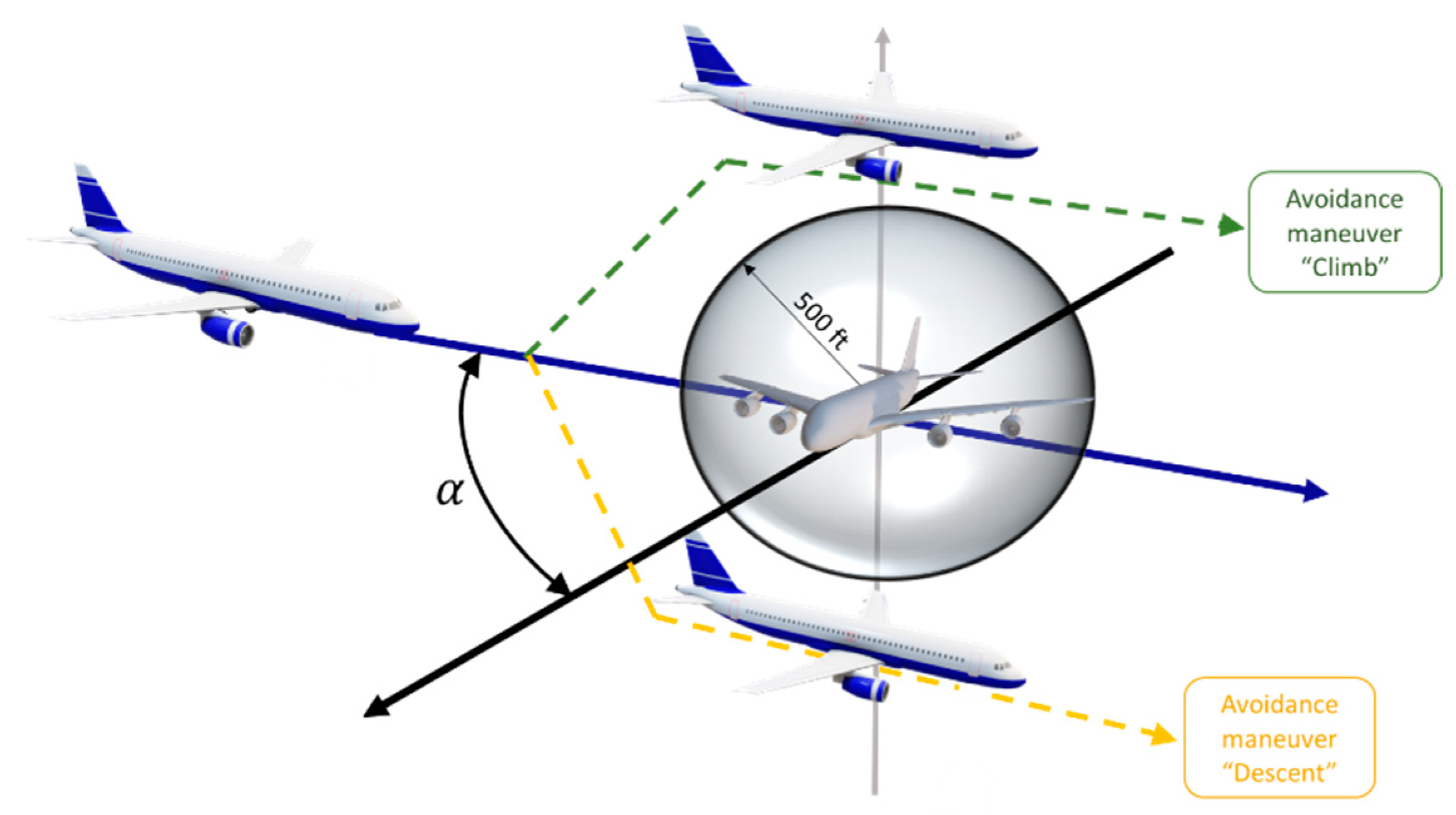
As detailed above, the worst-case scenario is considered during BADA simulations. This means that both aircraft (non-maneuvering and maneuvering) arrive at the intersection point of their trajectories in the same instant of time. It is considered that only one aircraft (maneuvering) performs the AM, which is always performed in the vertical plane (Figure 7). The AM ends when the distance between aircraft is equal to or greater than 500 ft, which is the NMAC distance [34]. Therefore, the time considered as the by the aircraft for the AM is the one needed by the maneuvering aircraft to climb or descent from the altitude at which both aircraft are flying, until a margin of 500 ft above or below the non-maneuvering aircraft is reached.
This has been calculated for each aircraft model with different FL and different weights in the simulations (as explained at the beginning of this section). Regarding the weight, five different weights, calculated as a percentage of the MTOW, are considered. The most conservative situation is for 0.9 MTOW weight, which means that the AM needs to be performed when the maneuvering aircraft has almost begun the cruising stage. In summary, the following assumptions are considered in the simulation (Table 1).
Climb AM
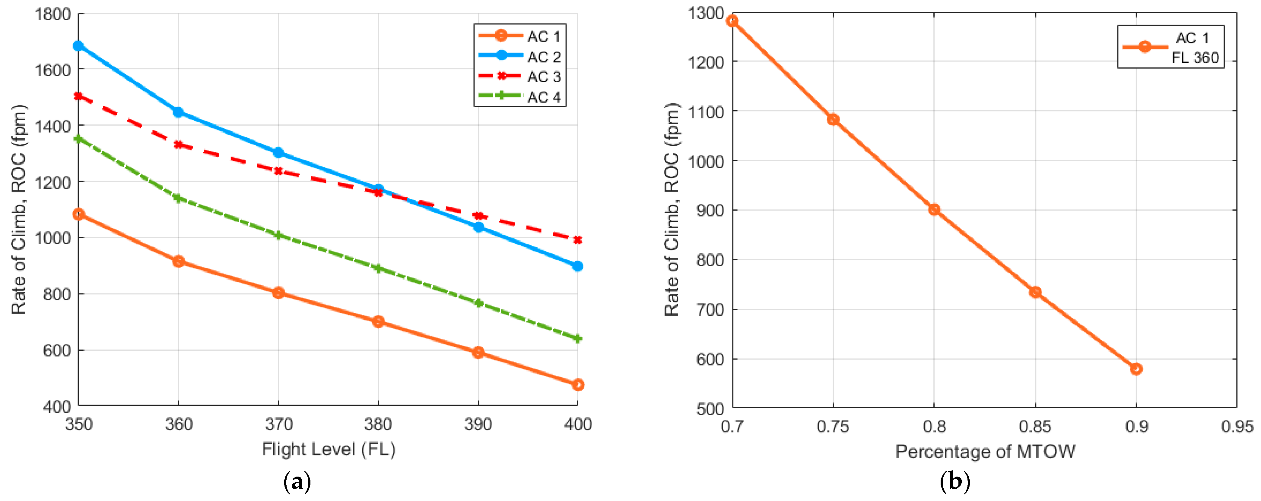
For the determination of the to execute the climb AM, the thrust and speed are set, and the Rate of Climb (ROC) is calculated. Therefore, the TEM equation is integrated in the following form (Equation (3)). The thrust considered in the simulation of the climb maneuver is the maximum. Regarding the speed, it is considered that in the en route phase, aircraft fly with their Mach cruise (provided by BADA), which is transformed into True Airspeed (TAS) from the speed of sound, using the ISA atmospheric model.
Table 2 shows the parameters used to simulate the climb AM for different aircraft models, and the mean value of the ROC calculated in the simulations. It is observed that AC2 is the one with the best performance.
In Figure 8a, the ROC variation with FL for the four simulated aircraft is shown. The ROC decreases as the altitude increases. In Figure 8b, for a specific aircraft and FL, the change in ROC with MTOW is simulated. The effect is the same as with the altitude; the ROC decreases when the weight increases.
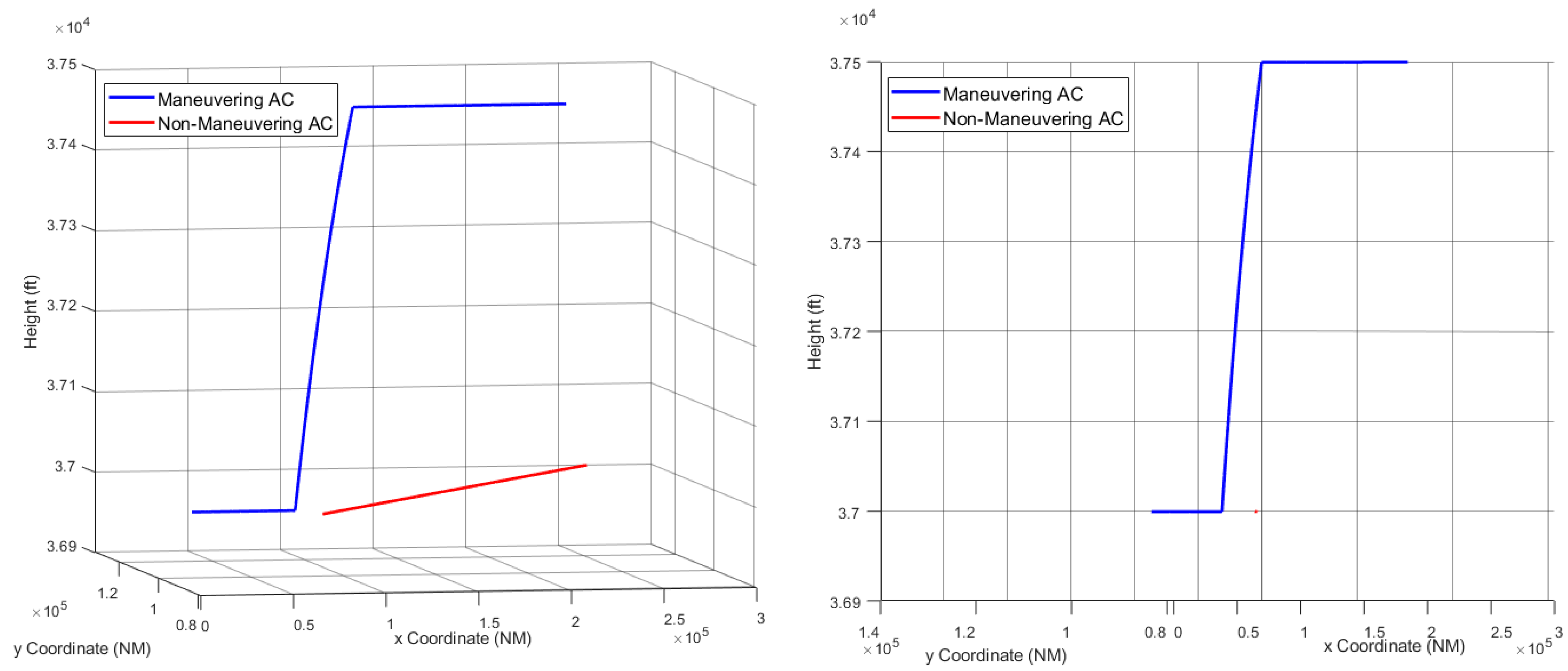
Figure 9 shows the climb AM performed by the maneuvering aircraft (blue line), while the non-maneuvering aircraft flies at a constant altitude (red line). These simulations have been performed for different aircraft pair models (that is, AC1–AC2, AC1–AC3, AC2–AC4), FL, and aircraft weights in MATLAB®. Here, only one pair is shown (AC1–AC2).
Descent AM
For the determination of the Rate of Descent (ROD), the procedure is similar to that followed for the climb AM. Nevertheless, the descent thrust is calculated as a ratio of the maximum thrust with different correction factors used for high and low altitudes. The results obtained from BADA for this maneuver showed an ROD in the order of 2000 to 2900 ft/min (Table 3).
ROD values of 2000–2900 ft/min are considered high. For this reason, the for the descent maneuver is calculated in two ways. The first one is based on the BADA results, assuming the ROD values obtained in the simulations. Using the second way, the value of is set at 1500 ft/min, based on the TCAS RA alert [42], which uses this value in a first filtering. Thus, when the ROD considered is 1500 ft/min, the to perform the AM is 20 s, and all aircraft perform it in the same way. For the descent maneuver, it is observed that AC2 is the one with the best performance, followed by AC1.
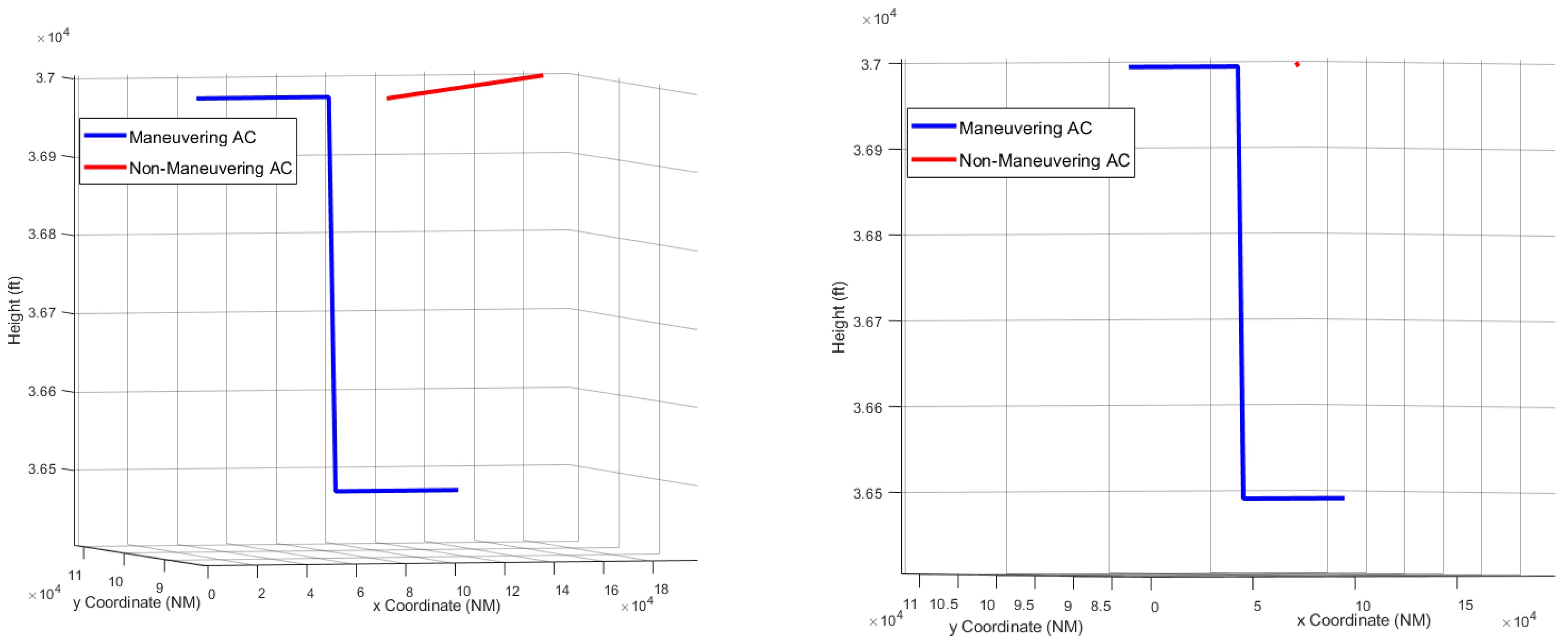
Figure 10 shows the descent AM performed by the maneuvering aircraft (blue line), while the non-maneuvering aircraft flies with constant altitude (red line). These simulations have been performed for different aircraft pair models (that is, AC1–AC2, AC1–AC3, AC2–AC4), FL, and aircraft weights in MATLAB®. Here, just one pair is shown (AC1–AC2).
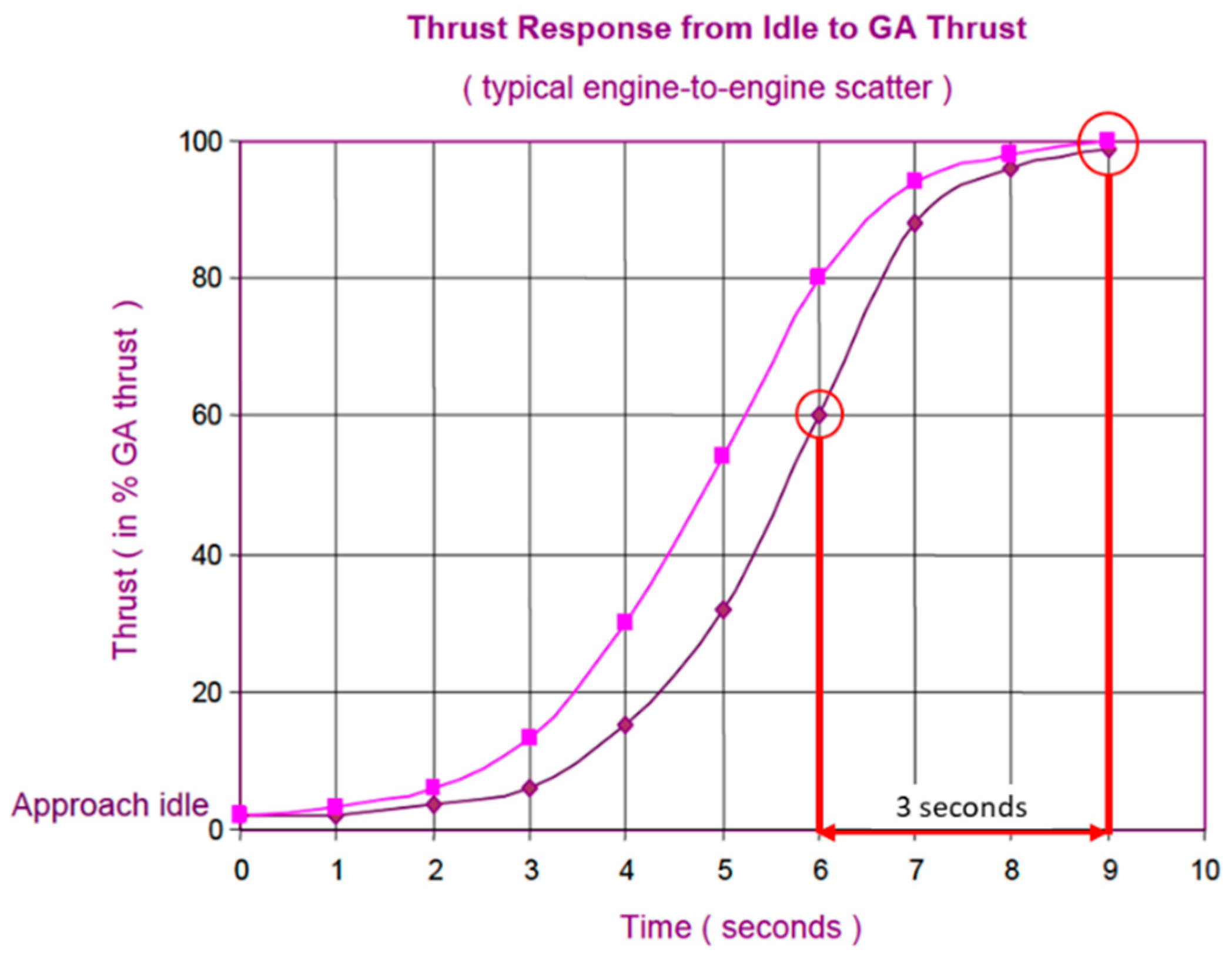
Regarding the response time of the aircraft (), it is defined as the temporal delay from the time the pilot triggers the maneuver until the aircraft begins to perform it. The time needed by the aircraft for a change from 60–70% thrust (cruise thrust) to maximum thrust (climb AM) is not zero; there is a response time on the part of the aircraft which is relevant for the determination of the parameter.
Thus, an analogy is made using data published by Airbus [43]. In particular, data are taken for aircraft that in the final approach segment (idle thrust) must perform a Go Around (GA) maneuver, in which the thrust is 100%. According to FAR–Part 33 certification, it must be ensured that no more than 5 s are taken to accelerate from 15% thrust to 95% thrust. Moreover, FAR–Part 25 and CS 25 [44] set a maximum of 8 s from idle to GA power. Assuming that in the en route phase, the aircraft is flying with 60–70% thrust, according to Figure 11, the aircraft needs 3 s to reach 100% of thrust (AM) from 60% of thrust.
4.1.4. Determination of
Once all factors have been explained in depth, the Necessary time () is determined using Equation (4):
It should be noted that the time related to HF () in Equation (4) is probabilistic, due to the fact that not all humans perform in the same way. Thus, and are modeled with a normal distribution. The normal distribution verifies the addition theorem. That is, given a set of independent normal random variables of different means and different variances, the sum variable of all will be distributed according to a normal distribution with the mean, the sum of the means, and with the variance, the sum of the variances [45]. Therefore, the sum of the and distributions is a normal distribution, called the HF distribution. As is known, for the standard normal distribution, 95% of the values are within 2 standard deviations of the mean (μ ± 2σ). For the HF distribution, this value is 40 s. Therefore, if 40 s is set, it could be said that 95% of situations are considered.
Moreover, it is noteworthy that since the time relative to HF is fixed (i.e., 40 s), what really makes the Ad Hoc for each aircraft model, FL, and weight is the variable, which is calculated with previous BADA simulations referred above.
4.2. Time to the Closest Point of Approach (TCPA) or Available Time
Another important variable in the model is the Available Time needed to avoid the collision or TCPA. This is defined as the time since the separation minima is lost until the CPA. In the worst-case scenario, CPA represents the collision between aircraft. TCPA depends primarily on the geometry of the encounter, the aircraft velocities, and the separation minima.
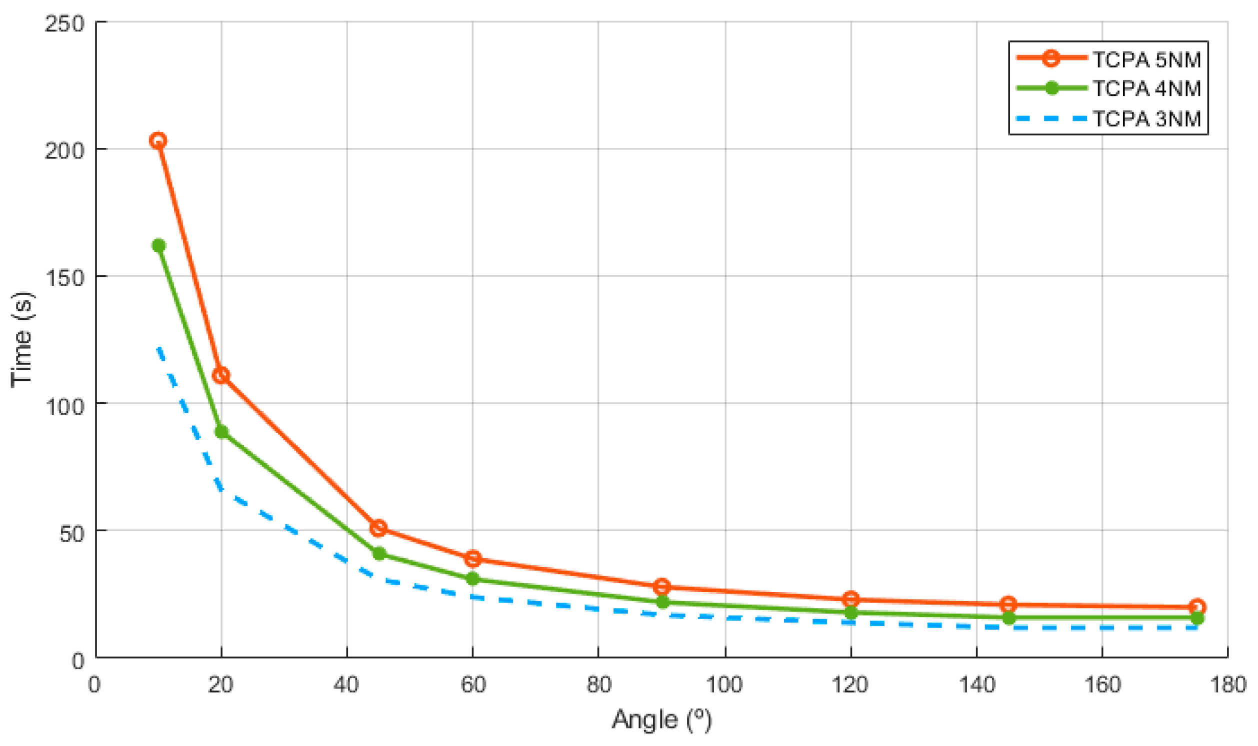
Figure 12 shows, for a specific encounter between an aircraft pair, how the encounter geometry (intersection angle) and the separation minima affect the TCPA. Depending on the angle of intersection, the geometry of the encounter can be overtaking (angles between 15–45°), crossing (45–135°), or head-to-head (H2H) encounters (135–180°) [46]. When the angle increases, the TCPA is lower, being the lowest with H2H encounters. With separation minima, the TCPA decreases if the separation minimum is reduced.
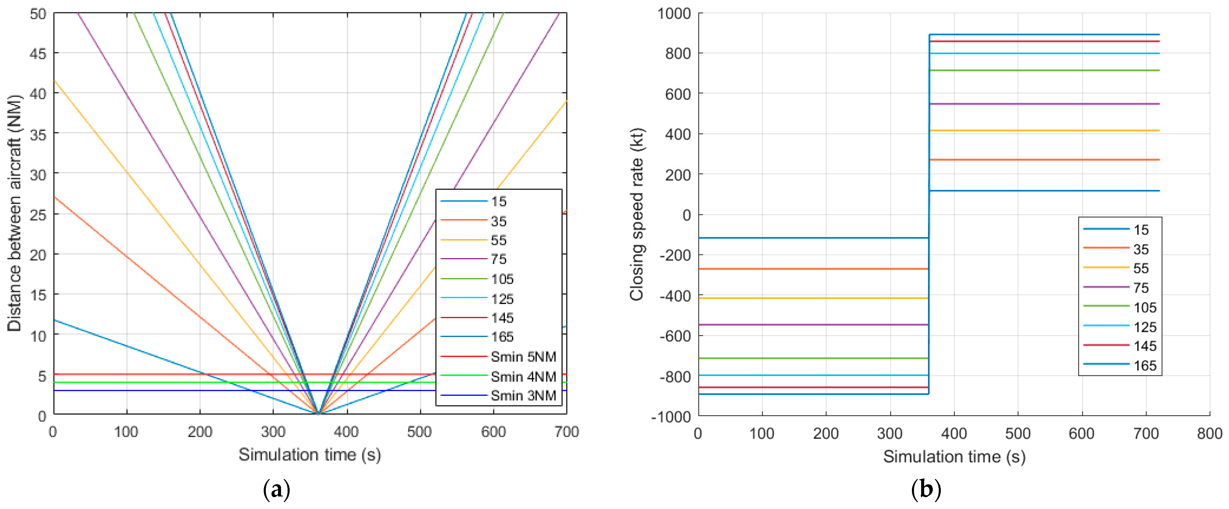
The influence of the speed of both aircraft on the TCPA is not as clear as the influence of encounter geometry and separation minima, due to the fact that the speed of aircraft, the entering points to the sector, and the distance from these points until the CPA are all important. This effect of distance to CPA and aircraft speed on TCPA can be understood, to some extent, through the closing speed rate, which expresses how fast aircraft are approaching as a function of aircraft speeds. The closing speed rate could be determined according to Equation (8) [47]. Parameters (Equation (7)) and stand, respectively, for the relative position and relative speed of the non-maneuvering (2) with respect to the maneuvering aircraft (1), while and (Equations (5) and (6)) are the relative position and speed at the initial time.
Figure 13 represents the evolution of the distance between aircraft pairs in the simulations performed (Figure 13a), and the closing speed rate (Figure 13b). The closing speed rate corresponds to the derivative of the distance evolution curve between the aircraft pair. The distance evolution curve is U-shaped for all encounters, except when there is a collision between the aircraft pair, which is V-shaped. Because collision is triggered in these simulations, the curves of Figure 13a are V-shaped. Only a few angles are depicted in Figure 13a, where in addition to the distance evolution plot, there are three horizontal lines corresponding to the separation minima values: 5 NM (red), 4 NM (green) and 3 NM (blue). For larger intersection angles, the curve closes, resulting in a lower TCPA. The lower the separation minima value, the lower the TCPA. In Figure 13b, the closing speed rate values are higher for larger intersection angles. Hence, the higher the intersection angles, the higher the closing speed rate and the lower the TCPA.
5. Results
In this section, the results obtained from the determination of and TCPA variables that have been calculated from previous simulations are shown. Given that the application of Ad Hoc separation is feasible whenever < TCPA, a comparison is also made between these two variables in order to obtain, a priori, those situations in which Ad Hoc separation could be applied. Obtaining the values of the Ad Hoc separation minima for each specific situation is beyond the scope of the study presented in this paper. Moreover, according to the definition of separation minima, these values should be subjected to a risk assessment, as established by the ICAO in [18].
5.1. tnec Results
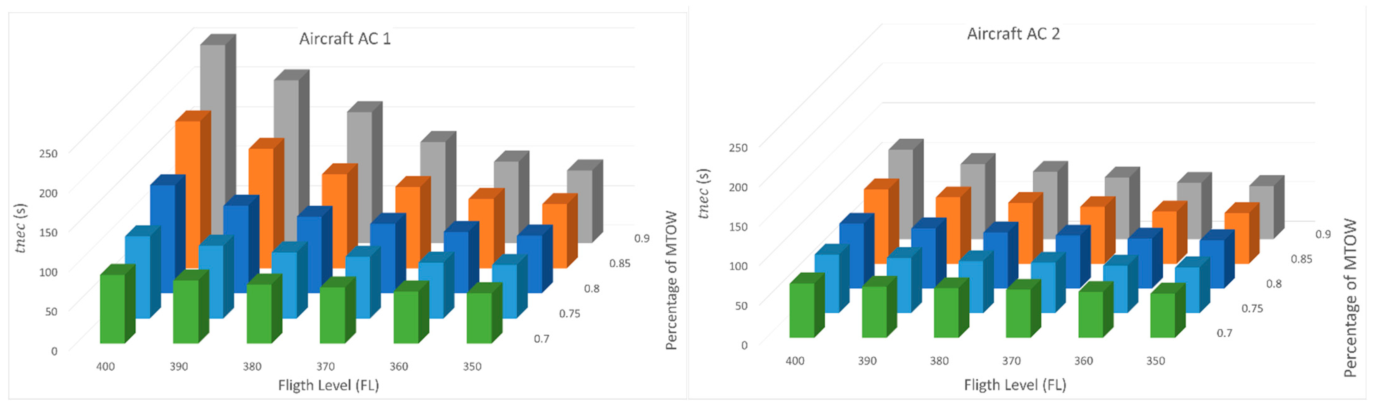
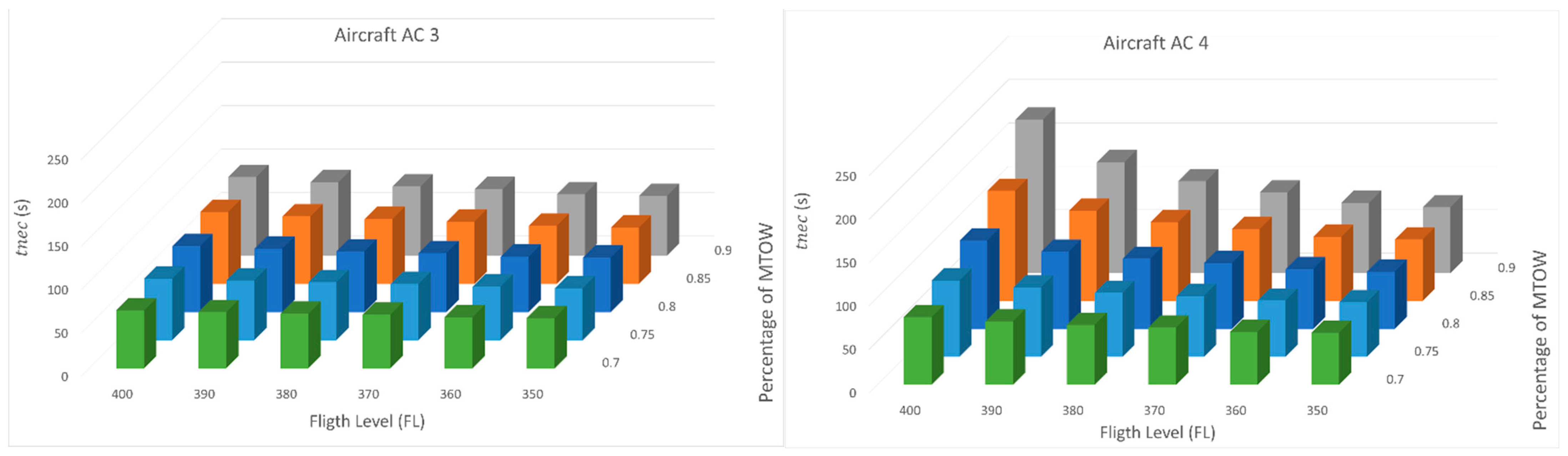
The following Figure 14 shows the variation in the with FL and weight for different aircraft models performing a climb AM. As expected, aircraft require more time to perform a climb maneuver at higher FL (always below their operational ceiling). The same is true for the weight. The greater the weight, the longer the .
Among the four aircraft models in the study, AC 1 (M) is the one with the highest values for the for a climb AM. It is noteworthy that AC 4 (H) requires less time than AC 1. In turn, AC 2(M) and AC 3(M) present similar values of Necessary Time, although AC 3 has better performance for higher FL.
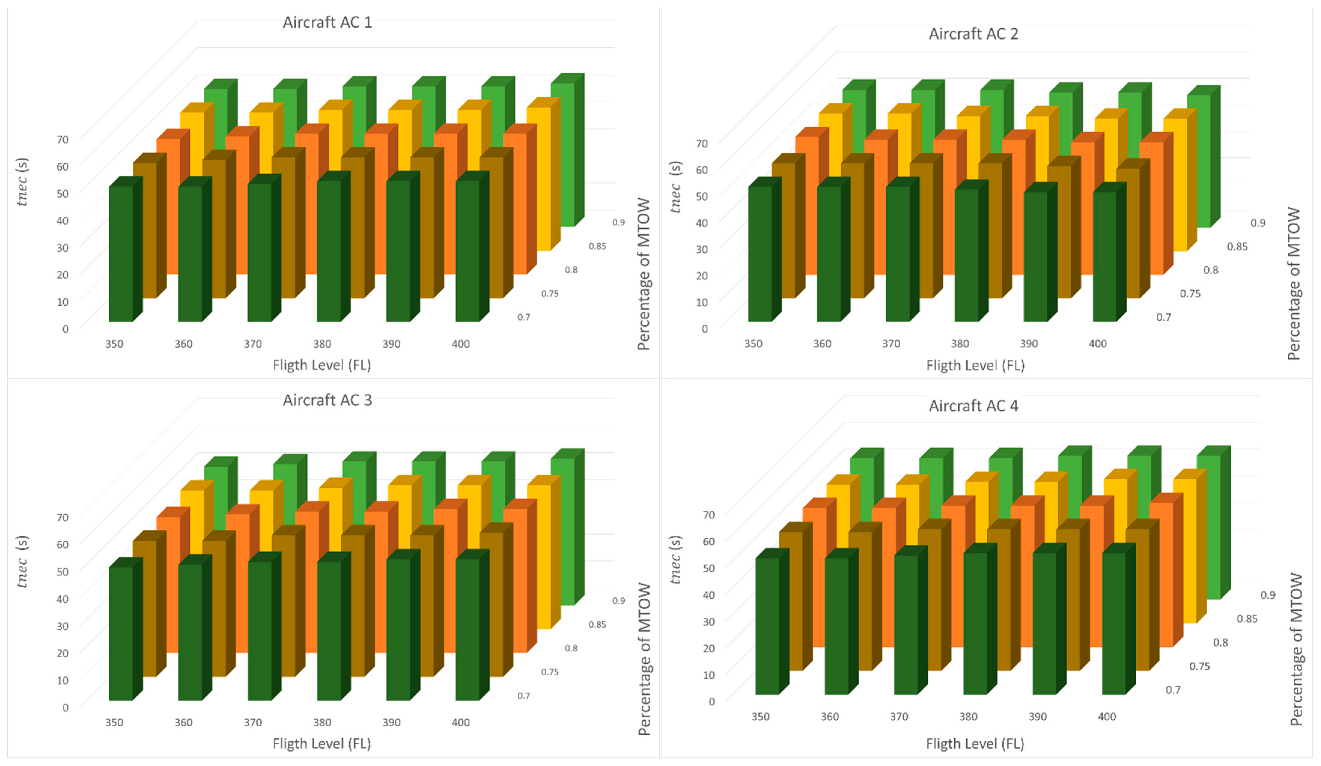
The for the descent maneuver is presented in Figure 15. It is observed that the values are practically of the same order of magnitude for all the aircraft models analyzed, being shorter than those required for the execution of the climb AM.
The variation in the for the descent AM with weight and FL is the same as for the climb AM. The higher the FL and the greater the weight, the more time the aircraft requires to execute the descent maneuver. However, this variation is practically negligible, as the difference is 2–3 s between FL 400 and FL 350 and 0.7 MTOW and 0.9 MTOW. The results presented are calculated considering that the ROD is not limited. If the ROD is limited to 1500 ft/min, the results are the same for all aircraft, all FL and all weights.
5.2. TCPA Results
Regarding the TCPA, Figure 16 and Figure 17 show its variation with different parameters. As mentioned above, the TCPA decreases when the separation minimum is reduced. Additionally, it decreases when the intersection angle is higher due to the fact that the closing speed rate increases when the intersection angle is greater. In Figure 17, TCPA values are calculated for aircraft encounters of MM, MH and HH aircraft pairs, as a function of different intersection angles. This is because the Mach cruise for M aircraft and H aircraft is not the same; hence, the TCPA depends on the specific encounter. Nevertheless, as can be shown, the temporal difference in seconds between the TCPA values for different encounters is negligible.
5.3. Results of the tnec vs. TCPA Analysis
Situations of interest are those in which the is lower than the TCPA. Therefore, both variables are now contrasted in order to detect those situations in which the reduced separation minima (corresponding to the calculated TCPA in each case) could be applicable. As a result, different separation minima could be defined depending on the different situations (Ad Hoc separation concept), thus demonstrating the feasibility of this concept.
Figure 18 shows, for a climb AM performed by the maneuvering aircraft, for different maneuvering aircraft weights and different FL and for a HF value of 40 s, what the maximum possible angle between tracks would have to be to ensure that the never exceeds the TCPA, calculated for a separation minimum of 5 NM. Different geometries have been considered (angles between tracks from 15° to 175°), in each case obtaining the highest possible value of the angle between tracks.
The best results are obtained for AC 3, while the worst are for AC 1. The maximum value between tracks for this specific case is 35°, in order to ensure that is lower than TCPA for each specific situation. It should be noted that when the ‘best results’ are mentioned, we refer not only to higher angle values but also to more situations in which this higher angle can ensure that is lower than TCPA. For instance, an angle of 35° between tracks is only possible in one situation (FL350 and 0.7 MTOW), for AC 1, while for AC 3, eleven different situations are possible.
The notation N/A appears in some cells, indicating that it would not be possible for that maneuvering aircraft to perform a climb AM for that given FL and the specified weight conditions. This may be either because the FL is close to its operational ceiling, or because the combination of that FL and those generally restrictive weight conditions means that the is far in excess of the TCPA for any of the possible angles. It should be noted that climb AM gives the worst result in comparison with the descent maneuver for the limited and the unconstrained ROD. Moreover, 40 s has been considered for the HF value; however, it is a rather restrictive value that has been obtained from the values of ATCo and pilot reaction time and communication time that were obtained some years ago.
When reading these results (Figure 18), it is important to consider the following. The angle value appearing in each cell indicates that collision avoidance is possible if the separation minima between that aircraft pair and for that specific situation (FL, weight and AM) correspond to that TCPA. This is true for the angle between tracks or for any angle smaller than indicated.
It is striking that for a current separation value of 5 NM, the intersection angles between aircraft tracks are limited. However, there are two issues to take into account. Firstly, a worst-case scenario is being considered in the simulations, in which the aircraft arrive at the point of intersection between airways at the same time (collision), which is a rather less probable situation. Secondly, and more importantly, it should be considered that this study strictly analyzes, in terms of encounter geometry, aircraft performance and speeds, whether with a given separation minima value it is possible to perform the AM in 100% of the cases ( < TCPA), that is, only the immediate layer from the IRP Model is being considered. However, according to the ICAO definition, the defined separation minima values are also associated with a separation mode (strategic and tactical layers in IRP Model) and a risk of collision. Therefore, other elements need to be considered for a complete picture of the system; however, these are outside the scope of this research, and will be considered in future work. For instance, nowadays, the number of situations in which there would not be time to execute an AM with a 5 NM separation is limited (e.g., opposite flights flying at different FL and not in the same FL); the ATCo most often resolves any conflict situation long before it occurs, and the TCAS system often triggers before the separation between two aircraft is lost.
It should be noted that no new separation minima values are being defined. To do this, as mentioned above, a risk assessment is required, which is beyond the scope of the research presented in this document, and will be performed in future work. However, these results show that it would be operationally feasible to apply different separation minima values for different situations (Ad Hoc ConOps).
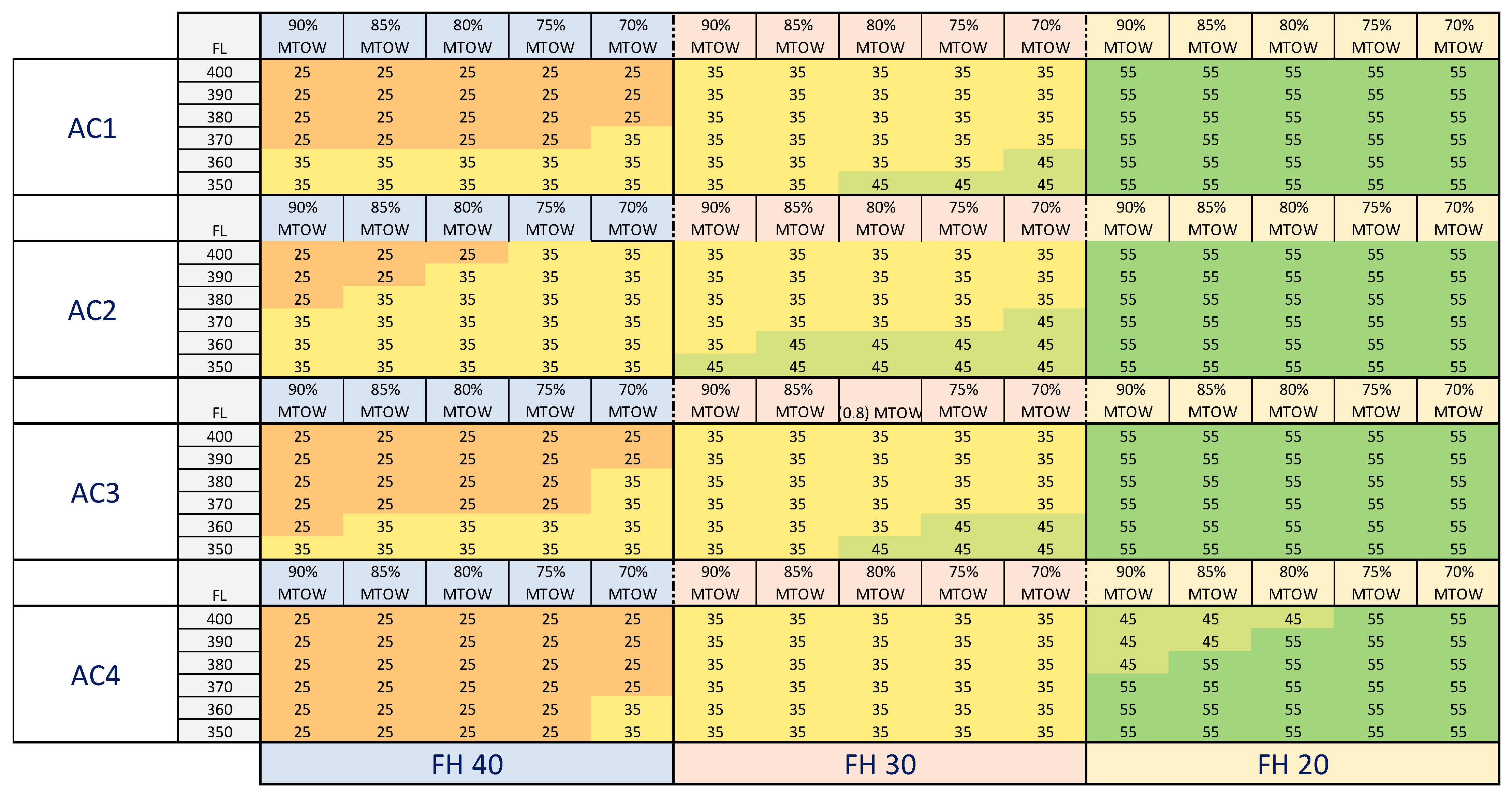
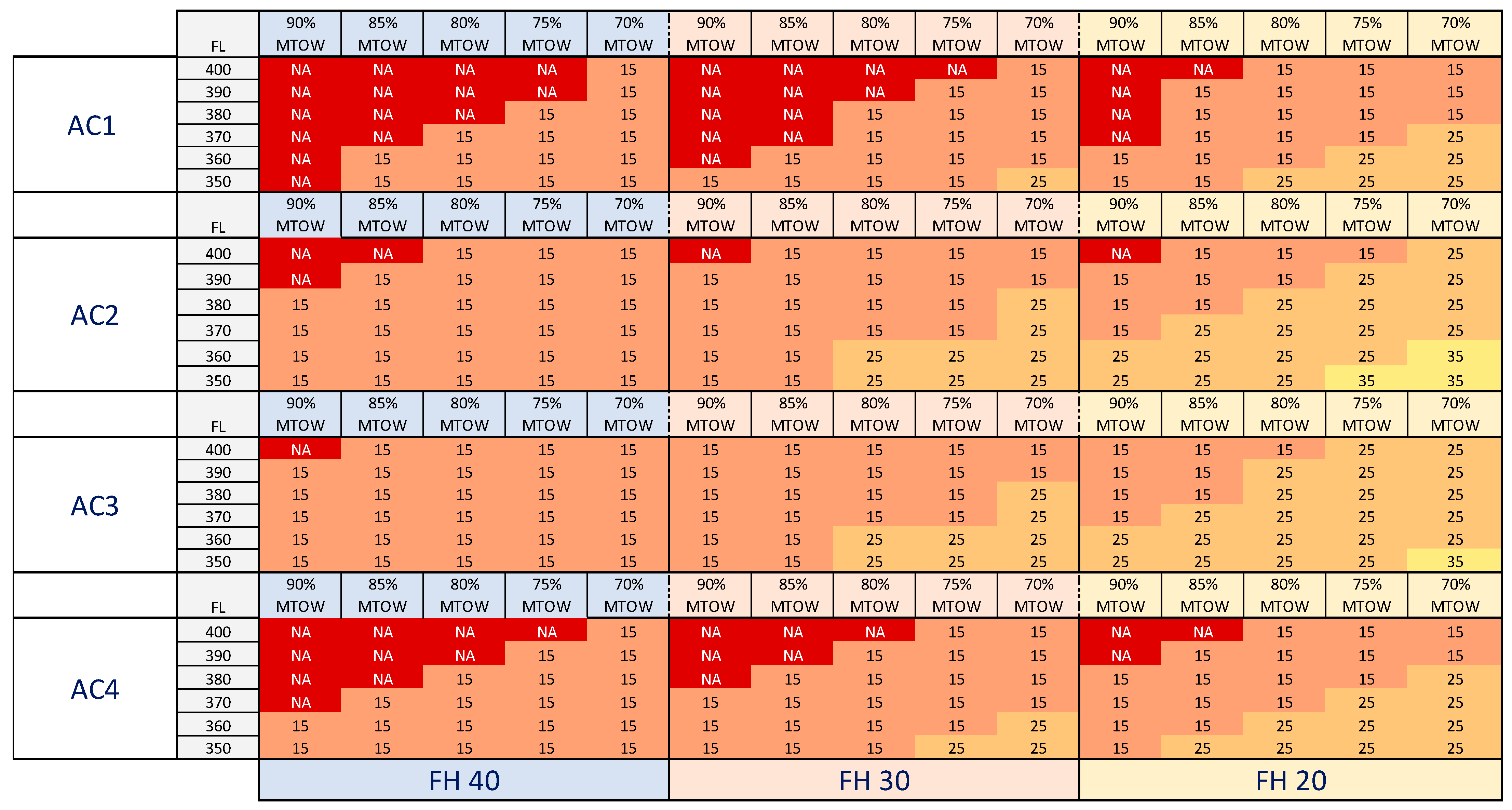
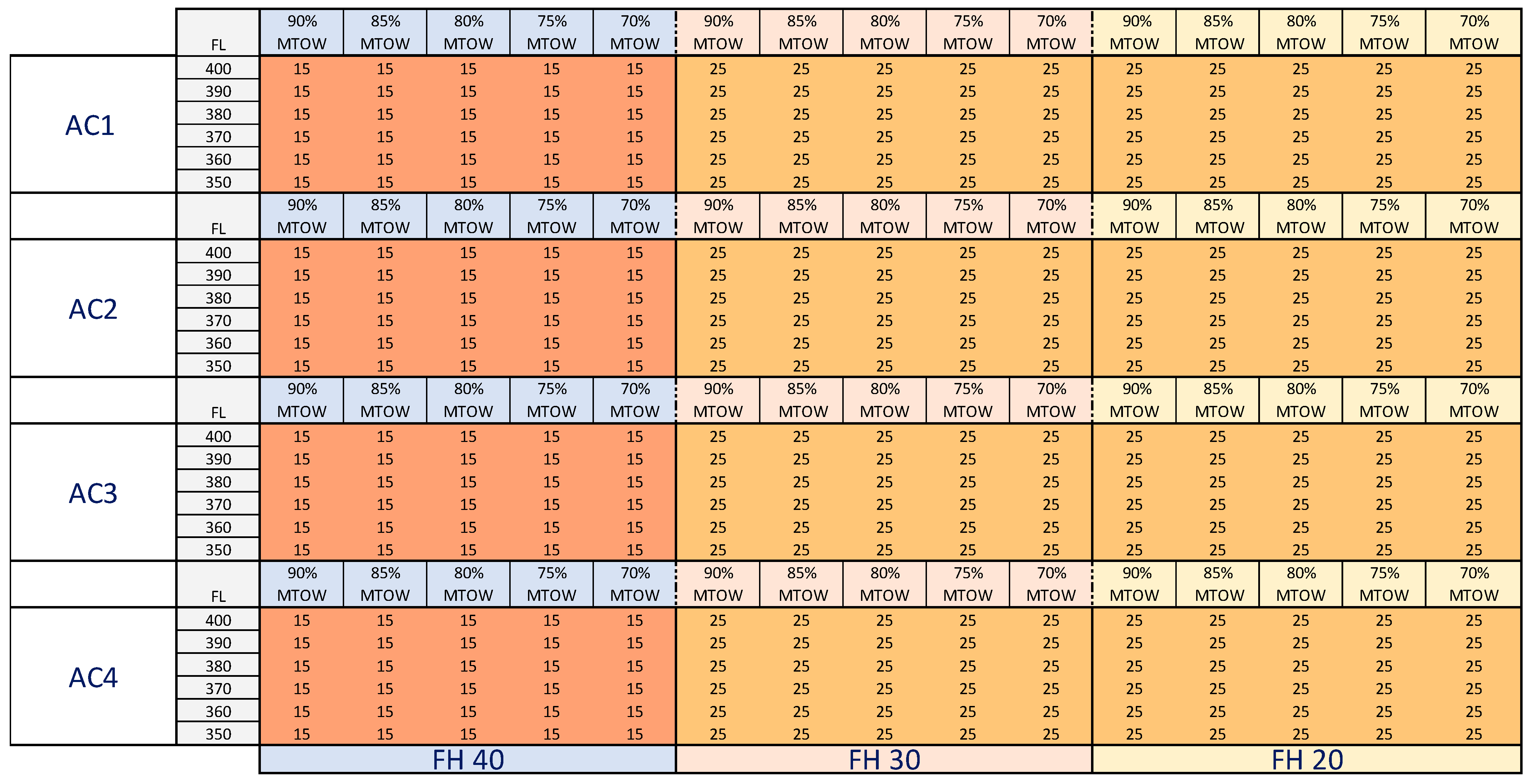
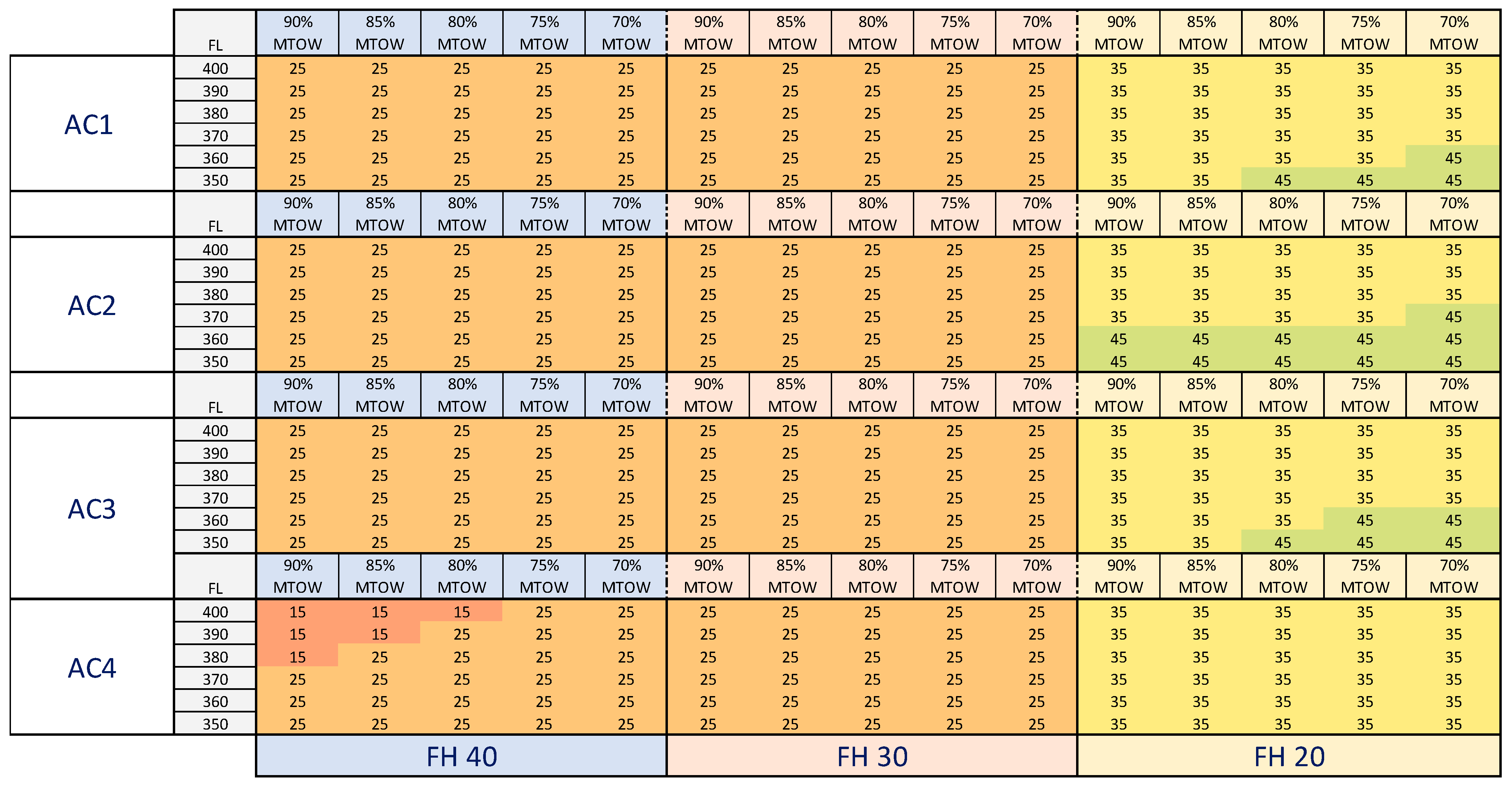
In Appendix A, the rest of the results calculated for limited descent and unconstrained descent and for separation minima values of 3 NM and 4 NM are presented. The results are displayed in a heat map to aid in understanding the best (green) and worst (red) results. Different HF times have been considered (40, 30, and 20 s), since when calculating the variable, the largest contribution is due to the HF, while the smallest is relative to the time required by the aircraft to respond and perform the AM. The time relative to the HF can be reduced from 40 to 30 or 20 s, depending on the ATC support tools. Through this factor, it is possible to envisage how an advance in technology could reduce the times relative to the HF, and how this would lead to a greater number of situations in which a lower separation minima than the actual one could be applied.
As expected, it is observed from the results of Appendix A that the most restrictive angle values occur for the TCPA corresponding to 3 NM and for the climb AM. The best results are obtained for descent maneuvers for an unconstrained ROD, considering that the preferable situation is one in which the angular difference between tracks is larger. Looking at the results, it is noteworthy that in any specific situation, higher intersection angles of 75° are possible, which means that the feasibility of implementing this concept is greater for geometries with smaller angles. Finally, since different HF values were considered in the simulations in order to analyze the sensitivity of this parameter within the results, it should be noted that a reduction of 10 s in the HF time means the possibility of increasing the angle between tracks by 10°, while ensuring that the is lower than TCPA.
6. Conclusions
One of the main challenges facing the ATM system is the need to increase airspace capacity, which is already close to saturation in many cases. Separation minima are one of the determining factors of airspace capacity. For this purpose, in this paper, a new concept is proposed, that of Ad Hoc separation minima. Ad Hoc or Variable separation minima refer to the application of different separation minima values between aircraft pairs in the same volume of airspace depending on a set of factors (aircraft models, FL, aircraft weight, encounter geometry, AM, HF). This concept addresses the current problems of lack of airspace capacity, and the fact of trying to benefit from better equipped and better performing aircraft as a consequence of the advancement of technology in recent decades.
The factors that define these Ad Hoc separation minima and their relationships are discussed in this research, and a model for their determination is presented. The operational feasibility of this new concept has been analyzed through simulations.
The results obtained in the simulations show that separation minima could be reduced in more situations in which the unconstrained descent AM is performed, and the aircraft type is AC3. The worst results are obtained for the climb AM and by the AC1 type.
The sensitivity of the model to the HF time shows that a reduction of 10 s in the HF time leads to the possibility of an increase of 10° in the angle between tracks. Looking at the results, it is noteworthy that in any specific situation, higher intersection angles of 75° are possible, which means that the feasibility of implementing this concept is greater for geometries with smaller angles.
The main contributions of this study answer the research questions raised in the introduction of this paper, and are summarized as follows:
- It has been demonstrated that it is possible to reduce the separation minima;
- It has been proven that reductions in the separation minima are not applicable in general, but in particular situations;
- The different situations in which the separation minima could be reduced (depending on the encounter geometry, aircraft models, aircraft weights, FL, AM and HF) have been identified.
In view of the above, it is inferred that this new concept is operationally feasible. Since each separation minimum has a separation mode associated with it, reducing the separation minima in certain situations involves defining or modifying the separation mode, which will be achieved in future work.
It should be noted that a full validation of the concept has not been performed, as an assessment of the technical enablers has not been included, but is reserved for future work; however, it has been shown, in a brief form, that an improvement in the given technology would lead to a reduction in the current separation minima. In particular, an improvement in the communication system and support tools for the ATCo and the pilot would reduce HF times from 40 to 20 s, leading to the possibility of an increase of 20° in the angle between tracks.
In addition to the above findings, four areas in which research could be improved have been identified: (1) the development of the Ad Hoc separation minima values based on risk assessment and the definition of the separation mode; (2) the definition of the CNS requirements for the safe implementation of this concept; (3) the development of a SMT tool based on Ad Hoc separation minima to assist the ATCo and reduce HF time; and (4) the validation of the concept in terms of the key performance areas of capacity and safety.
Author Contributions
Conceptualization, L.S.-M., L.P.S. and J.A.P.-C.; methodology, L.S.-M. and F.N.; software, L.S.-M. and I.G.M.; validation, L.P.S., J.A.P.-C. and F.N.; formal analysis, L.S.-M. and F.N.; investigation, L.S.-M. and J.A.P.-C.; resources, L.P.S. and E.S.A.; data curation, L.S.-M. and I.G.M.; writing—original draft preparation, L.S.-M.; writing—review and editing L.P.S., J.A.P.-C., F.N. and E.S.A. All authors have read and agreed to the published version of the manuscript.
Funding
This research received no external funding.
Acknowledgments
Notably: the authors would like to acknowledge Julio Olavarria Fernández, an ATCo from ENAIRE. Moreover, the authors acknowledge ISA Software, who granted us the license to use RAMS Plus. This tool has been crucial for validating our results.
Conflicts of Interest
The authors declare no conflict of interest.
Appendix A. Results of the Comparison between tnec and TCPA
- TCPA–5 NM
Figure A1 shows the results for the climb AM obtained for the TCPA calculated for a minimum separation value of 5 NM.
Figure A1.
Climb AM results. TCPA 5 NM.

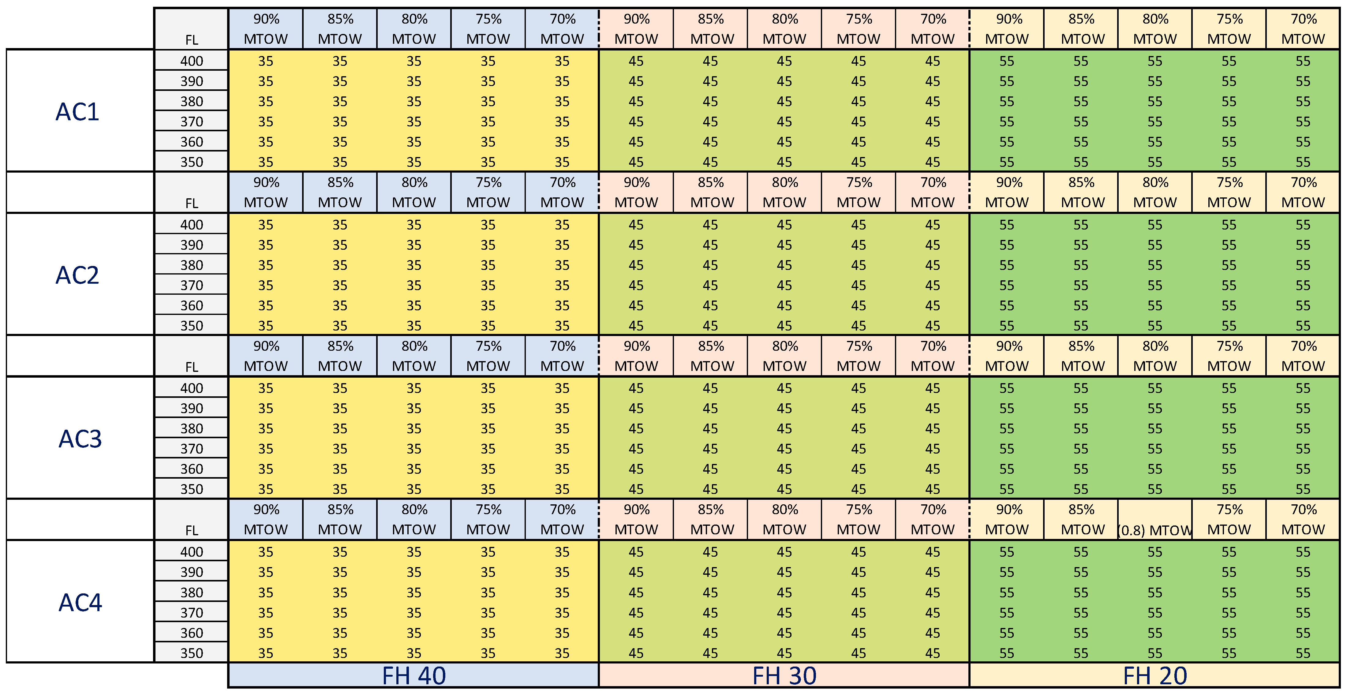
Figure A2 shows the results for the descent AM obtained with an ROD limited to 1500 ft/min for the TCPA calculated for a minimum separation value of 5 NM.
Figure A2.
Descent AM results, ROD limited to 1500 ft/min. TCPA 5 NM.

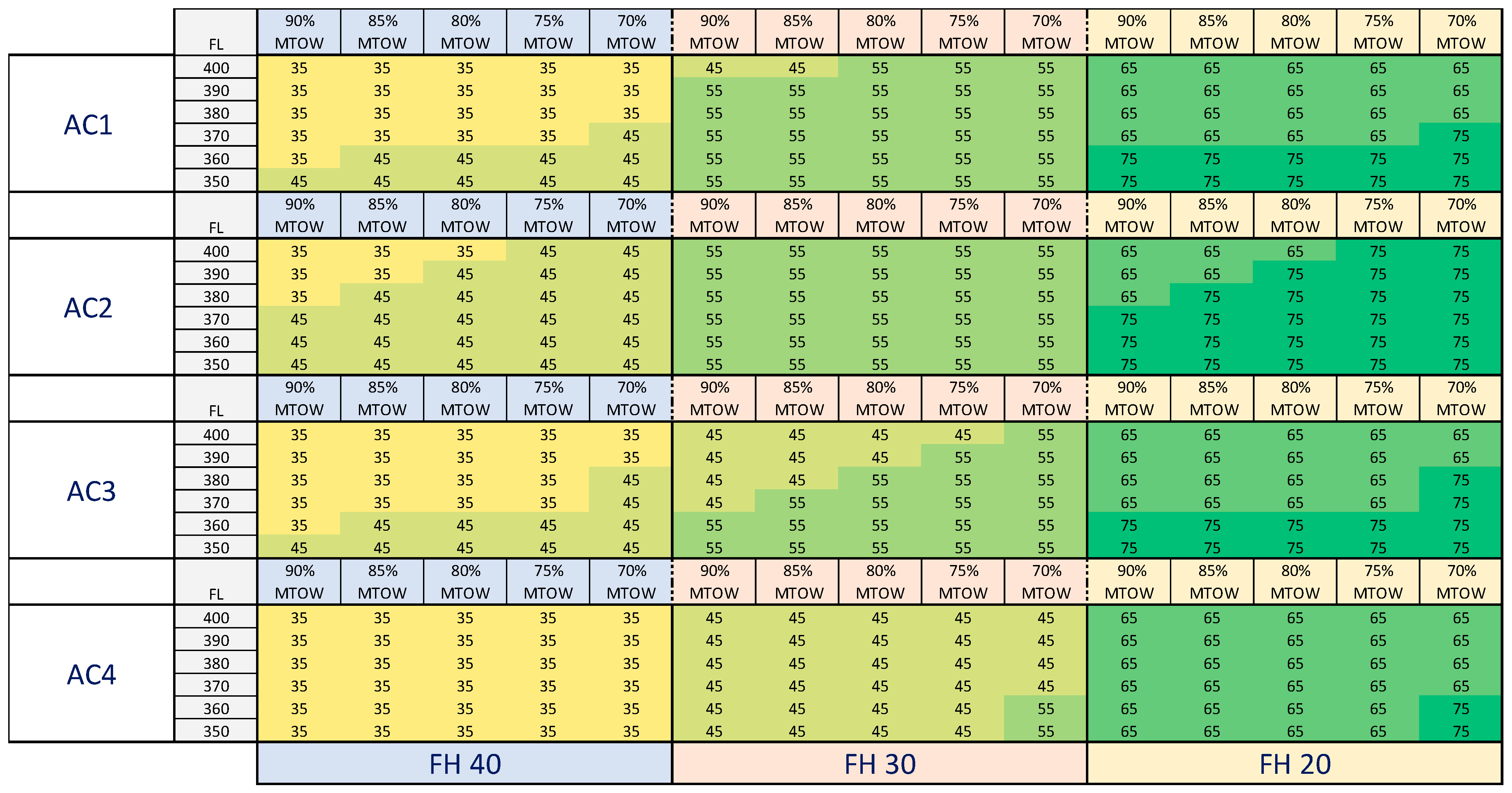
Figure A3 shows the results for the unconstrained descent AM obtained for the TCPA calculated for a minimum separation value of 5 NM.
Figure A3.
Descent AM results, unconstrained ROD. TCPA 5 NM.

- TCPA–4 NM
Figure A4 shows the results for the climb AM obtained for the TCPA calculated for a minimum separation value of 4 NM.
Figure A4.
Climb AM results. TCPA 4 NM.

Figure A5 shows the results for the descent AM obtained with an ROD limited to 1500 ft/min for the TCPA calculated for a minimum separation value of 4 NM.
Figure A5.
Descent AM results, ROD limited to 1500 ft/min. TCPA 4 NM.

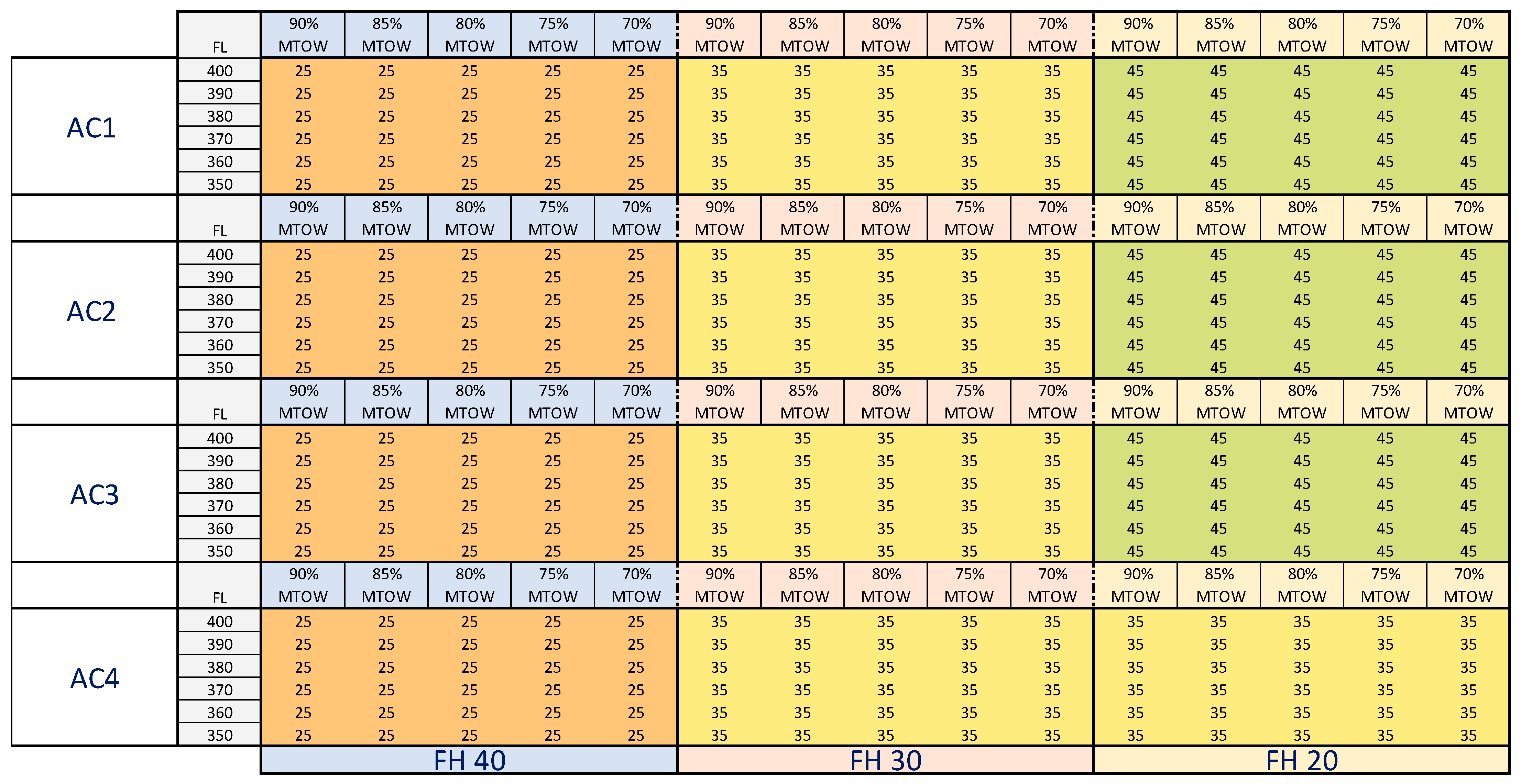
Figure A6 shows the results for the unconstrained descent AM obtained for the TCPA calculated for a minimum separation value of 3 NM.
Figure A6.
Descent AM results, unconstrained ROD. TCPA 4 NM.

- TCPA–3 NM
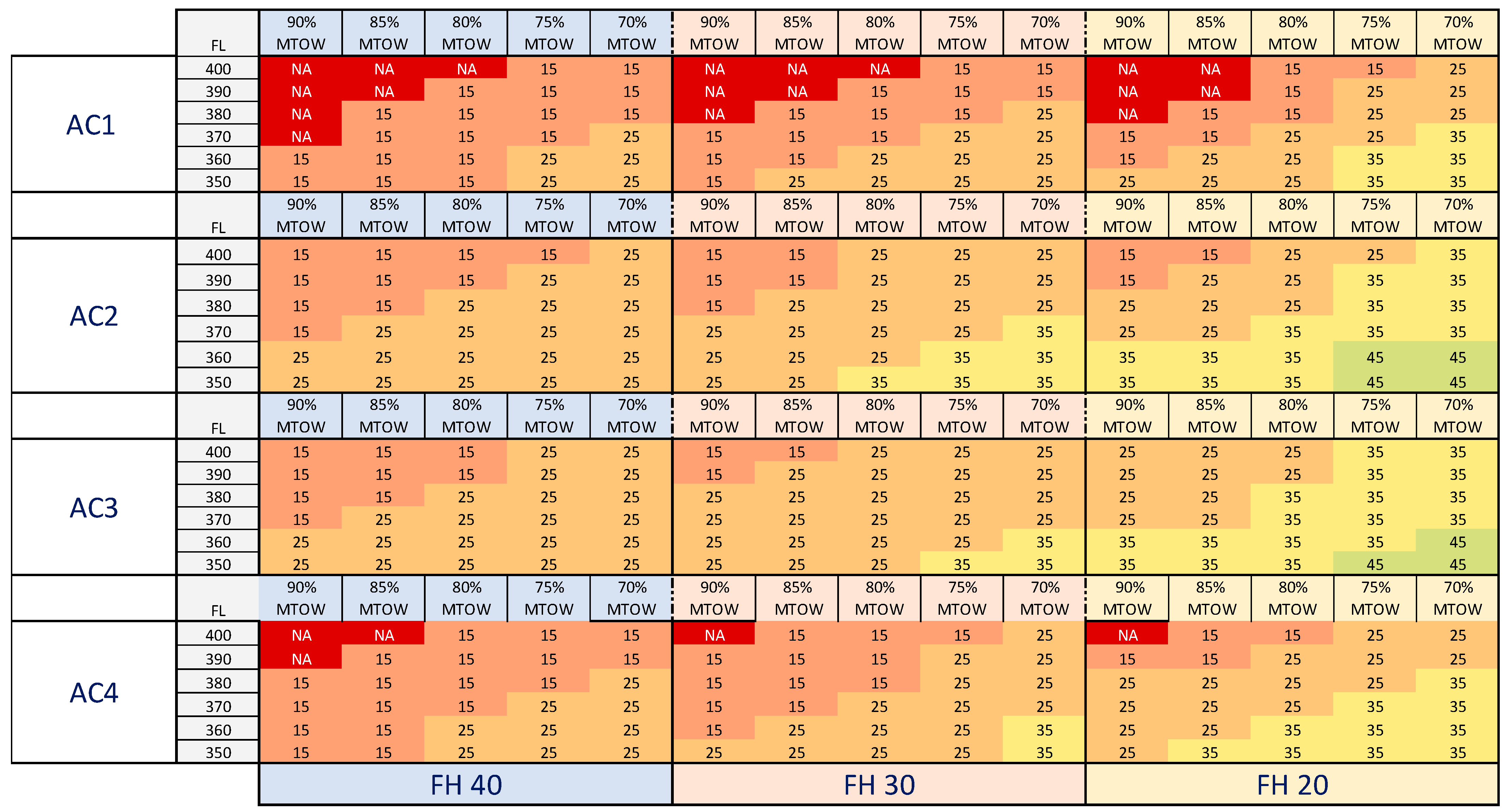
Figure A7 shows the results for the climb AM obtained for the TCPA calculated for a minimum separation value of 3 NM.
Figure A7.
Climb AM results. TCPA 3 NM.

Figure A8 shows the results for the descent AM obtained with an ROD limited to 1500 ft/min for the TCPA calculated for a minimum separation value of 3 NM.
Figure A8.
Descent AM results, ROD limited to 1500 ft/min. TCPA 3 NM.

Figure A9 shows the results for the unconstrained descent AM obtained for the TCPA calculated for a minimum separation value of 3 NM.
Figure A9.
Descent AM results, unconstrained ROD. TCPA 3 NM.

References
- EUROCONTROL. EUROCONTROL Forecast Update 2023–2029 Report. Available online: https://www.eurocontrol.int/publication/eurocontrol-forecast-update-2023-2029 (accessed on 2 April 2023).
- Reynolds, T.G.; Hansman, R.J. Analysis of separation minima using a surveillance state vector approach. In Proceedings of the 3rd USA/Europe Air Traffic Management R&D Seminar, Napoli, Italy, 13–16 June 2000; pp. 13–16. [Google Scholar]
- EUROCONTROL. Guidelines for the Application of the ECAC Radar Separation Minima. 1998. Available online: http://www.eurocontrol.int/sites/default/files/publication/content/documents/nm/ecac_radar_sep_min.pdf (accessed on 30 November 2022).
- Maroto, M.P.; García-Heras, J.; Sanz, L.P.; Serrano-Mira, L.; Pérez-Castán, J.A. Performance Impact Assessment of Reducing Separation Minima for En-Route Operations. Aerospace 2022, 9, 772. [Google Scholar] [CrossRef]
- EUROCONTROL. ‘RECAT-EU’ European Wake Turbulence Categorisation and Separation Minima on Approach and Departure Edition Number: 1.2 Edition. 2018. Available online: https://www.eurocontrol.int/sites/default/files/2021-07/recat-eu-released-september-2018.pdf (accessed on 10 October 2022).
- EUROCONTROL. EUROCONTROL Guidelines on Time-Based Separation (TBS) for Final Approach. Available online: https://www.eurocontrol.int/publication/eurocontrol-guidelines-time-based-separation-tbs-final-approach (accessed on 3 February 2023).
- NATS. Time Based Separation (TBS) for Pilots Flying into Heathrow. NATS Fact Sheet. Available online: /https://www.nats.aero/wp-content/uploads/2014/12/TBS-Crew-Fact-Sheet1.pdf (accessed on 3 February 2023).
- NATS. Enhanced Time Based Separation (eTBS). Available online: https://www.nats.aero/wp-content/uploads/2017/03/Full_eTBS_PresentationV1.pdf (accessed on 3 February 2023).
- ICAO. Performance-Based Navigation (PBN) Manual; ICAO: Montreal, QC, Canada, 2020. [Google Scholar]
- Netjasov, F. Framework for airspace planning and design based on conflict risk assessment. Part 1: Conflict risk assessment model for airspace strategic planning. Transp. Res. Part C Emerg. Technol. 2012, 24, 190–212. [Google Scholar] [CrossRef]
- Reich, P.G. Analysis of Long-Range Air Traffic Systems: Separation Standards—I. J. Navig. 1997, 50, 436–447. [Google Scholar] [CrossRef]
- Reich, P.G. Analysis of long-range air Separation Standards—II. J. Navig. 1966, 19, 169–186. [Google Scholar] [CrossRef]
- Reich, P.G. Analysis of long-range air traffic systems: Separation standards—III. J. Navig. 1997, 50, 436–446. [Google Scholar] [CrossRef]
- Machol, R.E. An Aircraft Collision Model. Manag. Sci. 1975, 21, 1089–1101. [Google Scholar] [CrossRef]
- Hsu, D.A. The Evaluation of Aircraft Collision Probabilities at Intersecting Air Routes. J. Navig. 1981, 34, 78–102. [Google Scholar] [CrossRef]
- Anderson, D.; Lin, X.G. A Collision Risk Model for a Crossin Track Separation Methodology. J. Navig. 1996, 49, 337–349. [Google Scholar] [CrossRef]
- ICAO. A Unified Framework for Collision Risk Modelling in Support of the Manual on Airspace Planning Methodology for the Determination of Separation Minima (Doc 9689); ICAO: Montreal, QC, Canada, 2009. [Google Scholar]
- ICAO. Manual on Airspace Planning Methodology for the Determination of Separation Minima; ICAO: Montreal, QC, Canada, 1998; p. 3. [Google Scholar]
- Brooker, P. Radar Inaccuracies and Mid-Air Collision Risk: Part 2 En Route Radar Separation Minima. J. Navig. 2004, 57, 39–51. [Google Scholar] [CrossRef]
- Nieto, F.J.S.; Valdés, R.A.; González, E.J.G.; McAuley, G.; Izquierdo, M.I. Development of a three-dimensional collision risk model tool to assess safety in high density en-route airspaces. Proc. Inst. Mech. Eng. Part G J. Aerosp. Eng. 2010, 224, 1119–1129. [Google Scholar] [CrossRef] [Green Version]
- Bakker, G.J.; Blom, H.A.P. Air traffic collision risk modeling. Proc. IEEE Conf. Decis. Control 1993, 2, 1464–1469. [Google Scholar] [CrossRef]
- Blom, H.; Bakker, B.; Everdij, M.; Van Der Park, M. Collision risk modeling of air traffic. In Proceedings of the European Control Conference, ECC 2003, Cambridge, UK, 1–4 September 2003; pp. 2236–2241. [Google Scholar] [CrossRef]
- Barnett, A. Free-Flight and en Route Air Safety: A First-Order Analysis. Oper. Res. 2000, 48, 833–845. [Google Scholar] [CrossRef]
- Ennis, R.L.; Zhao, Y.J. A Formal Approach to the Analysis of Aircraft Protected Zone. Air Traffic Control Q. 2004, 12, 75–102. [Google Scholar] [CrossRef] [Green Version]
- Thompson, S.D. Terminal Area Separation Standards: Historical Development, Current Standards, and Processes for Change; Massachusetts Inst of Tech Lexington Lincoln Lab: Lexington, MA, USA, 1997. [Google Scholar]
- Thompson, S.D.; Flavin, J.M. Surveillance Accuracy Requirements in Support of Separation Services. Linc. Lab. J. 2006, 16, 1. [Google Scholar]
- Thompson, S.D.; Andrews, J.W.; Harris, G.S.; Sinclair, K.A. Required Surveillance Performance Accuracy to Support 3-Mile and 5-Mile Separation in the National Airspace System; MIT Lincoln Laboratory: Lexington, MA, USA, 2006. [Google Scholar]
- EUROCONTROL. EUROCONTROL Specification for ATM Surveillance System Performance (Volume 1). Available online: https://www.eurocontrol.int/publication/eurocontrol-specification-atm-surveillance-system-performance-esassp (accessed on 16 September 2022).
- EUROCONTROL. EUROCONTROL Specification for ATM Surveillance System Performance (Volume 2 Appendices). Available online: https://www.eurocontrol.int/publication/eurocontrol-specification-atm-surveillance-system-performance-esassp (accessed on 16 September 2022).
- Safety, Performance and Interoperability Requirements Document for Ads-B-Rad Application; Document ED–161; EUROCAE: Malaoff, France, September 2009.
- ICAO. Doc 9854, Global Air Traffic Management Operational Concept; ICAO: Montreal, QC, Canada, 2005; p. 82. [Google Scholar]
- Pérez-Castán, J.A.; Pérez-Sanz, L.; Serrano-Mira, L.; Saéz-Hernando, F.J.; Gauxachs, I.R.; Gómez-Comendador, V.F. Design of an ATC Tool for Conflict Detection Based on Machine Learning Techniques. Aerospace 2022, 9, 67. [Google Scholar] [CrossRef]
- Serrano-Mira, L.; Maroto, M.P.; Ayra, E.S.; Pérez-Castán, J.A.; Liang-Cheng, S.Z.Y.; Arias, V.G.; Pérez-Sanz, L. Identification and Quantification of Contributing Factors to the Criticality of Aircraft Loss of Separation. Aerospace 2022, 9, 513. [Google Scholar] [CrossRef]
- Netjasov, F.; Vidosavljevic, A.; Tosic, V.; Everdij, M.H.; Blom, H.A. Development, validation and application of stochastically and dynamically coloured Petri net model of ACAS operations for safety assessment purposes. Transp. Res. Part C Emerg. Technol. 2013, 33, 167–195. [Google Scholar] [CrossRef]
- Coulter, D.M. UAS Integration into the National Airspace System: Modeling the Sense and Avoid Challenge. In Proceedings of the AIAA Infotech@Aerospace Conference, Seattle, WA, USA, 6–9 April 2009. [Google Scholar]
- Askelson, M.; Cathey, H.; ASSURE-FAA. Small UAS Detect and Avoid Requirements Necessary for Limited Beyond Visual Line of Sight (BVLOS) Operations; Aviation Faculty Publications; JDOSAS, University of North Dakota, Grand Forks and Physical Science Laboratory, New Mexico State University: Las Cruces, NM, USA, 2017. [Google Scholar]
- Shively, R.J.; Vu, K.P.L.; Buker, T.J. Unmanned aircraft system response to air traffic control clearances: Measured response. In Proceedings of the Human Factors and Ergonomics Society, Perth, Australia, 2–4 December 2013; pp. 31–35. [Google Scholar] [CrossRef] [Green Version]
- Stelzer, E.K.; Morgan, C.E.; Mcgarry, K.A.; Klein, K.A.; Kerns, K. Human-in-the-Loop Simulations of Surface Trajectory-Based Operations: An Evaluation of Taxi Routing and Surface Conformance Monitoring Decision Support Tool Capabilities. In Proceedings of the Ninth USA/Europe Air Traffic Management Research and Development Seminar, ATM2011, Berlin, Germany, 14–17 June 2011. [Google Scholar]
- Cardosi, K.M.; Boole, P.W.; Volpe, J.A. AD-A242 527—Analysis of Pilot Response Time to Time-Critical Air Traffic Control Calls; John A Volpe National Transportation Systems Center: Cambridge, MA, USA, 1991. [Google Scholar]
- EUROCONTROL. DNV Technical, Hazard Analysis of Route Separation Standards; EUROCONTROL: Brussels, Belgium, 1997. [Google Scholar]
- EUROCONTROL. User Manual for the Base of Aircraft Data (BADA). Available online: https://www.eurocontrol.int/publication/user-manual-base-aircraft-data-bada (accessed on 10 June 2022).
- EUROCONTROL. ACAS Guide Airborne Collision Avoidance Systems. 2022. Available online: https://www.eurocontrol.int/publication/airborne-collision-avoidance-system-acas-guide (accessed on 11 January 2023).
- Airbus. Flight Operations Briefing Notes. Approach Techniques. Aircraft Energy Management during Approach; Airbus: Blagnac, France, 2005. [Google Scholar]
- EASA. Easy Access Rules for Large Aeroplanes(CS-25) (Amendment 27) Report; EASA: Cologne, Germany, 2023.
- Lejarza, J.; Lejarza, I. Distribución Normal; Universidad de Valencia: Valencia, Spain, 2010. [Google Scholar]
- ICAO. Doc 4444. Air Traffic Management. PANS-ATM; ICAO: Montreal, QC, Canada, 2016. [Google Scholar]
- Gallego, C.E.V.; Javier, F.; Nieto, S. Discussion on Complexity and TCAS Indicators for Coherent Safety Net Transitions. In Proceedings of the SESAR Innovations Days (SIDs), Delft, The Netherlands, 8–10 November 2016. [Google Scholar]
Figure 1.
Trajectory prediction by SMT.

Figure 2.
SMT architecture and relation to the working position of the ATCo.

Figure 3.
Barrier diagram for mid-air collisions (MAC), IRP model.

Figure 4.
Diagram of Necessary time and Available Time in the short time horizon to collision.

Figure 5.
Scenario simulated for determining .

Figure 6.
Necessary time based on Encounter Timeline concept.

Figure 7.
Climb and descent avoidance maneuvers.

Figure 8.
(a) Change in ROC with FL for different aircraft. (b) Change in ROC with aircraft weight for a specific FL.
Figure 8.
(a) Change in ROC with FL for different aircraft. (b) Change in ROC with aircraft weight for a specific FL.

Figure 9.
Climb AM performed by the maneuvering AC simulated in MATLAB. Overview and profile view.

Figure 10.
Descent AM performed by the maneuvering AC simulated in MATLAB. Overview and profile view.
Figure 10.
Descent AM performed by the maneuvering AC simulated in MATLAB. Overview and profile view.

Figure 11.
Engine response [43].
Figure 11.
Engine response [43].

Figure 12.
Evolution of TCPA with intersection angle and separation minima.

Figure 13.
(a) Distance evolution between aircraft for different angles; (b) Closing speed rate for different angles.
Figure 13.
(a) Distance evolution between aircraft for different angles; (b) Closing speed rate for different angles.

Figure 14.
AC 1, AC 2, AC 3, AC 4 for a Climb AM at different FL and weight.


Figure 15.
AC 1, AC 2, AC 3, AC 4 for a Descent AM with unconstrained ROD at different FL and weight.
Figure 15.
AC 1, AC 2, AC 3, AC 4 for a Descent AM with unconstrained ROD at different FL and weight.

Figure 16.
TCPA variation with separation minima.

Figure 17.
TCPA variation in encounters with MM aircraft, MH and HH aircraft.

Figure 18.
Maximum possible angle between tracks: Climb AM results, HF 40 s. TCPA 5 NM.


Table 1.
Control variables of the simulations.
| BADA Worst-Case Scenario Simulations | |
|---|---|
| Aircraft that executes the AM | Maneuvering aircraft |
| Kind of maneuvers for collision avoidance | Climb, Descent |
| Aircraft models considered | AC1(M), AC2(M), AC3(M), AC4(H) |
| Aircraft weights considered | 0.9 MTOW, 0.85 MTOW, 0.8 MTOW, 0.75 MTOW, 0.7 MTOW |
| Flight levels considered | FL350, FL360, FL370, FL380, FL390, FL400 |
| Intersection angles considered | 15°, 25°, 35°, 45°, 55°, 65°, 75°, 85°, 95°, 105°, 115°, 125°, 135°, 145°, 155°, 165°, 175° |
Table 2.
Climb AM parameters for different aircraft.
| Maneuvering Aircraft | FL [-] | Mach Cruise [-] | Weight (0.75 MTOW) [kg] | Thrust [N] | Drag [N] | ROC [ft/min] | Wake Turbulence Category |
|---|---|---|---|---|---|---|---|
| AC 1 | 360 | 0.78 | 57,750 | 53,107 | 41,851 | 915 | M |
| AC 2 | 360 | 0.78 | 52,560 | 52,902 | 36,693 | 1447 | M |
| AC 3 | 360 | 0.78 | 52,500 | 51,168 | 36,283 | 1331 | M |
| AC 4 | 360 | 0.82 | 172,500 | 136,920 | 97,121 | 1140 | H |
Table 3.
Descent AM parameters for different aircraft.
| Maneuvering Aircraft | FL [-] | Mach Descent [-] | Weight (0.8 MTOW) [kg] | Thrust [N] | Drag [N] | ROD [ft/min] | Wake Turbulence Category |
|---|---|---|---|---|---|---|---|
| AC 1 | 380 | 0.79 | 61,600 | 6785 | 42,040 | 2644 | M |
| AC 2 | 380 | 0.78 | 56,064 | 1797 | 36,598 | 2868 | M |
| AC 3 | 380 | 0.79 | 56,000 | 4007 | 35,472 | 2596 | M |
| AC 4 | 380 | 0.82 | 184,000 | 9038 | 97,588 | 2337 | H |
Disclaimer/Publisher’s Note: The statements, opinions and data contained in all publications are solely those of the individual author(s) and contributor(s) and not of MDPI and/or the editor(s). MDPI and/or the editor(s) disclaim responsibility for any injury to people or property resulting from any ideas, methods, instructions or products referred to in the content. |
© 2023 by the authors. Licensee MDPI, Basel, Switzerland. This article is an open access article distributed under the terms and conditions of the Creative Commons Attribution (CC BY) license (https://creativecommons.org/licenses/by/4.0/).
Share and Cite
MDPI and ACS Style
Serrano-Mira, L.; Sanz, L.P.; Pérez-Castán, J.A.; Netjasov, F.; Moreno, I.G.; Ayra, E.S. Preliminary Feasibility Study of the Ad Hoc Separation Operational Concept. Aerospace 2023, 10, 539. https://doi.org/10.3390/aerospace10060539
AMA Style
Serrano-Mira L, Sanz LP, Pérez-Castán JA, Netjasov F, Moreno IG, Ayra ES. Preliminary Feasibility Study of the Ad Hoc Separation Operational Concept. Aerospace. 2023; 10(6):539. https://doi.org/10.3390/aerospace10060539
Chicago/Turabian StyleSerrano-Mira, Lidia, Luis Pérez Sanz, Javier A. Pérez-Castán, Fedja Netjasov, Irene García Moreno, and Eduardo S. Ayra. 2023. "Preliminary Feasibility Study of the Ad Hoc Separation Operational Concept" Aerospace 10, no. 6: 539. https://doi.org/10.3390/aerospace10060539
Note that from the first issue of 2016, this journal uses article numbers instead of page numbers. See further details here.