

Data-Driven Modeling of Air Traffic Controllers’ Policy to Resolve Conflicts


University of Piraeus Research Center, Department of Digital Systems, University of Piraeus, 18534 Piraeus, Greece
*
Author to whom correspondence should be addressed.
Aerospace 2023, 10(6), 557; https://doi.org/10.3390/aerospace10060557
Submission received: 5 May 2023
/
Revised: 7 June 2023
/
Accepted: 9 June 2023
/
Published: 13 June 2023
(This article belongs to the Collection Air Transportation—Operations and Management)
Abstract
:With the aim to enhance automation in conflict detection and resolution (CD&R) tasks in the air traffic management (ATM) domain, this article studies the use of artificial intelligence and machine learning (AI/ML) methods to learn air traffic controllers’ (ATCOs) policy in resolving conflicts among aircraft assessed to violate separation minimum constraints during the en route phase of flights, in the tactical phase of operations. The objective is to model conflicts are being resolved by ATCOs. Towards this goal, the article formulates the ATCO policy learning problem for conflict resolution, addresses the challenging issue of an inherent lack of information in real-world data, and presents AI/ML methods that learn models of ATCOs’ behavior. The methods are evaluated using real-world datasets. The results show that AI/ML methods can achieve good accuracy on predicting ATCOs’ actions given specific conflicts, revealing the preferences of ATCOs for resolution actions in specific circumstances. However, the high accuracy of predictions is hindered by real-world data-inherent limitations.
1. Introduction
Different initiatives worldwide, such as NextGen [1] in the US and SESAR [2] in Europe, have been investigating the implementation of automation to enhance the efficiency and cost-effectiveness of the air traffic management (ATM) system, which is due to the need to increase the airspace capacity, and thus the density and complexity of traffic. Air traffic control (ATC) in the air traffic management (ATM) domain, according to International Civil Aviation Organization (ICAO) Annex 11 [3], is “a service provided for the purpose of: (a) preventing collisions: (1) between aircraft, and (2) on the maneuvering area between aircraft and obstructions; and (b) expediting and maintaining an orderly flow of air traffic”. The provision of safe ATC services determines traffic volume, which must not exceed the capacities declared. However, capacities should be utilized to the maximum extent due to increased demand and the need for the optimal utilization of resources, without compromising the efficiency and safety of flights. This trade-off introduces challenging issues in the aviation industry, where artificial intelligence and machine learning (AI/ML) can provide solutions.
To maintain safety and prevent collisions between aircraft—a consequence of increased traffic—the ATM system imposes specific separation minima constraints between aircraft, both at the horizontal and vertical axes. When surveillance systems are used, the minimum required horizontal separation is 5 NM and the vertical minimum separation is 1000 ft (300 m) below Flight Level (FL) 290, and 2000 ft (600 m) from FL290 and above. The Air Traffic Service (ATS) authority may reduce or increase the separation minima based on the surveillance systems’ capabilities, and situations between aircraft [4].
A loss of separation is defined as the violation of separation minima in controlled airspaces, whereas a conflict is defined as a predicted violation of the separation minima.
As described in [5], tactical conflict detection and resolution (CD&R) is executed by Executive Controllers (ECs). These are air traffic controllers (ATCOs) who detect and resolve conflicts in their respective sectors, which are their Areas of Responsibilities (AoRs). The resolution of conflicts happens in coordination with downstream sectors, so as not to increase traffic in these sectors. In a flight-centric ATC, such as the one considered in this article, the detection and resolution of conflicts may happen independently from sectors, while sectors can provide further spatio-temporal constraints regarding areas of responsibility, which in the general case can be of any granularity.
To resolve conflicts at the tactical phase of operations, ATCOs issue instructions regarding changes in the flight trajectory, given (a) the trajectory up to a specific time point, (b) predictions of the evolution of the trajectory from that time point and on, and (c) the evolution of conflicts due to traffic. Trajectory prediction is crucial to detecting conflicts, but the uncertainty of the prediction, together with the error in prediction, grows as the prediction horizon grows. This implies uncertainties in the assessment of conflicts, as well as uncertainties in the resolution of conflicts.
As a conclusion, the detection and the resolution of conflicts (i.e., the CD&R task) involves human expertise and informed judgment. Thus, it is very difficult to hand-craft criteria which will drive a system to decide whether a conflict deserves a certain reaction at a particular time point and what the best reaction is (i.e., the one that resolves the conflict in the most efficient way and with high probability), especially in long-term horizons (i.e., beyond 15–20 min).
This work contributes to automating the resolution of conflicts as part of the ATC (https://www.skybrary.aero/articles/air-traffic-control-service, accessed on 12 June 2023) service, during the en route phase of flights, promoting the safe, orderly and expeditious flow of air traffic at the tactical phase of operations, modeling ATCOs’ behavior to resolve conflicts.
Our conjecture is that in safety-critical domains such as ATC, the actions proposed by automated systems in specific circumstances should be similar to the actions decided and applied by humans. The authors in [6] show that actions adhering to the operator’s preferences increase the acceptance rate of the system’s proposed actions and decrease workload. This has important implications in the automation process, taking into account human expertise, as well as human-like flexibility and tolerance in reacting to situations. Indeed, based on these, we believe that by modeling the reactions of ATCOs we can build models that promote efficacy and trust for automated systems. Decisions that adhere to human reasoning, preferences and objectives can be made more understandable and intuitively transparent to human operators. This does not imply that explainability/transparency is not necessary in this case, but this is not within the scope of this article.
Specifically, this article reports on data-driven AI/ML methods to model the ATCOs’ behavior. Modeling the ATCOs’ behavior, as also proposed in [7], implies learning the ATCOs react to resolve a detected conflict, and they react. This work formulates the problem of modeling the ATCO policy, specifying the ATCOs react to resolve conflicts by issuing specific instructions in specific conflicting situations. This, in conjunction with predicting the ATCOs react to resolve a conflict, as is carried out in [7], paves the way to (a) automating the ATC process, and (b) optimizing the ATC process with respect to ATCOs’ preferences and modes of behavior, ensuring enhanced decision making for ATCOs, while leveraging (c) human–AI collaboration in the context of ATC.
1.1. Related Work
In recent years, numerous studies have explored the challenge of automating the conflict detection and resolution (CD&R) task, or developing decision support tools to assist ATCOs in performing the CD&R task. A survey of CD&R for manned and unmanned aviation is presented in [8]. The authors in [9] present a method for addressing strategic planning that involves traffic on a continent scale. The proposed method utilizes a hybrid metaheuristic optimization algorithm that combines the benefits of simulated annealing and hill-climbing local search methods, to determine an optimal de-conflicted route and departure time for each flight.
The authors in [10] address the problem of resolving conflicts at the tactical phase of operations by using a nature-inspired light propagation algorithm that generates conflict-free 4D trajectories. In [11], the authors present a genetic algorithm-based approach to perform conflict resolution during the en route phase of flights and in the tactical phase of operations, while in [12], the authors resolve conflicts using a lattice-based search space exploration method. The work presented in [13] predicts the evolution of trajectories at the pre-tactical phase based on historical trajectories and weather observations by utilizing a Hidden Markov Model (HMM). The predictions made are used to detect conflicts and assess the probabilities of states related to conflicts. The authors use a variant of the Viterbi algorithm to apply resolution actions to flights.
The use of reinforcement learning (RL) techniques to address the CD&R task has attracted significant interest in recent years. A deep deterministic policy gradient (DDPG)-based approach is used in [14,15] to resolve conflicts between two aircraft in the presence of uncertainty. In [16], CD&R is formulated as a multi-agent reinforcement learning problem, which is solved by a message-passing actor critic model. In [17], the authors combine kernel-based RL with deep multi-agent reinforcement learning (MARL) to resolve conflicts by applying speed changes in real time, also considering other factors such as fuel consumption and airspace congestion. The authors in [18] use a multi-agent deep deterministic policy gradient (MADPG) to resolve conflicts, also considering time, fuel consumption and airspace complexity.
In contrast to the above-mentioned approaches, and closer to our approach, are the methods that somehow consider the ATCOs’ preferences, either in a data-driven way as in [19,20,21], or by using rules and procedures derived from human experts as in [22].
In [19], the authors present a conflict resolution approach that operates at the strategic phase of operations. This work presents a data-driven model that (a) classifies the conflict resolution maneuvers by considering the relationship between the conflicting aircraft and (b) clusters the conflict resolution actions in order to discretize them. The centroid of each cluster is used as a possible solution. Next, an -constrained multi-objective optimization method is used to find the Pareto-optimal solutions that minimize the fuel consumption and maximize the likelihood of ATCOs to issue a resolution action.
A conflict resolution advisory system that incorporates human preferences is presented in [20]. To gather resolution actions assigned by humans, the authors utilize an interactive conflict solver. Then, the proposed methodology trains an RL agent to resolve conflicts while considering the characteristics of the resolution actions assigned by humans. This work does not use historical ATCO resolution actions and focuses on the turning point maneuver, deciding the trajectory change point (TCP), i.e., the point at which an aircraft will turn towards its initial track, after changing its heading to resolve a conflict. In contrast to predicting resolution actions issued by ATCOs, here, the authors focus on how the ATCOs will guide the aircraft to perform a TCP maneuver.
In [21], the authors present a method suggesting personalized resolution actions to ATCOs. To do so, they train a convolutional neural network (NN) on individual controller’s data. The data are gathered during human-in-the-loop simulations, where humans assign resolution actions to solve conflicts. The data used in this study contain solution space diagrams (SSD), which integrate different features that are critical for the CD&R problem. To collect ATCOs’ resolution actions, the authors created synthetic traffic scenarios inspired by real-world traffic flows. These were presented to non-experts (university staff and students), which solved the conflicts. Resolution actions issued by the participants were recorded and used to train the convolutional NN.
In [22], the authors present a method that proposes 4D conflict resolution trajectories. To resolve conflicts efficiently, the authors use rules and procedures provided by human experts, operational insights and analytical studies. This is different from our approach, where we model the ATCOs’ behavior as it is revealed by the historical ATCO events.
In our previous work [7], we considered the problem of modeling the ATCOs’ reactions in the presence of conflicts, focusing on predicting whether and when the ATCOs will react in the presence of a conflict. Here, our aim is to predict how ATCOs will react in situations with conflicts, predicting the resolution action the ATCOs will instruct. To achieve this, we formulate the ATCO policy modeling problem in a data-driven way, and we propose AI/ML techniques to learn models of ATCO policy in resolving conflicts, exploiting data recording ATCO events (i.e., conflict resolution actions issued at specific time points) and historical flight trajectories. This implies learning models that predict which resolution action the ATCOs will instruct, according to demonstrated conflict resolution actions.
In contrast to the data-driven methods mentioned above, this work advances the state of the art in CD&R automation, formulating and addressing the problem of imitating the ATCOs behavior, thus closing the gap between automation in CD&R and ATCOs.
1.2. Contributions
Casting CD&R as a data-driven supervised machine learning problem from the perspective of imitating ATCOs behavior is novel, since, as far as we know, there is not any other work that does so, exploiting real-world data comprising demonstrated historical flight trajectories annotated with ATCO events. Indeed, as discussed in the related work section, most of the CD&R approaches are trained, validated and tested in simulated settings where agents, representing aircraft, learn by interacting with their environment without considering the ATCO policy.
Complementing our efforts towards imitating ATCOs, described in [7], the objective here is to predict the ATCOs will react in specific circumstances, in case they decide to react.
The specific contributions made in this article are as follows:
- It specifies the problem of learning the ATCO policy as a supervised imitation learning task. Considering specific types of resolution actions that may be applied in the en route phase of flights at the tactical phase of operations, this results in a classification task.
- It studies alternative AI/ML methods to learn models of ATCOs’ behavior with respect to the formulation proposed.
- It evaluates the proposed AI/ML methods using real-world data, addressing the challenges to imitating ATCOs adequately.
It must be noted that, ideally, learning the ATCO policy problem through a data-driven learning process necessitates having data of the conflicting situations that occurred and motivated the recorded ATCO resolution actions. These observations are not included in the historical dataset, which includes only the flight trajectories after the execution of the resolution actions. Therefore, to imitate ATCOs adequately, we need to reveal the conflicting situations that occurred. This is in contrast to detecting conflicts. This work exploits historical data to assess conflicts that may have occurred, and which caused the ATCOs’ reactions. This is a rather challenging issue that is addressed and discussed in this article.
The article is structured as follows: Section 2 presents the proposed methodological steps and the AI/ML methods used for solving the problem. Section 3 presents the experimental results. Section 4 provides a thorough discussion of the results and challenges, and finally, Section 5 concludes the article and presents future work.
2. Materials and Methods
2.1. Problem Specification
This section starts with some definitions regarding domain terms, and then proceeds to specify the ATCO policy modeling problem.
2.1.1. Definitions
A is defined as a sequence of states ordered in time: .
As the ATCO policy should be agnostic to the specific spatio-temporal (longitude, latitude, altitude, and timestamp) position of an aircraft, to generalize beyond specific conflicting situations with various aircraft relative positions, areas, and flight origin–destination pairs, models should use states = 〈, 〉, , where specifies aircraft state features—other than positional—that are relevant to the CD&R task, and is restricted to observations regarding conflicts. This is very important to modeling the ATCO policy, as also presented in Section 2.2.2.
The predicted trajectory indicates the future evolution of the aircraft state with respect to (a) the current flight conditions (e.g., an initial state with co-occurring trajectories according to flight plans or other predictions, weather conditions etc.), (b) predictions of contextual features (e.g., weather forecast at specific points/regions, or predicted trajectories of other aircraft), and (c) a policy specifying the trajectory’s evolution, i.e., how the aircraft transitions between states, starting from the current state and on.
The evolution of a trajectory T, from time point t up to , is denoted . A predicted trajectory from t to is denoted as . A set of such predictions, showing the potential trajectory evolution of , is denoted by .
Regarding the assessment of conflicts between aircraft trajectories, the position of an aircraft i when the distance between i and another aircraft j is at its minimum is called the Closest Point of Approach (CPA) (https://www.skybrary.aero/index.php/Closest_Point_of_Approach_(CPA), accessed on 12 June 2023) of i with regard to j. We refer to the time at which the CPA occurs as the time at the CPA. In general, the CPA is computed in the horizontal or vertical axis or in all three dimensions. In this article we compute the CPA at the horizontal axis following the methodology presented in [15], while also considering the vertical distance at the CPA in order to detect potential conflicts.
The Crossing Point (CP) (https://www.skybrary.aero/index.php/Vectoring_Geometry, accessed on 12 June 2023) of a pair of aircraft is the point at which the tracks of the aircraft intersect. The track (https://www.skybrary.aero/index.php/Heading,_Track_and_Radial, accessed on 12 June 2023) of an aircraft is the projection of the aircraft trajectory on the surface of Earth.
We revisit CPA and CP in Section 2.2.2, with further details on features that are of interest to the CD&R task.
Considering a spatiotemporal area , we define as neighbor trajectories in SA those trajectories that co-occur in , satisfying the following set of constraints regarding their tracks, CPA and CP.
- The aircraft have not crossed the crossing point;
- The tracks of the aircraft cross in less than minutes;
- The horizontal distance at the CPA is less than ;
- The time to the CPA is less than ;
- Aircraft altitude difference at the current time point is less than ft.
As shown in Table 1, the parameter is the crossing time threshold, is the horizontal distance threshold between aircraft at the CPA, is the time to the CPA threshold, and is the vertical distance threshold. We set min, min, and NM. It must be noted that we use a large horizontal distance threshold at the CPA () of 15 NM, in order to include margins of error and uncertainty when estimating ATCOs’ observations, triggering their reactions. This has been proven successful in [7] given the lack of information regarding conflicts causing ATCO events in datasets.
As already pointed out, historical data should ideally indicate the observations perceived by ATCOs before applying a conflict resolution action. Such observations should provide the features that drove the application of a specific action instead of others in ATCOs’ repertoire of actions, and concern the current situation involving specific aircraft trajectories, the prediction of the evolution of the trajectories before the “intervention” of ATCOs, and the assessment of conflicts. However, the historical datasets that this work exploits, provided by the Spanish ATON (Automated NORVASE Takes) platform, indicate only the type of the resolution actions instructed by ATCOs (e.g., change speed), and not the actions in full detail (e.g., how speed has been changed and for how long), and the effects of ATCOs’ resolution actions (i.e., the conflict-free trajectory), but not the rationale behind them. This lack of information presents challenges to the training of AI/ML systems, since it necessitates recovering the important observations that the ATCOs perceived or assessed, driving their decision. This entails exploiting expert knowledge to assess traffic as the ATCOs would, reveal the potential conflicts the ATCOs might have observed, and associate these potential conflicts with the prescribed resolution actions. Revealing such conflicts from historical datasets is not a trivial task in the ATC domain, as (a) the evolution of the trajectories is uncertain and ATCO assessments and practices may vary due to various reasons; and (b) to ensure safety, even when the predicted horizontal distance between flights at the CPA exceeds the horizontal separation minimum, ATCOs allow margins of error in perceiving flights. These margins may not be so large as we assume here, but it must be emphasized that we do so in order to reveal what the ATCOs perceive prior to reaction (i.e., to associate potential conflicting situations with resolution actions). In addition to the above challenges, associating potential conflicting situations with ATCOs’ resolution actions may introduce noise in the training of AI/ML methods, given the uncertainty in determining which features of assessed conflicts are those that provided the rationale for the ATCOs’ actions. This issue is further discussed subsequently as the “labels noise” problem.
The set of neighbor trajectories includes aircraft trajectories that cross and are in conflict, as defined below.
There is at least one trajectory point at time point t in , and a trajectory point at time point t in , such that it holds that the 3D spatial points of and are in the spatial region of and the aircraft’s and satisfy the set of constraints .
In addition, given a specific (usually called “focal” or “own”) trajectory and the spatiotemporal area , we define the set of neighbor and thus conflicting trajectories to in at a specific time point t, denoted by , to be trajectories that (a) have at least one point close to the focal trajectory point at the time t, using a horizontal distance measure and with respect to a distance threshold , and that (b) satisfy the constraints . Formally:
There is a trajectory point at time point t in and a trajectory point at time point t in such that it holds that (a) the 3D spatial points of and are in the spatial region of , (b) , and (c) the aircraft’s and satisfy the set of constraints in }.
It must be noted that although the detection of conflicts is carried out using the aircraft CPA, the additional rules for the identification of neighbor trajectories allows (a) detecting conflicts that correspond to the recorded ATCO resolution actions, which are not explicitly provided in historical datasets, and (b) filtering out aircraft that might be in conflict, but are not considered by the ATCOs at a specific time point (e.g., because the time to CPA is large). Rules can be refined when datasets include further information on conflicts.
2.1.2. Modeling the ATCOs Policy
Given a set of historical trajectories and a set of historical ATCO conflict resolution actions (ATCO events) associated with trajectories in , our goal is to learn a model that imitates the ATCOs behavior in terms of these resolution actions.
As described in [7], the problem of ATCOs’ reaction prediction concerns predicting , , and ATCOs will react to conflicts involving a particular aircraft executing the (focal) trajectory , and aircraft flight trajectories in , given a spatial area of responsibility .
The ATCO reaction prediction problem involves (a) the detection of potential conflicts with identified trajectories in , (b) deciding the time point for issuing a resolution action, given the time points at which conflicts occur, and (c) deciding the resolution action to be applied at that time point, thus shaping the future evolution of the trajectory for resolving conflicts.
Therefore, in order to be able to imitate the behavior of the ATCOs given and , one should develop models that are capable of the following:
- Predicting at any trajectory point whether the ATCOs would issue a resolution action;
- Representing the ATCO policy, predicting the resolution action the ATCOs would decide, if any.
As already pointed out, while the work in [7] focuses on learning models of ATCOs’ timely reactions, stated in the first problem above, in this article we focus on the second problem.
Specifically, the problem of modeling the ATCO policy is about deciding at any time point how the ATCOs will react, i.e., what conflict resolution action will apply in a focal trajectory , given conflicts involving that trajectory and trajectories in .
As already discussed, ATCO events indicate the of conflict resolution action instructed, e.g., speed change, and do not indicate further details about the resolution action. The actual resolution action cannot be revealed from the available data sources, due to a lack of information regarding the evolution of the trajectories if no resolution action applies, in conjunction with the uncertainty of how the trajectory evolves. Therefore, the specific problem addressed here is about predicting, at any time point in the en route phase and in the tactical phase of operations, the type of conflict resolution action that ATCOs apply in (focal trajectory), given conflicts involving the trajectory and trajectories in .
Casting the imitation problem as a classification problem, conflicts are classified according to the type of ATCO resolution actions in a supervised way, according to demonstrated ATCO events. Here, the task does not take into account the evolution of the conflicts, but only the characteristics of the conflicts when they occur. This entails a major difference of the classification task from the “classical” ATCO imitation task: the classification task prescribes a resolution action as learned by demonstration samples, but without considering the effects of this action. This may provide limitations to the generalization abilities of the classification task, as it does not exploit the fact that in similar conflicting situations the most valuable actions are those that shape trajectories in ways similar to those demonstrated. Further work must address this important issue.
2.2. Learning the ATCOs Policy
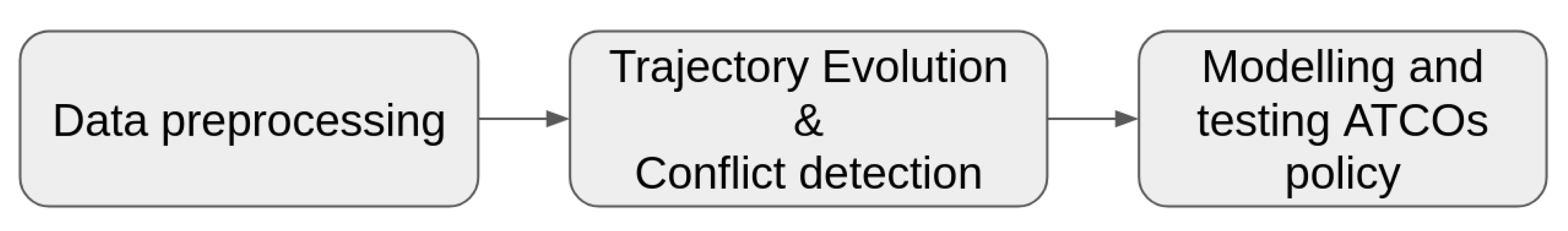
Figure 1 depicts the methodological steps proposed to learn the ATCO policy in a data-driven way.
The data pre-processing stage associates the available data sources of historical, flown, and thus conflict-free trajectories and ATCO events. The pre-processed datasets are used for training and testing the AI/ML models.
The trajectory evolution and conflict detection stage estimates for any trajectory T, at any time point t, including its potential evolution up to a time point , identifies potential neighbor trajectories within the area of responsibility (defined to have caused conflicts), and computes state features for the conflicts assessed to be associated with the historical ATCO events. (The data pre-processing and trajectory evolution and conflict detection stages are similar to those described in [7] but are repeated here for reasons of article conciseness.)
Finally, having detected potential conflicts associated with ATCO events, the ATCO policy models are trained and tested at the modeling and testing ATCO policy stage.
Subsequent sections present the data sources used, as well as each of the stages.
2.2.1. Data Sources
Exploited data sources include (a) historical surveillance data (IFS) from the Spanish ATC Platform SACTA (Automated System of Air Traffic Control), and (b) historical ATCO events about resolution actions that the ATCOs assigned to flights (ATON, Automated NORVASE Takes).
Surveillance data contain radar track points, which indicate the position of the aircraft (longitude, latitude, and altitude) and the timestamp, as well as information that allows the identification of flights, such as the callsign and the origin and destination airports.
The ATCO events dataset contains information related to conflict resolution actions assigned to flights by ATCOs. This identifies the flight (specifying the callsign and origin/destination airports), specifying the timestamp and the type of resolution action assigned to that flight:
<callsign, origin airport, destination airport, resolution action type>.
This information allows associating ATCO events (thus, resolution actions) with specific trajectory points.
In particular, an ATCO event for a resolution action () is associated with a trajectory (T) if the following conditions are met:
- .callsign = T.callsign
- .departure_airport = T.departure_airport
- .destination_airport = T.destination_airport
- Timestamp of the first T point ≤ timestamp of ≤ timestamp of the last T point.
Given that the above conditions hold for T and , the is associated with the trajectory point that is temporally closer to it.
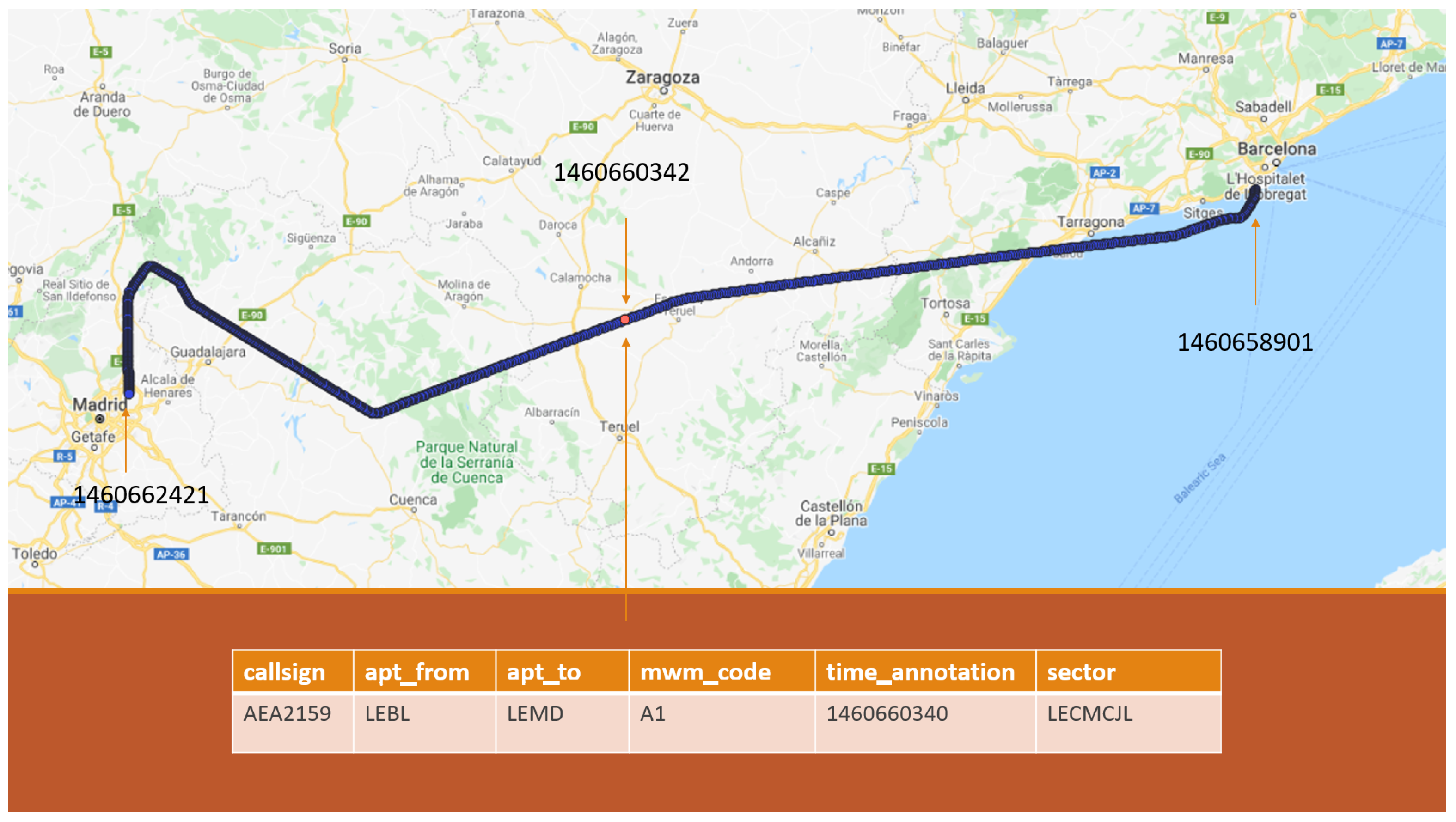
Figure 2 illustrates a case of associating an ATCO event with a trajectory. The table displays the attributes of the ATCO event, while the aircraft’s trajectory is represented by the blue line. The red point represents the trajectory point that is closest in time to the ATCO resolution action, along with its corresponding timestamp. Furthermore, the timestamp of the ATCO event is provided together with the timestamps of the first and last point of the trajectory.
2.2.2. Detection of Conflicts, States, and ATCOs’ Resolution Actions
Addressing the ATCO policy modeling problem in a data-driven way, the training process necessitates having data associating ATCOs’ observations regarding conflicts with specific reactions. As pointed out, these observations are not recorded in a historical dataset. In this stage, we aim to reveal the conflicts that would occur if the ATCOs would not react at a time point t. It involves revealing the cases where a trajectory is in conflict with another trajectory and that are assessed to violate the separation minima according to estimated trajectory predictions, and .
To detect potential conflicts between trajectories, the CPA between pairs of flights is computed using the speed and course information included in the radar tracks. Then, the violation of separation minima is checked. The CPA is computed at the horizontal axes following the methodology presented in [15]. The vertical distance between the aircraft at the CPA is computed using the vertical speed of the aircraft.
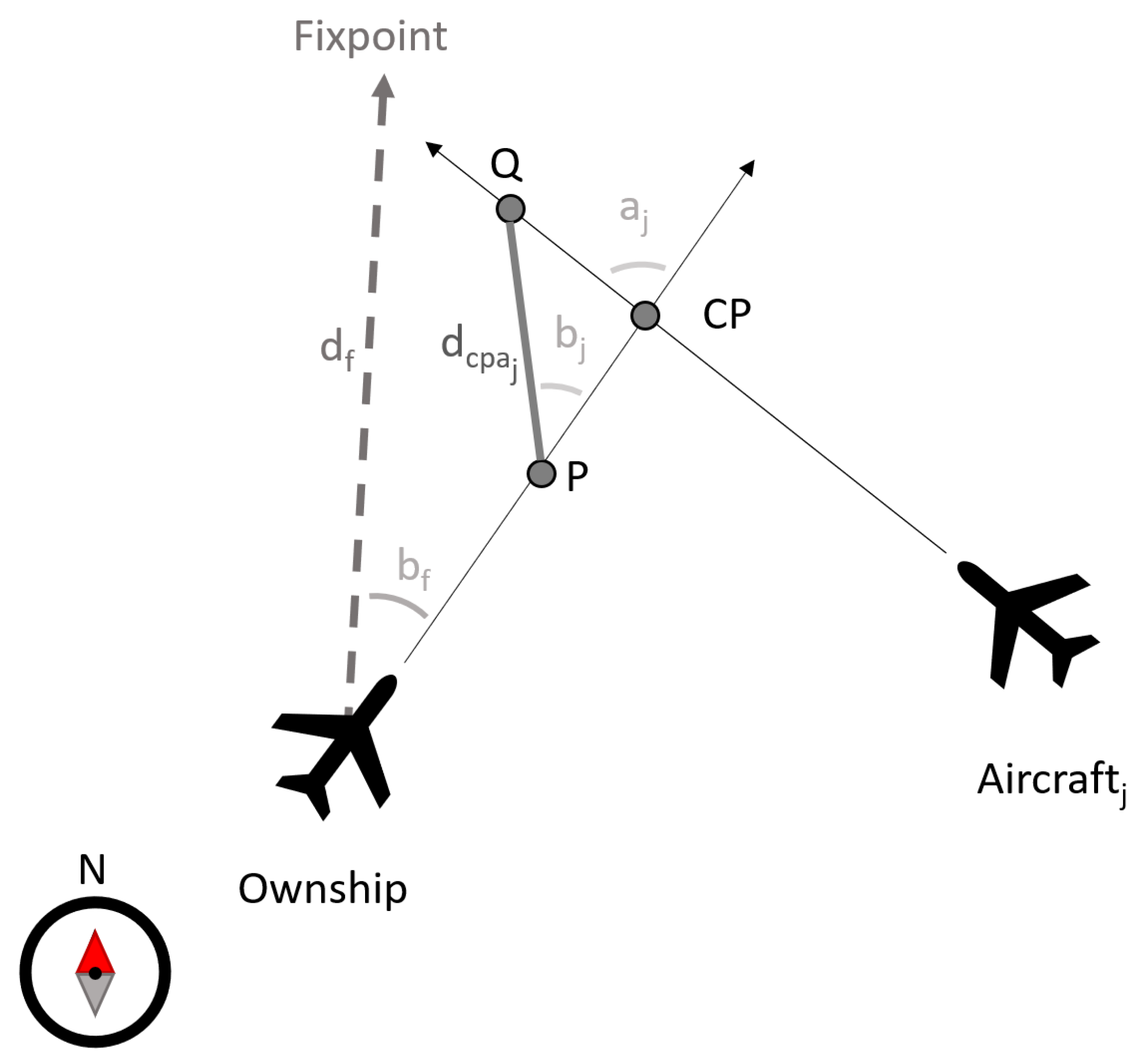
Motivated by the bibliography on CD&R ( [14,15,16,17]), states include features (shown in Figure 3) comprising the relative bearing with regard to a fixpoint (defined subsequently), the distance from that fixpoint, the magnitudes of the aircraft horizontal () and vertical () speed, and the vector , where each includes features of conflicts with neighbor trajectories :
As Figure 3 depicts, and are the horizontal and vertical distances of the ownship from an aircraft j at the CPA, and is the time of the ownship to CPA. is the distance between the ownship and the aircraft j when the first of these is at the crossing point, and is the time until the first of the aircraft is at the crossing point. The intersection angle between the two trajectories is , and is the relative bearing of the ownship with regard to the aircraft j at the CPA.
The is the 2D point at which the boundary of the considered spatiotemporal area SA crosses the line connecting the origin and the destination airports. The fixpoint provides a reference point and allows features to be independent from the airspace and origin–destination pair considered. In doing so, the models trained are generic.
Therefore, the state at a time point t of a flight trajectory (ownship) is of the following form:
Neighbors are sorted in ascending order with regard to and the first values of k are considered. In this work, k is set to 3.
Figure 3.
Features enriching a trajectory point with regard to the aircraft flying a neighbor trajectory . The fixpoint is the 2D point at which the boundary of the spatiotemporal area SA crosses the line connecting the origin and the destination airports.
Figure 3.
Features enriching a trajectory point with regard to the aircraft flying a neighbor trajectory . The fixpoint is the 2D point at which the boundary of the spatiotemporal area SA crosses the line connecting the origin and the destination airports.

The resolution action types considered are as follows:
- -
- : “Speed change resolution action”
- -
- : “Direct to waypoint resolution action”
- -
- : “Radar vectoring resolution action”
These types, according to the ATCO events dataset, are the most frequent ones, providing most of the examples, constituting of the total set of resolution actions in the en route phase of operations.
2.2.3. Learning the ATCO Policy
According to the formulation of the ATCO policy learning problem as a classification task, the goal is to predict the type of the resolution action a prescribed by the ATCOs at any point , where a state with conflicts occurs. Therefore, the aim is to learn a model that maps states to conflict resolution action types a. Formally, the inputs of the models are states, as specified in Section 2.2.2, i.e., , and the outputs are resolution action types. The samples for training the AI/ML models are states labeled with resolution action types.
To learn such models we consider the methods described in the next sections.
Neural Networks
Neural networks [23] (NN) are function approximators able to model complex non-linear functions, and have been applied with great success in many regression and classification problems, as well as for imitating experts’ behavior using behavior cloning [24,25]. Although closely related to our objective, behavior cloning solves a sequential decision problem. In this work, given the historical samples, the classification models predict only the type of the resolution action at a specific conflicting state, without considering subsequent aircraft states. A neural network is trained using gradient descent [26,27,28], tuning its learnable parameters towards optimizing a loss function based on the training examples provided. Different loss functions are applied to different tasks. For our purposes, we apply a common loss function used for classification tasks: the cross-entropy loss. Formally, the following objective is minimized:
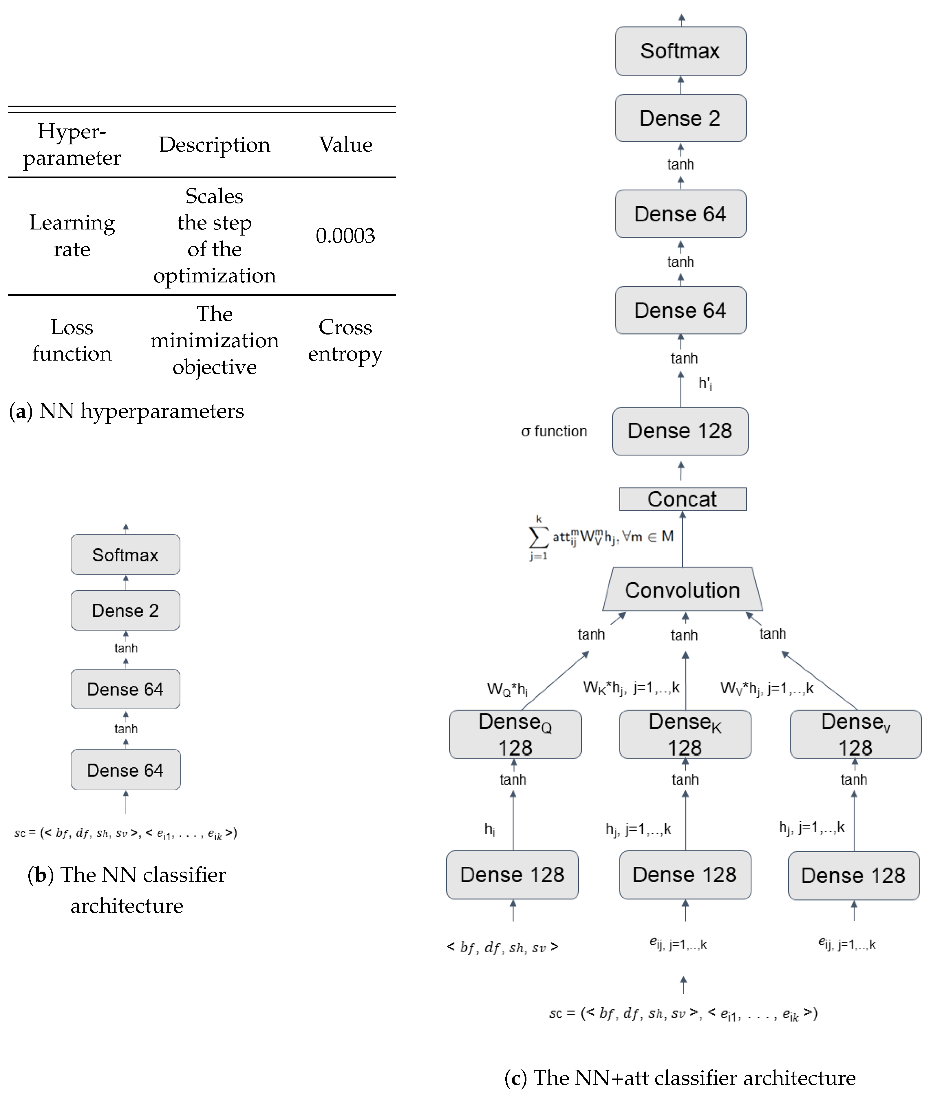
For our purposes, this “simple” NN classifier is augmented with an attention module. The attention module is a convolution layer based on a multi-head dot product attention kernel [29] that models interactions between the ownship and the aircraft executing neighbor trajectories. Specifically, this module introduces vectors of learnable parameters (weights), denoted by , , and , for the projection of features into “queries”, “keys” and “values”, respectively. Dot product attention kernels model interactions by performing dot product multiplication between the query and key values. In the single head attention case, queries, keys, and values are represented with single vectors. In multi-head attention kernels, these vectors are split into a number of vectors, equal to the number of heads. Considering M attention heads, the interaction between the ownship i and one of its neighbors is modeled by the attention head , where m indexes one of the M heads, as follows:
where is a scaling factor and is multiplied with a hidden representation of the ownship’s features and is multiplied with a hidden representation of the ownship neighbours’ features, . The hidden state results from passing the input features from an encoding layer, while results from passing the input features from an encoding layer (a dense layer is used in our case). The M attention heads are combined to the output of the attention module as follows:
where the function is a neural network layer. In our case query, key and value projections and the function are implemented using dense layers of 128 nodes each.
The architecture of the NN, with and without the attention module, and the hyperparameters, are specified in Figure 4.
Specifically, the NN classifier without the attention module comprises two dense hidden layers with 64 nodes, each with tanh activation and L2 (weight decay) regularization [30]. The NN with the attention module passes the output of the attention module to the NN classifier. Figure 4 specifies how the hyperparameters of the networks are set. In order to avoid overfitting, an early stopping mechanism has been used: This is a regularization technique that determines the best amount of epochs to train. Based on the early stopping algorithm described in [31], the model’s training is stopped when the validation error does not improve, and the model is retrained on the training and validation sets for the best number of epochs.
As already pointed out, it is likely that labels (i.e., historical ATCOs resolution action types) of revealed conflicts are noisy, containing trajectory states that are wrongly associated with a resolution action type. Noisy labels can be introduced by (i) the data, as is often the case with real-world data, and by (ii) the conflict detection methodology, which may reveal conflicting situations that do not correspond to the actual ATCO events indicated in the dataset.
According to the survey presented in [32], noise is categorized as instance-independent label noise or instance-dependent label noise. Instance-independent label noise could depend on the label, called label-dependent or asymmetric noise, or could be uniform among all classes, called symmetric noise. Different methods deal with different types of noise in various ways. Some methods change the network architecture to model label noise [33], while others apply forms of regularization to increase models’ robustness, as in [34]. Others propose robust loss functions, as in [35]; make adjustments to the loss function, as in [36]; or select training samples that are noise-free with high probability, as in [37].
To address label noise, we opted for the self-evolution average label (SEAL) method, which is a label refurbishment method presented in [36]. SEAL trains an NN multiple times from scratch. At each SEAL iteration, the model’s output on all samples for each epoch is recorded. Then, for each sample, SEAL computes the average output value over all epochs. This value is considered to be an approximation of the true (not noisy) label and is used as the sample’s label for the next SEAL iteration. In this work, we use five SEAL iterations.
SEAL has the following advantages: It can deal with high rates of noise, does not need a noise-free validation set (in contrast to other methods), uses all training samples (in contrast to sample selection methods), and is robust to instance-dependent noise, which is the most complex form of noise. SEAL is a good fit in our case, as a noise-free subset of the dataset is not available and label noise is likely to be instance-dependent.
Active passive loss functions presented in [35] provide an alternative way to address label noise, and were also tested in this work. An active passive loss function is the weighted sum of an active and a passive loss function. Formally, it has following form, , where are coefficients that balance the two loss functions and L denotes a loss function. A loss function is considered active if it only optimizes the model’s learnable parameters with regard to the correct labels of the sample. It aims to increase the probability the model assigns to the sample’s label. Passive loss functions aim to decrease the probability the model assigns to at least one incorrect label. For the active passive loss function to be robust to label noise, both the active and the passive loss functions should be robust. Functions that are not robust to label noise can be made robust using the following normalization form, , where f denotes the model, x is the model’s input, y represents the corresponding labels and K is the number of different labels.
Random Forest and Gradient Tree Boosting
Decision trees (DT) [38] are models used for classification and regression. In this work, we use decision tree ensembles such as random forest (RF) and gradient tree boosting (GTB) for classification.
Classification trees predict a label by using sequences of rules exploiting the input features. At each step, a rule regarding a specific feature is tested and the answer determines the next rule that will be tested, creating a tree-like structure of rules where rules correspond to tree nodes. Rules are inferred based on the training samples. Algorithms for creating decision trees must determine the rules that best divide the training instances in separate classes. To do so, splits of the training samples produced by potential rules are assessed by a gain function. The gain can be expressed using different criteria, e.g., Gini, and each time the rule with the maximum gain is selected. Samples are split until leaves are pure, containing samples of one class only, or until leaves contain the minimum number of samples. Given a DT, the probability of each class for a given input can be predicted by testing which rules apply to the input features, until reaching a leaf and then calculating the fraction of training samples of the class that correspond to that leaf. The structure of the tree determines how the training instances are divided into different classes and thus determines the effectiveness of the tree in terms of the accuracy of the predictions made. Deep trees with many rules may overfit the training set and fail to generalize properly, whereas small trees may underfit the training set, providing inaccurate predictions. Table 2 reports the hyperparameters used in creating DTs for the RF and GTB ensembles used in this work.
RF [39] is an ensemble of decision trees [38] trained individually on the training set to perform classification or regression tasks. For classification tasks, the output class is decided either by voting, selecting the class predicted by most trees, or by using an average of the predicted probabilities for each class. In this work, the prediction is computed as the average predicted probability for each class of the decision trees.
Trees are trained on a subset of the training set built by drawing samples with replacements. This is known as bootstrapping and it results in reducing the variance at the cost of increasing the bias. A technique used to reduce the variance of a RF model is the random input selection, according to which nodes are split during the construction of the trees using a random subset of the input features. In this work, we use both techniques.
As in many real-world datasets, our dataset is imbalanced, as samples corresponding to a resolution action type, specifically resolution action type , constitute a small proportion of the data. Many classification algorithms cannot accurately predict the minority class of imbalanced datasets as they minimize the overall error and tend to ignore rare samples. In [40], the authors proposed balanced RF and weighted RF to deal with the class imbalance problem. Balanced RF balances the bootstrap samples by randomly selecting the same sample number for all classes. On the other hand, weighted RF assigns weights to each class, giving higher weights to minority classes in order to penalize errors made on samples of the minority classes more heavily.
In this work, we use the RF and weighted RF implementation of scikit-learn and the balanced RF implementation of imbalanced-learn. The hyperparameters have been set as shown in Table 2 and Table 3.
Gradient boosting (GB) [41] is a machine learning method that constructs an additive model consisting of the weighted sum of multiple base models called base learners. More formally, the model learned using the gradient boosting method is of the form , where is the set of input variables, is the base learner functions with learnable parameters , and represents learnable expansion coefficients.
GB starts with a simple initial guess for , usually a constant function, and optimizes the following objective:
with for , where denotes a loss function, the true output value corresponding to , and the number of iterations.
Gradient tree boosting (GTB), which is used in this work, is a specific case of this approach where decision trees [38] are used as the base learners.
3. Results
3.1. Experimental Setting
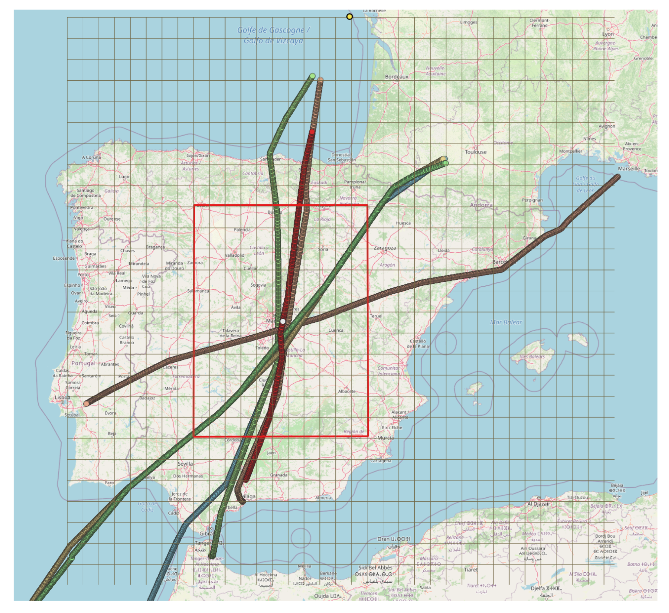
To evaluate the proposed methods, we simulate a flight-centric setting restricted to a rectangular area covering the Iberian Peninsula, as Figure 5 shows. Cells of size degrees (longitude and latitude) segregate this area, creating an index of the positions of trajectories in each cell at each time point. This allows fast access to the trajectories of each cell at each time point, making the identification of neighbor trajectories computationally more efficient. For each point of a focal trajectory, only the neighbor trajectories within a distance threshold of five cells in longitude (approx. 231 km) and latitude (approx. 308 km) are considered. This has as the effect that the area specified by in “follows” the focal trajectory points, i.e., the movement of the ownship.
Figure 5 shows the area considered. The focal trajectory of the ownship is indicated by red (dark gray in grayscale) and other trajectories are the neighbor trajectories in . The ownship position (i.e., the focal trajectory point) at time t is shown in white (middle point). The area defined by with respect to the ownship’s position is depicted by the red rectangle in . The yellow dot in the upper part of the grid is the fixpoint.
To evaluate the effectiveness of the methods in predicting the type of the ATCOs’ resolution actions, we perform five-fold cross-validation, splitting the trajectories into 20% test trajectories and 80% training trajectories. We report on the mean precision, mean recall, and mean f1-score for the resolution action types, , , and , and also the mean Matthews Correlation Coefficient (MCC) across all folds.
Considering the true and predicted classes as two random variables, the MCC is the correlation coefficient between these random variables. For binary classification problems, the MCC is calculated as follows:
where, , , , and , denote the number of true positives, false positives, false negatives, and true negatives, respectively. Therefore, MCC equal to 1 indicates a perfect prediction and 0 a random prediction.
In the multiclass case, MCC is calculated as follows:
with C being the confusion matrix for K classes, the number of times class k truly occurred, the number of times class k was predicted, the total number of samples correctly predicted, and the total number of samples.
3.2. Datasets and Pre-Processing
Following a data-driven approach and exploiting data with flown trajectories, ATCO events must be associated with potential conflicts that have been assessed to exist, either at the point of the ATCO event or in a time window of seconds prior to the ATCO event. However, there are cases where there is an ATCO resolution action for a trajectory but no potential conflicts can be revealed. We filter out these cases. The trajectory point (if any) in the specified time window at which a potential conflict is revealed and is temporally closest to the point of the ATCO event is considered to be the actual resolution action point (mentioned as RATP).
The data include aircraft trajectories flown in 2017 between five different origin–destination pairs: Malaga (LEMG)–Gatwick (EGKK), Malaga (LEMG)–Amsterdam (EHAM), Lisbon (LPPT)–Paris (LFPO), Zurich (LSZH)–Lisbon (LPPT), and Geneva (LSGG)—Lisbon (LPPT). In our study, we consider the en route phase of flights, and thus we filter out resolution actions and trajectory points corresponding to the climb and descent phases of the flights. In addition, we consider only trajectories that have at least one ATCO resolution action of the considered types and an associated RATP. This results in a total of 793 resolution actions associated with 634 trajectories, consisting of 326 “speed change”, 374 “direct to”, and 79 “radar vectoring” actions.
It must be noted that although the available ATCO events dataset covers the Spanish airspace, the proposed method is generic, and can be applied in any airspace.
3.3. Experimental Results
This section presents the experimental results achieved by the AI/ML methods considered, in a comparative way.
Table 5 reports the experimental results achieved by the neural network classifier with an attention mechanism (NN+att) and without attention (NN), in addition to the random forest (RF) and the gradient tree boosting (GTB) algorithms. The columns report the 95% confidence interval of precision, recall, f1-score, and MCC with regard to the resolution action types of ATCOs.
As shown in Table 5, the RF method achieves the best results in terms of the mean MCC and f1-score achieved on the test set, with a mean MCC equal to 0.51 and a mean f1-score equal to 0.73 for resolution action type , 0.76 for resolution type , and for resolution action . The second-best results are provided by the GTB algorithm, achieving a mean MCC value of 0.48 and a mean f1-score 0.69 for resolution action type , 0.74 for resolution type , and 0.48 for resolution action type .
The NN algorithms reported a reduced mean MCC and f1-score compared to RF and GTB. Among the variations tested, the NN+att achieves a mean MCC value of 0.44 and mean f1-score of 0.66, 0.72, and 0.41 for resolution action types , , and , respectively.
The effect of the attention module on the accuracy of the predictions, compared against the variant without attention (NN) is positive: the mean values of the MCC and f1-score increase and the confidence interval becomes narrower. This implies better and more stable performance (reduced standard deviation for independent experiments) among the different folds. This improvement implies that the modeling of interactions between the ownship and its neighbors using a convolution layer results in more useful representations of states.
Considering the capacity of the models, we observe that RF and GTB methods achieve a strong positive correlation between true and predicted , , and resolution action types on the training set, with MCC values ranging from 1 to 0.96, respectively. The f1-scores are also high for RF and GTB, with values in the interval [0.94, 1]. The MCC and f1-scores of NN and NN+att computed for the training set are not so high, due to the early stopping mechanism.
4. Discussion
Given the results reported in Section 3.3, we make the following observations:
- All methods have difficulty in predicting the resolution action type accurately.
- The number of samples might be small, especially for training NN models.
- As discussed in Section 2.2.3, we deal with historical data that do not demonstrate the conflicts occurred; thus, it is likely that the labels (in our case, historical ATCO resolution action types) of revealed conflicts are noisy.
Regarding the first issue, considering that resolution action type is the minority class, we studied the application of different techniques that deal with class imbalance to improve the results of the best method. Specifically, we used sample weights, i.e., RF with class weights, and resampling, i.e., balanced RF (https://imbalanced-learn.org/stable/references/generated/imblearn.ensemble.BalancedRandomForestClassifier.html, accessed on 12 June 2023). We observed that such approaches achieved better results for the minority class but reduced the accuracy of the predictions for the other classes, resulting in a reduced overall accuracy. Specifically, balanced RF achieved a mean MCC score of 0.44 and f1-scores of 0.65, 0.72, and 0.42 for resolution action types , , and , respectively.
Considering the second issue, we augmented the training data by using the trajectory points at which a conflict is detected, in a time window of 250 s before the RATP, as potential conflicting states. These points were labeled with the action type of the corresponding RATP. This is on par with the uncertainty of ATCOs regarding the time to issue a resolution action. This approach did not result in better results, either for the neural network, or for the RF classifiers. This suggests that this type of data augmentation is not beneficial. This could be due either to mislabeled samples inserted into the training set, increasing the label noise, or because this type of augmentation does not effectively cover the feature space.
Noisy labels, as already discussed in Section 2.2.3, could be introduced by (i) the data itself, and by (ii) the conflict detection methodology. To these aspects we should add (iii) the data augmentation process.
As discussed in Section 2.2.3, to address label noise we opted for SEAL. Furthermore, using SEAL on the augmented data improved the accuracy of the predictions. As shown in Table 6, NN with the attention module, SEAL, and data augmentation (NN+att+SEAL+augm) achieved an MCC score of 0.46, which is a +0.02 improvement over NN with the attention module (NN+att). The f1-score for the , , and resolution action types was 0.68, 0.73, and 0.47, respectively. However, this improvement was small and did not manage to outperform RF nor GTB. An important reason for the results achieved by the methods robust to label noise in our case is that such methods are usually validated in noise-free test sets. In our case, the test set contained samples that were as noisy as the training dataset, and, thus, although the method could be robust to label noise, this effect is not evident in a noisy test set.
Finally, we also tested NN+att with the active passive loss functions presented in [35], with data augmentation (NN+att+AP loss+augm). This method did not prove to be robust in instance-dependent noise and did not achieve better results than NN+att. As commented above, noisy samples in the test set could “hide” the effectiveness of the AP loss. As reported in Table 6, the best MCC score achieved was 0.40 and the f1-score for the , , and resolution action types was 0.65, 0.71, and 0.35, respectively. These results were achieved using the normalized cross entropy loss combined with the reverse cross entropy loss and setting the a and b hyperparameters to a = 10 and b = 0.1.
Experiments were ran on an AMD Ryzen 9 3900X 12-Core Processor and NN-based models also utilized a GeForce RTX 2080 Ti Graphics Processing Unit (GPU). Regarding the computational efficiency of the methods, predictions of samples were instant (provided in milliseconds) for all methods. Considering the training time, methods based on RF and GTB completed training in less than one minute. NN-based methods needed more training time, but were still time-efficient, as one experiment completed training in less than an hour. In the case of SEAL, this must be multiplied by the number of SEAL iterations. When comparing NN+att to NN, NN+att is more computationally expensive than NN, as it has more learnable parameters than NN.
5. Conclusions
This work continues our work towards imitating ATCOs, as has been described in [7]. While the aim there was to model ATCOs’ timely reactions in the presence of conflicts between flights, predicting the ATCOs will react, here, our aim is to predict the ATCOs will react, if they do decide to react.
Therefore, this article addresses challenges that result from the inherent imperfections of historical datasets recording trajectories and associated ATCO events, and makes the following contributions regarding the modeling of ATCO policy:
- It specifies a formulation of learning the ATCO policy problem as a classification task;
- It studies enhanced AI/ML methods to learn models of ATCO policy from real-world historical datasets;
- It evaluates the proposed AI/ML methods using real-world data.
The methodology followed in terms of addressing data limitations, and the training of AI/ML models, entails exploiting ATCOs’ expert knowledge regarding (a) the assessment of traffic and potential conflicts the ATCOs might observe, and associating these conflicts with the recorded resolution actions; and (b) how conflicts are resolved by ATCOs, as this is revealed by ATCO events.
The results show that classification methods, such as RF, GTB, and NNs, achieve good accuracy in predicting ATCOs’ actions given specific conflicts, but they have limitations, which are mostly due to the imperfections of the historical datasets exploited.
Indeed, resolution actions predicted by models learned using a data-driven approach, as in this study, will be in the best case as good as the actions included in the historical datasets. If the dataset includes ATCO actions that perform poorly by not effectively solving the detected conflicts, the models will repeat such actions under nearly the same circumstances. Thus, it is important to have datasets containing effective ATCO resolution actions, according to specific objectives. Furthermore, as discussed, knowing the ATCOs’ observations that triggered their resolution actions is essential for the learning process. Historical datasets used in this study do not include these ATCOs’ observations. To address this issue, we projected the aircraft’s position into the future in order to reveal the potential conflicts and the corresponding ATCO’s observations that triggered their resolution action. This was challenging, and introduced noise in the learning process. Deviating from the actual ATCO observations can have a negative effect on the models’ performance.
Other methods such as reinforcement learning algorithms have the ability to explore the state space in a trial-and-error fashion and apply optimization in terms of specific factors, such as conflicts resolved, nautical miles added to the trajectory due to resolution actions, fuel consumption, etc. Such techniques in many cases provide more effective and efficient actions with regard to the optimization objective when compared to human decisions. However, to increase the effectiveness and trustworthiness of automated decision-making agents [6], especially in safety-critical domains such as the ATC, the actions proposed should be similar to the actions taken by human experts.
Future research should involve investigating the combination of supervised learning methods with reinforcement learning techniques, in order to provide resolution actions considering the ATCOs’ preferences, while also optimizing specific objectives with respect to the efficiency of the resolution actions.
Finally, we aim to address the ATCO policy learning problem as a multi-stage imitation learning task, considering the evolution of conflicts. This is rather challenging, and datasets with conflicting situations associated with ATCO events are necessary.
Author Contributions
Conceptualization, G.A.V.; methodology, G.A.V. and A.B.; software, A.B.; validation, A.B.; investigation, G.A.V. and A.B.; data curation, A.B.; writing—original draft preparation, A.B.; writing—review and editing, G.A.V. and A.B.; visualization, A.B.; supervision, G.A.V.; project administration, G.A.V.; funding acquisition, G.A.V. All authors have read and agreed to the published version of the manuscript.
Funding
This research has received funding from the SESAR Joint Undertaking under the European Union’s Horizon 2020 Research and Innovation Programme, grant agreement no. 783287. The opinions expressed herein reflect the authors’ views only. Under no circumstances shall the SESAR Joint Undertaking be responsible for any use that may be made of the information contained herein.
Informed Consent Statement
Not applicable.
Data Availability Statement
Data were provided confidentially by CRIDA (Centro de Referencia de Investigación, Desarrollo e Innovación ATM A.I.E.).
Acknowledgments
The authors express their gratitude to CRIDA (Centro de Referencia de Investigación, Desarrollo e Innovación ATM A.I.E.) for providing the datasets exploited in this study.
Conflicts of Interest
The authors declare no conflict of interest.
References
- NextGen. Available online: https://www.faa.gov/nextgen (accessed on 2 June 2023).
- SESAR Joint Undertaking. Available online: https://www.sesarju.eu/ (accessed on 2 June 2023).
- International Civil Aviation Organization. Annex 11—Air Traffic Services; International Civil Aviation Organization: Montreal, QC, Canada, 2001. [Google Scholar]
- International Civil Aviation Organization. Air Traffic Management-Procedures for Air Navigation Services (Doc 4444); International Civil Aviation Organization: Montreal, QC, Canada, 2007. [Google Scholar]
- Rodríguez, R.; Olbés, A. D2.1 TAPAS Use Cases Description, TAPAS SESAR-ER4-01-2019 Project, Edition 00.01.01. 2020. Available online: https://tapas-atm.eu/wp-content/uploads/2021/06/D2.1_TAPAS-Use-Cases-Description_Ed_00.01.01.pdf (accessed on 2 June 2023).
- Westin, C.; Borst, C.; Kampen, E.J.; Nunes, T.M.M.; Boonsong, S.; Hilburn, B.; Cocchioni, M.; Bonelli, S. Personalized and Transparent AI Support for ATC Conflict Detection and Resolution: An Empirical Study. In Proceedings of the 12th SESAR Innovation Days, Budapest, Hungary, 5–8 December 2022. [Google Scholar]
- Bastas, A.; Vouros, G. Data-driven prediction of Air Traffic Controllers reactions to resolving conflicts. Inf. Sci. 2022, 613, 763–785. [Google Scholar] [CrossRef]
- Ribeiro, M.; Ellerbroek, J.; Hoekstra, J. Review of conflict resolution methods for manned and unmanned aviation. Aerospace 2020, 7, 79. [Google Scholar] [CrossRef]
- Islami, A.; Chaimatanan, S.; Delahaye, D. Large-Scale 4D Trajectory Planning. In Air Traffic Management and Systems II: Selected Papers of the 4th ENRI International Workshop, 2015; Institute, Electronic Navigation Research, Ed.; Springer: Tokyo, Japan, 2017; pp. 27–47. [Google Scholar] [CrossRef]
- Dougui, N.; Delahaye, D.; Puechmorel, S.; Mongeau, M. A light-propagation model for aircraft trajectory planning. J. Glob. Optim. 2013, 56, 873–895. [Google Scholar] [CrossRef] [Green Version]
- Durand, N.; Gotteland, J.B. Genetic Algorithms Applied to Air Traffic Management. In Metaheuristics for Hard Optimization: Simulated Annealing, Tabu Search, Evolutionary and Genetic Algorithms, Ant Colonies,… Methods and Case Studies; Springer: Berlin/Heidelberg, Germany, 2006; pp. 277–306. [Google Scholar] [CrossRef]
- Srivatsa, M.; Ganti, R.; Chu, L.; Christiansson, M.; Nilsson, J.; Rydell, S.; Josefsson, B. Towards AI-based Air Traffic Control. In Proceedings of the ATM Seminar 2021, Virtual Event, 20–23 September 2021. [Google Scholar]
- Ayhan, S.; Costas, P.; Samet, H. Prescriptive analytics system for long-range aircraft conflict detection and resolution. In Proceedings of the 26th ACM SIGSPATIAL, Seattle, WA, USA, 6–9 November 2018; pp. 239–248. [Google Scholar] [CrossRef]
- Pham, D.T.; Tran, N.P.; Goh, S.K.; Alam, S.; Duong, V. Reinforcement learning for two-aircraft conflict resolution in the presence of uncertainty. In Proceedings of the 2019 IEEE-RIVF, Danang, Vietnam, 20–22 March 2019; pp. 1–6. [Google Scholar] [CrossRef]
- Pham, D.T.; Tran, N.P.; Alam, S.; Duong, V.; Delahaye, D. A machine learning approach for conflict resolution in dense traffic scenarios with uncertainties. In Proceedings of the ATM Seminar 2019, Vienna, Austria, 17–21 June 2019. [Google Scholar]
- Dalmau, R.; Allard, E. Air Traffic Control using message passing neural networks and multi-agent reinforcement learning. In Proceedings of the 10th SESAR Innovation Days, Virtual Event, 7–10 December 2020; pp. 7–10. [Google Scholar]
- Ghosh, S.; Laguna, S.; Lim, S.H.; Wynter, L.; Poonawala, H. A deep ensemble multi-agent reinforcement learning approach for air traffic control. arXiv 2020, arXiv:2004.01387. [Google Scholar] [CrossRef]
- Isufaj, R.; Sebastia, D.A.; Piera, M.A. Towards Conflict Resolution with Deep Multi-Agent Reinforcement Learning. In Proceedings of the ATM Seminar 2021, Virtual Event, 20–23 September 2021. [Google Scholar]
- Calvo-Fernández, E.; Perez-Sanz, L.; Cordero-García, J.M.; Arnaldo-Valdés, R.M. Conflict-free trajectory planning based on a data-driven conflict-resolution model. J. Guid. Control. Dyn. 2017, 40, 615–627. [Google Scholar] [CrossRef]
- Tran, N.P.; Pham, D.T.; Goh, S.K.; Alam, S.; Duong, V. An Intelligent Interactive Conflict Solver Incorporating Air Traffic Controllers’ Preferences Using Reinforcement Learning. In Proceedings of the IEEE Integrated Communications, Navigation and Surveillance Conference, Herndon, VA, USA, 9–11 April 2019; pp. 1–8. [Google Scholar] [CrossRef]
- van Rooijen, S.J.; Ellerbroek, J.; Borst, C.; van Kampen, E. Toward Individual-Sensitive Automation for Air Traffic Control Using Convolutional Neural Networks. J. Air Transp. 2020, 28, 105–113. [Google Scholar] [CrossRef]
- Erzberger, H. Automated conflict resolution for air traffic control. In Proceedings of the 25th International Congress of the Aeronautical Sciences, Hamburg, Germany, 3–8 September 2006; National Aeronautics and Space Administration, Ames Research Center: Mountain View, CA, USA, 2006. [Google Scholar]
- Bishop, C.M. Neural networks and their applications. Rev. Sci. Instrum. 1994, 65, 1803–1832. [Google Scholar] [CrossRef] [Green Version]
- Codevilla, F.; Santana, E.; López, A.M.; Gaidon, A. Exploring the limitations of behavior cloning for autonomous driving. In Proceedings of the IEEE/CVF International Conference on Computer Vision, Seoul, Republic of Korea, 27 October–2 November 2019; pp. 9329–9338. [Google Scholar]
- Pomerleau, D.A. Alvinn: An autonomous land vehicle in a neural network. Adv. Neural Inf. Process. Syst. 1988, 1, 305–313. [Google Scholar]
- Amari, S.i. Backpropagation and stochastic gradient descent method. Neurocomputing 1993, 5, 185–196. [Google Scholar] [CrossRef]
- Ruder, S. An overview of gradient descent optimization algorithms. arXiv 2016, arXiv:1609.04747. [Google Scholar]
- Bishop, C.M. Pattern Recognition and Machine Learning (Information Science and Statistics); Springer: Berlin/Heidelberg, Germany, 2006; Volume 4. [Google Scholar] [CrossRef] [Green Version]
- Vaswani, A.; Shazeer, N.; Parmar, N.; Uszkoreit, J.; Jones, L.; Gomez, A.N.; Kaiser, Ł.; Polosukhin, I. Attention is all you need. Adv. Neural Inf. Process. Syst. 2017, 30, 5998–6008. [Google Scholar]
- Bishop, C.M. Regularization and Complexity Control in Feed-Forward Networks; Aston University (General): Birmingham, UK, 1995. [Google Scholar]
- Goodfellow, I.; Bengio, Y.; Courville, A. Deep Learning; MIT Press: Cambridge, MA, USA, 2016; Available online: http://www.deeplearningbook.org (accessed on 12 June 2023).
- Song, H.; Kim, M.; Park, D.; Shin, Y.; Lee, J.G. Learning from noisy labels with deep neural networks: A survey. IEEE Trans. Neural Netw. Learn. Syst. 2022, 1–19. [Google Scholar] [CrossRef] [PubMed]
- Han, B.; Yao, J.; Niu, G.; Zhou, M.; Tsang, I.; Zhang, Y.; Sugiyama, M. Masking: A new perspective of noisy supervision. Adv. Neural Inf. Process. Syst. 2018, 31, 5836–5846. [Google Scholar]
- Xia, X.; Liu, T.; Han, B.; Gong, C.; Wang, N.; Ge, Z.; Chang, Y. Robust early learning: Hindering the memorization of noisy labels. In Proceedings of the International Conference on Learning Representations, Vienna, Austria, 3–7 May 2021. [Google Scholar]
- Ma, X.; Huang, H.; Wang, Y.; Romano, S.; Erfani, S.; Bailey, J. Normalized loss functions for deep learning with noisy labels. In Proceedings of the International Conference on Machine Learning, PMLR, Virtual Event, 12–18 July 2020; pp. 6543–6553. [Google Scholar]
- Chen, P.; Ye, J.; Chen, G.; Zhao, J.; Heng, P.A. Beyond class-conditional assumption: A primary attempt to combat instance-dependent label noise. In Proceedings of the AAAI Conference on Artificial Intelligence, Virtual Event, 2–9 February 2021; Volume 35, pp. 11442–11450. [Google Scholar]
- Nguyen, D.T.; Mummadi, C.K.; Ngo, T.P.N.; Nguyen, T.H.P.; Beggel, L.; Brox, T. Self: Learning to filter noisy labels with self-ensembling. arXiv 2019, arXiv:1910.01842. [Google Scholar]
- Kotsiantis, S.B. Decision trees: A recent overview. Artif. Intell. Rev. 2013, 39, 261–283. [Google Scholar] [CrossRef]
- Breiman, L. Random forests. Mach. Learn. 2001, 45, 5–32. [Google Scholar] [CrossRef] [Green Version]
- Chen, C.; Liaw, A.; Breiman, L. Using Random Forest to Learn Imbalanced Data; University of California: Berkeley, CA, USA, 2004; Volume 110, p. 24. [Google Scholar]
- Friedman, J.H. Stochastic gradient boosting. Comput. Stat. Data Anal. 2002, 38, 367–378. [Google Scholar] [CrossRef]
Figure 1.
Methodology stages for learning the ATCO policy.

Figure 2.
Trajectory points (blue points) and an associated air traffic controller (ATCO) event. Table columns correspond to the callsign, the departure (apt_from), and the destination airports (apt_to), the resolution action type (mwm_code), the unix epoch timestamp (the number of seconds that have elapsed since 1 January 1970, midnight UTC (Universal Time Coordinated)/GMT (Greenwich Mean Time)) (time_annotation) and the sector in which the resolution action was taken (sector). The red point shows the aircraft’s trajectory point (with the timestamp) associated with the ATCO event.

Figure 4.
The neural network (NN) and neural network with attention (NN+att) hyperparameters (a), the NN classifier without attention (b), and the NN classifier with attention (c). , , and denote the query, key, and value projections, respectively.
Figure 4.
The neural network (NN) and neural network with attention (NN+att) hyperparameters (a), the NN classifier without attention (b), and the NN classifier with attention (c). , , and denote the query, key, and value projections, respectively.

Figure 5.
The area and the area defined by (red rectangular area) with regard to the ownship’s position (white dot).
Figure 5.
The area and the area defined by (red rectangular area) with regard to the ownship’s position (white dot).


Table 1.
Problem-specific parameters.
| Parameter | Description | Value |
|---|---|---|
| The crossing time threshold. | 20 min | |
| Time to closest point of approach (CPA) threshold | 20 min | |
| The horizontal distance threshold between aircraft at the CPA. | 15 NM | |
| The vertical distance threshold. | 1000 ft below flight level (FL) 420, 2000 ft else |
Table 2.
Hyperparameters of the decision trees used for the random forest (RF) and gradient tree boosting (GTB) algorithms. Descriptions are from scikit-learn.
Table 2.
Hyperparameters of the decision trees used for the random forest (RF) and gradient tree boosting (GTB) algorithms. Descriptions are from scikit-learn.
| Hyperparameter | Description | RF Value | GTB Value |
|---|---|---|---|
| criterion | The function to measure the quality of a split. | gini | friedman mse |
| max_depth | The maximum depth of the tree. If None, then nodes are expanded until all leaves are pure (containing one class only) or until all leaves contain less than min_samples_split samples. | None | 3 |
| min_samples_split | The minimum number of samples required to split an internal node. | 2 | 2 |
| min_samples_leaf | The minimum number of samples required to be at a leaf node. | 1 | 2 |
| min_weight_fraction_leaf | The minimum weighted fraction of the sum total of weights (of all the input samples) required to be at a leaf node. | 0 | 0 |
| max_features | The number of features to consider when looking for the best split. If “sqrt”, then max_features is equal to the square root of the total number of features. If None, then max_features is equal to the number of total features. | sqrt | None |
| max_leaf_nodes | Trees grown with max_leaf_nodes in best-first fashion. Best nodes are defined as a relative reduction in impurity. If None then unlimited number of leaf nodes. | None | None |
| min_impurity_decrease | A node will be split if this split induces a decrease in the impurity greater than or equal to this value. | 0 | 0 |
| ccp_alpha | Complexity parameter used for minimal cost-complexity pruning. The subtree with the largest cost complexity that is smaller than ccp_alpha will be chosen. When 0, no pruning is performed. | 0 | 0 |
Table 3.
Hyperparameters used for the random forest (RF) algorithm. Descriptions are from scikit-learn.
Table 3.
Hyperparameters used for the random forest (RF) algorithm. Descriptions are from scikit-learn.
| Hyperparameter | Description | Value |
|---|---|---|
| n_estimators | The number of trees in the ensemble. | 100 |
| bootstrap | Whether bootstrap samples are used when building trees. If False, the whole dataset is used to build each tree. | True |
| oob_score | Whether to use out-of-bag samples (samples that have not been used when bootstrapping) to estimate the generalization score. | False |
| class_weight | Weights associated with classes. If None, all classes are supposed to have weight one. | None |
| max_samples | If bootstrap is True, draw a number of samples from the training set to train each base estimator. If None, then draw a number of samples equal to the size of the training set. | None |
| random_state | Controls both the randomness of the bootstrapping of the samples used when building trees (if bootstrap=True) and the sampling of the features to consider when looking for the best split at each node (if max_features < total number of features). | None |
Table 4.
Hyperparameters of the gradient tree boosting algorithm. Descriptions are from scikit-learn.
Table 4.
Hyperparameters of the gradient tree boosting algorithm. Descriptions are from scikit-learn.
| Hyperparameter | Description | Value |
|---|---|---|
| n_estimators | The number of trees in the ensemble. | 100 |
| loss | The loss function to be optimized. | log_loss |
| learning rate | Shrinks the contribution of each tree. | 0.1 |
| subsample | The fraction of samples to be used for fitting the individual base learners. | 1 |
| init | An estimator that is used to compute the initial predictions. If None, the initial estimator predicts the classes’ priors. | None |
| validation_fraction | The proportion of training data to set aside as the validation set for early stopping. Only used if n_iter_no_change is set to an integer. | Not used |
| n_iter_no_change | Used to decide if early stopping will be used to terminate training when the validation score does not improve. If None, early stopping is disabled. | None |
| random_state | Controls the random seed given to each Tree estimator at each boosting iteration. In addition, it controls the random permutation of the features at each split. | None |
| tol | Tolerance for early stopping. When the loss is not improving by at least tol for n_iter_no_change iterations (if set to a number), the training stops. | 1 × 10⁻⁴ |
Table 5.
Experimental results achieved by the neural network classifier with an attention mechanism (NN+att) and without attention (NN), in addition to the random forest (RF) and the gradient tree boosting (GTB) algorithms. Columns report the 95% confidence interval of precision, recall, f1-score, and MCC with regard to the resolution action types of ATCOs.
| Method | Dataset | Precision | Recall | f1-Score | MCC | ||||||
|---|---|---|---|---|---|---|---|---|---|---|---|
| NN | train | ||||||||||
| test | |||||||||||
| NN+att | train | ||||||||||
| test | |||||||||||
| RF | train | ||||||||||
| test | |||||||||||
| GTB | train | ||||||||||
| test | |||||||||||
Table 6.
Experimental results achieved by balanced random forest (balanced RF), neural network with attention SEAL and data augmentation (NN+att+SEAL+augm), and neural network with attention active passive loss and data augmentation (NN+att+AP loss+augm). Columns report the 95% confidence interval of precision, recall, f1-score, and MCC with regard to the resolution action types of ATCOs.
| Method | Dataset | Precision | Recall | f1-Score | MCC | ||||||
|---|---|---|---|---|---|---|---|---|---|---|---|
| Balanced RF | train | ||||||||||
| test | |||||||||||
| NN+att+AP loss+augm | train | ||||||||||
| test | |||||||||||
| NN+att+SEAL+augm | train | ||||||||||
| test | |||||||||||
Disclaimer/Publisher’s Note: The statements, opinions and data contained in all publications are solely those of the individual author(s) and contributor(s) and not of MDPI and/or the editor(s). MDPI and/or the editor(s) disclaim responsibility for any injury to people or property resulting from any ideas, methods, instructions or products referred to in the content. |
© 2023 by the authors. Licensee MDPI, Basel, Switzerland. This article is an open access article distributed under the terms and conditions of the Creative Commons Attribution (CC BY) license (https://creativecommons.org/licenses/by/4.0/).
Share and Cite
MDPI and ACS Style
Bastas, A.; Vouros, G.A. Data-Driven Modeling of Air Traffic Controllers’ Policy to Resolve Conflicts. Aerospace 2023, 10, 557. https://doi.org/10.3390/aerospace10060557
AMA Style
Bastas A, Vouros GA. Data-Driven Modeling of Air Traffic Controllers’ Policy to Resolve Conflicts. Aerospace. 2023; 10(6):557. https://doi.org/10.3390/aerospace10060557
Chicago/Turabian StyleBastas, Alevizos, and George A. Vouros. 2023. "Data-Driven Modeling of Air Traffic Controllers’ Policy to Resolve Conflicts" Aerospace 10, no. 6: 557. https://doi.org/10.3390/aerospace10060557
Note that from the first issue of 2016, this journal uses article numbers instead of page numbers. See further details here.