
Adjoint and Direct Characteristic Equations for Two-Dimensional Compressible Euler Flows

1
Département Aérodynamique, Aéroélasticité et Acoustique (DAAA), ONERA, Université Paris Saclay, 29 Avenue de la Division Leclerc, Châtillon, 92322 Paris, France
2
Département Aérodynamique, Aéroélasticité et Acoustique (DAAA), ONERA, Université Paris Saclay, 8 Rue des Vertugadins, 92190 Meudon, France
*
Author to whom correspondence should be addressed.
Aerospace 2023, 10(9), 797; https://doi.org/10.3390/aerospace10090797
Submission received: 20 July 2023
/
Revised: 8 September 2023
/
Accepted: 10 September 2023
/
Published: 12 September 2023
(This article belongs to the Special Issue Adjoint Method for Aerodynamic Design and Other Applications in CFD)
Abstract
:The method of characteristics is a classical method for gaining understanding in the solution of a partial differential equation. It has recently been applied to the adjoint equations of the 2D steady-state Euler equations and the first goal of this paper is to present a linear algebra analysis that greatly simplifies the discussion of the number of independent characteristic equations satisfied along a family of characteristic curves. This method may be applied for both the direct and the adjoint problem. Our second goal is to directly derive in conservative variables the characteristic equations of 2D compressible inviscid flows. Finally, the theoretical results are assessed for a nozzle flow with a classical scheme and its dual consistent discrete adjoint.
1. Introduction
The method of characteristics is a well-known method for studying partial differential equations (PDEs). It aims to exhibit specific hypersurfaces in the input domain where the solution of the PDE of interest satisfies an ordinary differential equation (ODE). When applied to 2D steady-state inviscid compressible flows, it is known to provide a full resolution of a supersonic area based only on the knowledge of the inflow (whereas it provides partial information for a subsonic flow) [1,2,3,4]. Both a theoretical understanding and practical calculations of a variety of flows (in nozzles, along steps, along curved walls) are enabled by this technique.
In addition, discrete and continuous adjoint are now well-established methods for shape optimization [5,6,7,8,9] and goal-oriented mesh adaptation [10,11,12]. Because of these important applications, regular efforts have been devoted to the fast and safe writing of adjoint modules [13,14,15,16] and to the efficient solving of the adjoint equations [17,18]. Adjoint methods are also useful for flow control [19,20], meta-modeling [21,22], receptivity–sensitivity–stability analyses [23,24], and data assimilation [25,26].
Moving from direct to adjoint Euler equations, the classical flux Jacobians are replaced in the PDE by the opposite of their transpose. This allows the simple adaptation in 2D and 3D of the characteristic equations in the specific sense of the quasi-one-dimensional scalar propagation equations satisfied in the direction normal to a boundary [27]. From the earliest works on the continuous adjoint method, it has been proved that for the adjoint problem (a) information travels along characteristics in the opposite direction to the flow, and (b) the right eigenvectors of the local Jacobian replace the left eigenvectors in the equation definition [5,28,29]. In addition, in a recent paper, the characteristic equations (CEs), in the sense of nonlinear ODEs satisfied along curves to be defined, have been derived for the adjoint 2D steady-state Euler equations [30].
The classical direct characteristic equations (DCEs) for 2D inviscid compressible flows and the recently presented corresponding adjoint characteristic equations (ACEs) appear to be linked; in particular, the characteristic curves are the same for both problems [30]. The analogies between ACEs and DCEs are further studied in Section 2, where several properties of a generic system of equations embedding ACEs and DCEs are demonstrated. In particular, this formal linear algebra approach greatly simplifies the determination of the number of independent CEs satisfied along two families of characteristic curves.
Whereas the ACEs need to be derived from the complete 8 × 8 linear system for the Cauchy problem, the DCEs have been derived with various mechanical assumptions and also various sets of variables [3,4,31,32]. For the sake of a full understanding, the direct characteristic problem is solved in conservative variables from the complete Cauchy problem and the resulting differential forms are discussed in Section 3.
2. Common Properties of Linear Systems for the Cauchy Direct and Adjoint Problems
2.1. Notation, Steady-State Euler Equations
We denote by the conservative variables, with being the density, the components of the velocity , e the internal energy, and E the total energy. A thermally and calorically perfect gas law is considered. The static pressure p, total enthalpy H, and entropy S are
with a constant and a constant heat capacity at constant volume . A subscript i is used to denote the classical stagnation quantities . The steady-state Euler equations read
with and the fluxes along x and y,
or equivalently,
The Euler flux Jacobian matrices in the x- and y-directions, A and B, are equal to
with . The columns of the Jacobians are denoted by to and to such that , . Finally, the discrete adjoint vector of the functional output of interest is denoted as .
2.2. Generic Cauchy Problem Embedding ACE and DCE Base Equations
Given a and b, two neighboring points in the fluid domain, we denote by and then and The increment in the conservative variables between the two points is denoted as and the increment in the adjoint vector components as . The Cauchy problem for the conservative variables aims at calculating their derivatives at point a with first order in space, and the singularities of this problem are at the core of the search of the CEs. The corresponding 8 × 8 linear system associates first-order Taylor expansions and the 2D steady-state Euler equations. The complete system is
The corresponding linear system for the derivatives of the adjoint vector reads
where and are the opposite and transposed Jacobians of the Euler fluxes. The straightforward counterpart for the derivatives of the discrete flow field W, appears in Equation (4). Several results regarding the minors of the matrices in (4) and (5), and also the number of independent CEs when (,) makes the 8 × 8 matrices singular, may be demonstrated by considering a generic matrix and a generic linear system
where stands either for or for . The corresponding generic notation for or W is . The columns of and are denoted as and , respectively. We stress that the bold characters are, therefore, associated with the generic problem and not with a higher tensor order.
2.3. Coefficients of ACE and DCE as Determinants
It has already been observed that the direct and adjoint problems share the same determinant, computed using linear combinations of columns, as
with
using the known eigenvalues of the Euler flux Jacobian in an arbitrary direction [30]. If , the Cauchy problem is well posed, and the solution is expressed using the minors of . These minors are denoted as and with indices referring to the considered variable and the direction of differentiation. For example, is
Conversely, the generic Cauchy problem is ill posed if and only if , that is, along the S, C, and C curves:
In such cases, the boundedness of along the characteristic curves and their expression outside these curves yields the CE. Typically, Equation (7), that is valid outside the characteristic curves, yields the following CE:
along the characteristic curves. Of course, seven other CEs are derived from the boundedness of … and we need to determine a minimal set of independent CEs for each type of characteristic curve.
To that end, the and minors are expressed as determinants of matrices. From Equations (6) and (7),
is the basic formula for . In all 32 corresponding expressions, the terms of the first three lines are eliminated by linear combinations of columns and the determinants are then expanded along these lines. We assume that using and will further consider this hypothesis in the following. For the sake of brevity, we shall not discuss the simple specific case where .
The minors arising in the CE derived from the existence of then read
and the corresponding expressions for are
It is clear that
In addition, expanding along the first line of the matrix results in
so that along a characteristic curve . Corresponding equations are found for the other variables : if whatever the value of and if If the minors are not all null, this proves that the four CEs derived from the boundedness of and their counterparts derived from the boundedness of are proportional, so that only one set has to be studied. At this point, the case of the S curves and the one of the C and C curves shall be discussed separately.
2.4. Number of independent CEs along the C and C
The abstract linear algebra point of view allows us to calculate the number of independent CEs in the specific case of the C and C curves. For , is easily found to be equivalent to
When the value t is the one corresponding to a C or a C, for both the adjoint and the direct problem, the rank of is known to be three from the eigenanalysis of the Euler equations’ flux Jacobians. Using classical theorems for the ranks of block diagonal matrices and the ranks of equivalent matrices, the rank of is easily proved to be seven, one less than its size. In this case, the adjugate matrix is known to have rank one. This means that all CEs (whose coefficients appear in the rows of the adjugate matrix) are proportional and reduced to only one independent equation. This result is very valuable as the corresponding explicit calculations from the algebraic expressions of the minors are very tedious. It has been used in Section 3.4.
2.5. Nullity of All Minors along the S Curves
The determinant involved in the expression of is
Along a streamtrace and is a matrix of rank two. As all its minors of rank three are null, the determinant (13), calculated by expansion along the first column, appears to be zero. To obtain the same property for , , and a straightforward rewriting is needed. For example, the determinant in reads
Under this latter form, it is clearly null when the rank of is two. Using the exact same arguments, it is possible to prove that all and are null when .
In addition, we may change our point of view and consider (13) as a function of t for fixed W. This function is obviously a polynomial of maximum degree three and is one of its roots. We, therefore, expect to be a factor of all , algebraic expressions. The explicit expressions of the coefficients for the ACEs (see [30]) and DCEs (see Appendix A) confirm this property.
Along the S curves, is found to have rank six thanks to the technique used in the previous subsection. As already stated, all and are zero and the adjugate matrix of is the null matrix. The derivation of the explicit CE along the trajectories then involves the multiplicity two of and simplified , coefficients derived by removing in the expressions of the corresponding , . The proportionality of the explicit CEs derived from the boundedness of and is verified but is more easily presented based on the actual formulas of the CEs—see Section 3 for the DCEs and in Section 2 of [30] for the ACEs.
3. Derivation of Characteristic Equations for 2D Inviscid Compressible Flows Using Conservative Variables
3.1. Flow Properties, Sets of Variables, Resulting Equations for the Usual Derivation of the Characteristic Equations
The classical derivations of the DCEs use a set of Taylor expansions and mechanical equations for the variations of a set of primitive variables. These resulting equations are linear in the unknown derivatives of the primitive variables with nonlinear functions of the state variables as coefficients. The variations are generally expressed in an orthonormal frame of reference . This frame is defined by its angle with respect to the one induced by the local flow motion that we denote as (,), with the angle of with respect to the x-axis. This approach leads to simpler expressions for the mechanical equations. Some orientations of the vector make the set of equations ill posed: for all flow regimes and if the flow is locally supersonic. The curves where at each point the tangent vector has one of these specific orientations with respect to the velocity are, respectively, the aforementioned streamtraces S, C (for ) and C (for ). Along these curves, equations with only derivatives are satisfied. These ODEs are the classical DCEs.
For a 2D flow of an ideal gas (Section 2.1), without any assumptions of constant stagnation enthalpy, or constant entropy or null vorticity, (a) the stagnation enthalpy and entropy are found to be constant along streamtraces; and (b) one DCE is found along the CC [3]. This DCE, expressed in terms of variations in , , S, and H, reads
where the Crocco equation can be used to rewrite the last term. If H is constant over the whole fluid domain, the DCE also reads
If S is also constant, the flow is irrotational according to Crocco’s theorem and the DCE reads
This equation can be integrated using the Prandtl–Meyer function,
and the final algebraic equations resulting from the integration of (16) are
Other sets of primitive variables may be used to derive (14) and the resulting simplified equations [4,31]. Also possible is the demonstration of these equations in a mapping of the plane rather than in the aforementioned frame of reference [31].
In case the flow is assumed to be irrotational from the beginning, a very fast demonstration is possible involving the velocity potential—see [32] or [2,34,35]. The governing nonlinear equation for a two-dimensional potential flow is:
and of course
This results in a simple linear system for , , and (that is equal to for the potential flow) from which (16) and (17) are easily derived.
3.2. Derivation of the Characteristic Equations in Conservative Variables
The Cauchy problem aims at computing the derivatives and from the values of W at two neighboring points a and b. The relevant linear system has been posed in Section 2.2 in Equation (4). Its determinant is easily calculated as
Of course, and the problem is ill posed along the S, C, and C curves, as recalled in Section 2.3. The fact that the Cauchy problem is ill posed along these specific curves, whereas and are actually defined and bounded, implies that not only the denominator in the Cramer formula applied to (4) is equal to zero, but also the eight numerators corresponding to the unknowns , , , , , , and must be equal to zero. This is precisely the principle of the method of characteristics that allows ODEs to be derived along the characteristic curves.
The principle of the calculation of the ODE satisfied along the S, C, and C curves is recalled for variable , the boundedness of which requires that
The determinant is expanded along the first column with the notation of the next equation:
In this equation, for example
Finally,
At this step, there is no assumption on the value of t with respect to the velocity vector . The other terms of the differential form are equal to
The characteristic Equation (21) can, thus, be rewritten as
If and , this equation may be further simplified:
Of course, along the S curves, is null and Equation (28) seems to be only valid for the C and C curves. Actually, as has a multiplicity of two in the determinant D, (28) is also needed for the existence of along the S curves (see Section 3.3).
For the other seven partial derivatives, the expressions of the coefficients of the CEs are presented in Appendix A. In addition, it has been proved in Section 2 that, being one of the four conservative variables, the equations for the boundedness of and along the characteristics are proportional by a factor of . Therefore, only the counterparts of Equation (28) for the existence of , , and are presented hereafter:
3.3. Ordinary Differential Equations along the Streamtraces S
Along the trajectories, is a zero of the denominator of Cramer’s formulas with a multiplicity of two. The term appears to be a factor of all and the expressions obtained by removing this term from are denoted by . Obviously wherever the Cauchy problem is well defined
If the point a is fixed and the neighboring point b is moved closer and closer to S, and the boundedness of requires the numerator of (32) to be equal to zero:
The expressions for the coefficients are much simpler than those of the K coefficients thanks to the nullity of . It can be verified by hand or by formal calculation that the CEs expressing the boundedness of and their counterparts for are proportional by a factor of . It is also possible to check that and then use the continuity of the coefficients as functions of and the validity of outside the variety . We denote as G; the fully simplified differential forms then read
where Equation (35) is obtained twice, from the existence of the derivatives of both momentum components. The rank of the matrix was first calculated with the Maple software 2020.0 (Supplementary Materials) and, as expected, is two. It can also be verified by hand calculation that (34) minus (35) is exactly Equation (36) and then, finally, that the and columns in {(34),(35)} are not linked.
Along the streamtraces, the derivative of the total enthalpy, H, and the entropy, S, are expected to be null [27,32]. Before verifying that these properties are ensured by the CE found just before, the differential of times and the differential of H times are calculated:
Equation (34) is exactly the same as . This yields and obviously the derived CEs contain the property of constant entropy along the streamtraces. In addition, (34) plus (36) yields, after simplification by a common factor, . Finally, adding this equation to times Equation (34), precisely yields , so that the second expected property for Euler flows along the trajectories is contained in the derived CEs. Of course, the conservation of the stagnation enthalpy and the entropy along the trajectories of a steady-state inviscid flow is also verified in 3D [27,32].
3.4. Ordinary Differential Equations along the CC
The proportionality of all eight differential forms along the C and C has been proved in Section 2.4 and Equation (28) may be retained as the relevant DCE. The factor of is quite complex in (28) but it admits a simpler form derived from the degree two equations satisfied by and : these curve slopes are defined as
or alternatively by their explicit expressions [30]:
They are the two roots of the following degree two equation [30]
which allows the expression of (28) to be simplified along a C or a C. The final DCE reads
with for a C and by for a C.
It has been first checked that this C(resp. C) differential form is linked with (resp. ) consistently with Equation (14). It is proved in Appendix B that these CEs, expressed with different variables, are the same.
4. Assessment of the Direct and Adjoint Characteristic Equations for a Nozzle Flow
4.1. Supersonic Nozzle Configuration
The test case for the assessment of the DCEs and ACEs is a supersonic nozzle designed for an aircraft flying at Mach 1.6. The geometry was defined in the framework of the SENECA EU project [36]. The nozzle is a classical convergent–divergent duct. At the subsonic injection plane, the stagnation conditions are fixed as well as the direction of the velocity (aligned with the x-axis). The ratios of the far-field flow total pressure (resp. temperature) to the total pressure (resp. total temperature) at the inlet are and . As an inviscid flow is calculated, these two conditions and the far-field Mach number fully define the flow. Figure 1 shows a structural diagram of the case object and the fluid domain.
The original geometry was designed for a circular axisymmetric engine and the nozzle contour in the symmetry plane was simply extracted to define the 2D geometry. Consequently, the mass flow rates are different. Due the different laws of areas along the x-coordinate (the inlet and main flow direction), the flows are also different along the midline of the nozzle. Nevertheless, the Mach number distribution along this line is similar, with at the throat and at the exit.
The functional output of interest is the thrust ,
where is the internal wall of the nozzle, the injection section—see Figure 2—, and the x-component of the surface vector (oriented towards the outside of the fluid domain).
4.2. Flow Calculation, Flow Analysis
A structured eight-block mesh with 370,538 cells discretizes the fluid domain. The flow simulations are run with the code [37] using the Jameson–Schmidt–Turkel (JST) scheme [38].
is a finite-volume cell-centered code that generally requires specific state variable calculations at the boundary faces. The exception is the symmetry line, where the centered and artificial dissipation fluxes are calculated with current-face formulas involving ghost cells across the symmetry line. At the subsonic inlet and at the non-reflecting boundaries, no artificial dissipation flux is added. The physical inviscid flux is evaluated there for state variables that are most often derived from the classical theory of characteristics—see chapter 3 and chapter 11 in [27]. At the non-reflecting boundaries, its equations are applied using switches based on the sign of the eigenvalues of the normal Jacobian. At the subsonic inlet boundary, one characteristic equation corresponds to convection from the fluid domain towards the boundary and two numerical approaches are possible with : (a) the first one, based on characteristics, calculates the static pressure and the velocity at the inlet boundary by equalizing between the boundary and the fluid domain. In addition, and are linked by a second equation derived from the fixed stagnation state——which results in a nonlinear equation in that is solved using a Newton method; (b) the second one extrapolates the normal velocity from the fluid domain to the inlet boundary and forces a value in the interval of subsonic velocities compatible with the fixed total enthalpy. All other variables at the inlet boundary are then derived from the stagnation state. The latter approach is more robust for nozzle flows and is the one selected for the current calculation.
The accuracy of the discrete flow is estimated through an relative error calculation for the total enthalpy, for which exact theoretical constant values are known for both the jet plume and the external flow. This error is found to be 2.3 × 10 for the jet and 2.5 × 10 for the external flow.
For detailed flow analysis, Figure 3 shows the Mach number versus static pressure isolines in the computational and mirrored domain, with C and C emanating from the nozzle trailing edges and also the highest Mach number isolines in a specific color (the full length of the domain in x appears in Figure 4 and Figure 5; the full length of the domain in y is mentioned in Figure 1).
A slip line emanating from the trailing edge of the nozzle (which corresponds to an S) allows the jet plume shape to be clearly defined—see Figure 4. For this inviscid flow, there is no significant shear layer growth as the fluid goes downstream of the nozzle and the numerical shear layer becomes thinner and thinner as the mesh is refined. It is then possible to post-process any flow data inside or outside the jet plume, such as the mass flow rate, the entropy losses, the thrust accounting, or any data relying on the integration of values inside the jet.
Outside the nozzle, a shock attached to the nozzle trailing edge follows a C on the top side (and a C on the opposite side). That shock compresses the flow and increases the static pressure to approximately 14,000 Pa in the vicinity of the nozzle’s trailing edge. Then, the flow extends again, and a second outside shock, much weaker, is located at m. This is due to the interaction between the two expansion fans inside the nozzle that intersect at m, generating a shock in the inner flow (clearly visible in the static pressure figure). That shock crosses the jet plume. Finally, the flow accelerates again in the expansion fan up to the far-field static pressure, around 9700 Pa.
Inside the nozzle, when exiting at m, the jet is supersonic and over-pressurized, so it extends into a lower pressure with a diverging shape. Being divergent and supersonic, the jet Mach number increases, up to the point at m where the aforementioned shock compresses the jet. Then, the expansion fan from the nozzle trailing edge expands the flow once again, up to a pressure close to the far-field static pressure. The Mach number of the jet is then nearly constant, close to . Some isolines with a dense scale are plotted in white in Figure 3 in order to further highlight the weak interactions for m. Four diamonds are limited by C and C. In these zones, the flow is slightly perturbed (also visible in the static pressure figure). Therefore, the theory of the characteristic equations is suitable to analyze this Euler supersonic flow.
4.3. Thrust-Adjoint Calculation: Extraction of C and C Curves
The adjoint calculation for the thrust is run with the discrete adjoint module of the code [39], which is used for both research [12,40] and application purposes. In [40], it was proved that the discrete adjoint of the JST scheme on a structured mesh is dual consistent for Euler flows, but in the cells next to those adjacent to a boundary. This adjoint consistency property inside the fluid domain is very valuable to numerically assess continuous adjoint properties. The change in the Jacobian to obtain the dual consistency in the vicinity of the physical boundaries is complex to implement in an industrial code. In this study, it is not used and slight oscillations in the adjoint field are observed near the boundaries. For the sake of simplicity, considering the mesh density, the points inside the first two cells in the vicinity of a boundary are removed from the extracted characteristic curves. These curves were extracted from a shared point and the field of tangent vectors defined by —more precisely, for the S, for the C, and for the C. The common point is located in (615,130), in the middle of the x-range of the divergent duct and half of the height of the upper half of the channel at the abscissa—see Figure 4. Sufficiently large numbers of points have been extracted along the characteristic curves to obtain a converged error analysis, presented in Section 4.4 and Section 4.5.
The first component of the adjoint field is presented in Figure 5. The exact adjoint of the thrust is expected to be zero downstream of the backward C characteristic (and corresponding to C in the symmetric non-plotted domain) emanating from the rear of the nozzle, as no perturbation downstream of these lines can affect the flow on the support of T (we recall that the velocity is supersonic in the divergent part of the nozzle). This property is well satisfied by the discrete adjoint.
4.4. Relation between the Adjoint Components of Density Equation and Total Energy Equation
One of the few known properties of the Euler exact adjoint fields—denoted here as —is that along a trajectory
This equation can very simply be derived from the two streamtraces of the ACEs,
or can be directly proved by more complex calculations from the Euler adjoint continuous equations [30]. As the stagnation enthalpy H is constant along a trajectory, Equation (44) yields with, a priori, a constant depending on the streamtrace. However, Giles and Pierce proved, using a physical term source approach, that the simpler formula
holds in the common case where the function of interest depends only on the static pressure [41]. For our nozzle application, all trajectories, when traveled in the adjoint information propagation direction (that is, backwards) start in a zone where the adjoint vector is zero, so that (46) is true over the whole fluid domain, although the nozzle thrust does not exclusively depend on the static pressure. We expect the corresponding equation at the discrete level, , to be well satisfied; this is indeed the case—see Figure 6.
A series of recent publications have studied the properties the Euler lift- and drag-adjoint fields, in particular in the vicinity of walls [40,42,43,44,45]. How accurately Equation (46) is satisfied at a discrete level is discussed in [40] and, more generally, the empirical point of view on code verification as put forward in [33] §3.2.1 seems very relevant to us, and we see Equations (45) and (46) as both theoretical results and useful tools for code verification.
4.5. Assessment of the DCEs
The numerical assessment method consists in integrating the DCEs along the characteristic curves for the aforementioned fine-mesh flow. More precisely, for the C and C, the following integrals are calculated using (42)
with s the curvilinear abscissa along the characteristic curve. The subparts of and are also calculated to avoid any error in scale when discussing close to zero numerical values. For , for example,
Of course, the (resp. ) sum is expected to be much smaller than its subparts. The integration is performed in the information propagation direction (increasing x) along the selected C and the selected C presented in Figure 4. Almost null values of and are indeed observed—see Figure 7.
An error per series of curves has been calculated by computing the max of (resp. ) divided by the max of the absolute value of all four corresponding subparts (resp. ). The errors are 9.0 × 10 for and 4.2 × 10 for . Equivalent successful verifications have been performed to assess the validity of (34) and (35). They are not presented here for the sake of brevity. These two streamtrace DCEs are equivalent to and , as discussed in Section 3.3. As a complementary verification, the relative variation in H (over the whole streamtrace) and S (up to the first shockwave) are calculated. Relative errors of 2.3 × 10 and 1.4 × 10 are found.
4.6. Assessment of the ACEs for the Thrust Adjoint
For the thrust adjoint, the assessment method is the same except that the ACEs are integrated in the forward sense for the adjoint, that is, from the support of the functional output backwards with respect to the direction of the flow information propagation. The integrals to evaluate (as well as their subparts) from the discrete flow and thrust-adjoint fields are [30]:
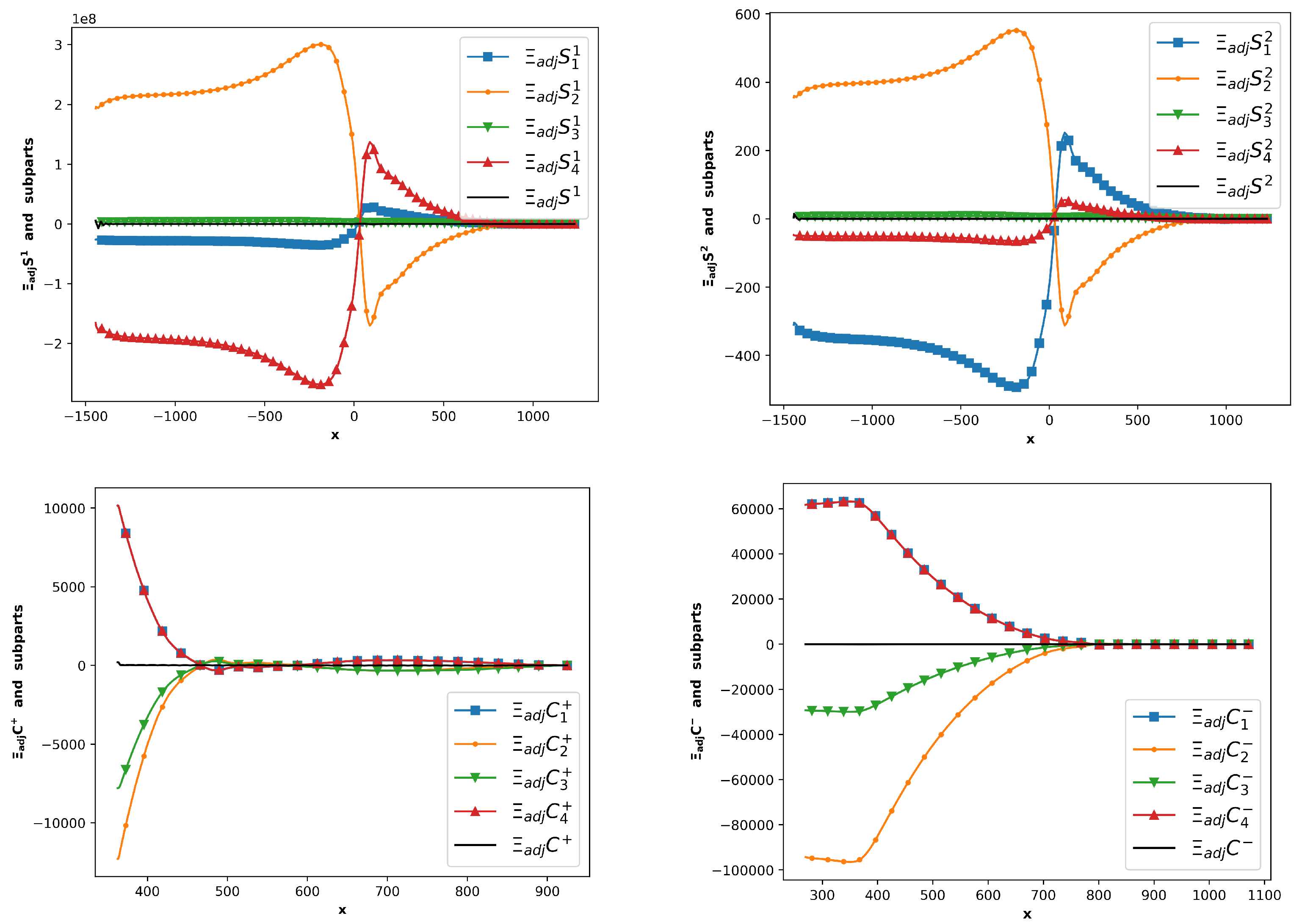
As in Section 4.3, the CEs are numerically assessed by checking that , , and are much smaller than their subterms all along the characteristic curves. This property is actually well satisfied, as can be seen in Figure 8. The error per series of curves, as defined in the previous subsection, has been calculated: 1.8 × 10 for , 2.6 × 10 for , 2.0 × 10 for , and 9.5 × 10 for .
5. Conclusions
The well-known equations satisfied in 2D inviscid flows along trajectories and in supersonic zones along C and C, are very helpful for the understanding of Mach waves, shockwaves, rarefaction waves, and nozzle flows. In this paper it has been shown that these equations can be derived using the conservative variables in a Cartesian frame of reference. This is in contrast to the canonical demonstrations in which the primitive variables are used in a frame of reference relative to the axis of motion.
In this work the study of the characteristic equations of the adjoint Euler equations has been continued, in particular using linear algebra arguments that simplify the discussion of the number of independent equations satisfied along the C and C, also deriving consequences of the characteristic equations relative to the adjoint components of the density and total energy equations. Of course, most of the efforts in CFD are devoted today to RANS, LES, and DNS flows. However, exact equations for Euler adjoint fields satisfied along trajectories along C and C in supersonic zones or throughout the fluid domain are very valuable for code verification. In the case of a continuous adjoint scheme or dual consistent discrete adjoint, they may directly serve for code verification and even validation of an adjoint code module. In the case of a general discrete adjoint code, the assessment of numerical solutions with respect to exact continuous equations is also linked to the difficult question of adjoint consistency, about which little has been proved today.
Supplementary Materials
The following are available online at https://www.mdpi.com/article/10.3390/aerospace10090797/s1, three Python files checking the formulas of , , , . Two Maple files checking the rank of the differential forms along the S and C curves.
Author Contributions
Investigation, K.A. and J.P.; software, J.P.; validation, K.A. and O.A.; writing, J.P., K.A. and O.A.; formal analysis, K.A. All authors have read and agreed to the published version of the manuscript.
Funding
The nozzle considered in Section 4 was designed in the framework of the SENECA project that is funded by the European Union’s Horizon 2020 research and innovation program under grant agreement No. 101006742, project SENECA ((LTO) Noise and Emissions of Supersonic Aircraft). This work was partially supported by the SONICE project, granted by the French Directorate General for Civil Aviation (DGAC).
Data Availability Statement
The data that support the findings of this study may be shared. Each request will be examined in conjunction with the managers of SENECA projects.
Acknowledgments
elsA V5.0 used in Section 4 and Appendix C is ONERA-Safran property. The authors warmly thank Sébastien Heib, Sana Amri, Sébastien Bourasseau, Thomas Hennion, and Antoine Dumont for many fruitful discussions.
Conflicts of Interest
The autors declare no conflict of interest.
Appendix A
• The coefficients are expressed below
• The coefficients are expressed below
• The coefficients are expressed below
• The coefficients are expressed below
• The coefficients are expressed below
• The coefficients are expressed below
• The coefficients are expressed below
Appendix B
Let us prove the equivalence between (14) and (42) in the case of a C. Equation (14) reading
with
A series of simplifications leads to the shorter expression
Expressing p in primitive variables yields
In addition, Equation (42) reads
It appears that the coefficients of Equations (A1) and (A2) are proportional:
Appendix C. Assessment of the Thrust Adjoint via a Shape Optimization
The discrete adjoint of the thrust is assessed via a shape optimization. In order to improve the thrust of the nozzle, six shape parameters are defined as factors of the following functions that drive changes in the y-coordinates:
. The seven points defining the x-range of the six bumps are linearly distributed between the abscissa of the inlet () and the abscissa of the rear of the nozzle (). is equal to half of the height between the inside wall at the throat and the symmetry line.These functions allow the y-coordinates of the deformed meshes to be calculated from the design parameters and the coordinates in the original mesh. The formula
is applied point-wise and the x-coordinates in the deformed mesh are the same as in the original mesh.
In order to optimize the thrust, a steepest descent has been performed with a maximum allowed wall displacement of of the throat height at each step. The norm of the first adjoint gradient is with strong negative and components (this negative sign is because the thrust is negative when computed along the x-axis). The 1D-descent step is bounded by the geometric constraint. The resulting deformation is a significant enlargement of the throat—see Figure A1 and Figure A3. This first optimization step increases the thrust by .
Figure A1.
SENECA nozzle. Isolines of the Mach number for the deformed geometry at step 1.
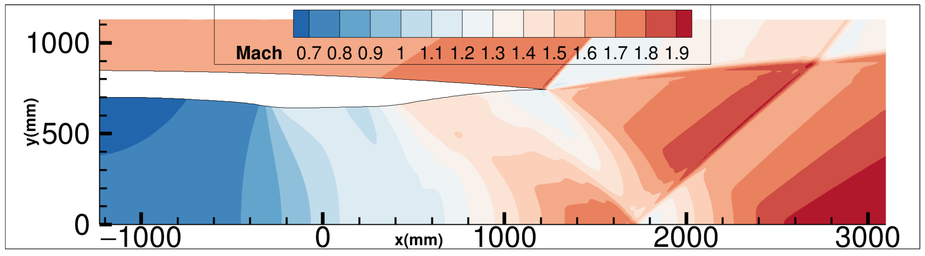
A second optimization step is performed. The norm of the thrust gradient is The displacement at this step is fixed by the 1D search of an optimum in the direction of the adjoint gradient. The nozzle is slightly enlarged in the inlet part—see Figure A2 and Figure A3. The thrust is increased by .
Figure A2.
SENECA nozzle. Isolines of the Mach number for the deformed geometry at step 2.
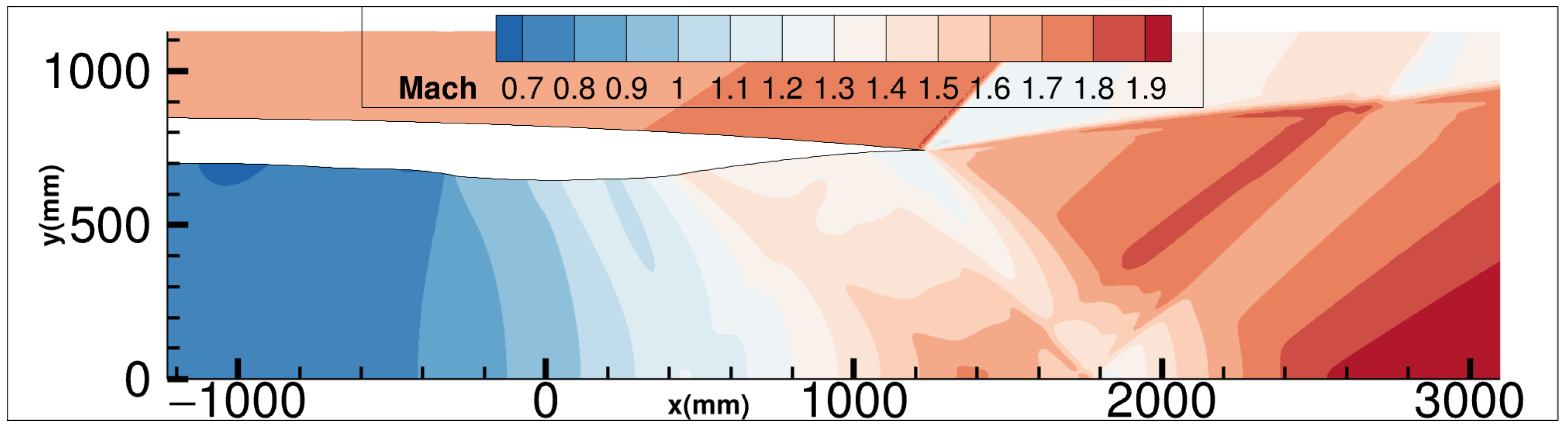
Figure A3.
SENECA nozzle. Inside wall shapes at the different steps: red, initial geometry; blue, after the first optimization step; black, after the second optimization step.
Figure A3.
SENECA nozzle. Inside wall shapes at the different steps: red, initial geometry; blue, after the first optimization step; black, after the second optimization step.

Finally, we check the consistency of our results with the classical formulas for a quasi-1D convergent–divergent “de Laval” nozzle. The thrust for such a configuration is expressed as
where is the mass flow. With a fixed stagnation state at the inlet and a value of significantly higher than 1, we expect the thrust to be optimized only via an increase of the mass flow.
In addition, the quasi-1D nozzle flows are calculated from the well-known equation expressing the mass flow as a function of the local section and the corresponding Mach number:
For the series of flows we consider, with at the throat and a fixed stagnation state at the inlet, a consequence of Equation (A6) is that the only way to increase the mass flow is to increase the throat section. This was achieved by the performed optimization, which increased the nozzle throat and the mass flow and, as a consequence, the thrust (more precisely, the mass flow was increased by with respect to its nominal value at the first optimization step and then by an additional at the second step).
References
- Ferri, A. Application of the Method of Characteristics to Supersonic Rotational Flow; TR 841; NASA: Washington, DC, USA, 1946. [Google Scholar]
- Shapiro, A. The Dynamics and Thermodynamics of Compressible Fluid Flow; The Ronald Press Company: New York, NY, USA, 1954. [Google Scholar]
- Bonnet, A.; Luneau, J. Aérodynamique. Théories de la Dynamique des Fluides; Cepadues: Toulouse, France, 1989. [Google Scholar]
- Délery, J. Traité D’aérodynamique Compressible; Collection Mécanique des Fluides, Lavoisier—Hermés, Science: Cachan, France, 2008; Volume 3. [Google Scholar]
- Jameson, A. Aerodynamic design via control theory. J. Sci. Comput. 1988, 3, 233–260. [Google Scholar] [CrossRef]
- Brezillon, J.; Gauger, N. 2D and 3D Aerodynamic Shape Optimization Using the Adjoint Aproach. Aerosp. Sci. Technol. J. 2004, 8, 715–727. [Google Scholar] [CrossRef]
- Brezillon, T.; Dwight, R. Discrete adjoint of the Navier-Sotkes equations for aerodynamic shape optimization. In Proceedings of the EUROGEN 2005, Munich, Germany, 12–14 September 2005. [Google Scholar]
- Peter, J.; Dwight, R. Numerical sensitivity analysis for aerodynamic optimization: A survey of approaches. Comput. Fluids 2010, 39, 373–391. [Google Scholar] [CrossRef]
- Schmidt, S.; Ilic, C.; Schultz, V.; Gauger, N. Three dimensional large scale aerodynamic shape optimization based on shape calculus. AIAA J. 2013, 51, 2615–2627. [Google Scholar] [CrossRef]
- Venditti, D.; Darmofal, D. Grid adaptation for functional outputs: Application to two-dimensional inviscid flows. J. Comput. Phys. 2002, 176, 40–69. [Google Scholar] [CrossRef]
- Dwight, R. Heuristic a posteriori estimation of error due to dissipation in finite volume schemes and application to mesh adaptation. J. Comput. Phys. 2008, 227, 2845–2863. [Google Scholar] [CrossRef]
- Todarello, G.; Vonck, F.; Bourasseau, S.; Peter, J.; Désidéri, J.A. Finite-volume goal-oriented mesh-adaptation using functional derivative with respect to nodal coordinates. J. Comput. Phys. 2016, 313, 799–819. [Google Scholar] [CrossRef]
- Giles, M.; Duta, M.; Müller, J.D. Adjoint code developments using the exact discrete approach. In Proceedings of the 15th AIAA Computational Fluid Dynamics Conference, Anaheim, CA, USA, 11–14 June 2001. AIAA Paper Series, Paper 2001-2596. [Google Scholar]
- Giles, M.; Duta, M.; Müller, J.D.; Pierce, N. Algorithm developments for discrete adjoint methods. AIAA J. 2003, 41, 198–205. [Google Scholar] [CrossRef]
- Economon, T.; Alonso, J.; Albring, T.; Gauger, N. Adjoint Formulation Investigations of Benchmark Aerodynamic Design Cases in SU2. In Proceedings of the 35th AIAA Applied Aerodynamics Conference, Denver, CO, USA, 5–9 June 2017. AIAA Paper Series, Paper 2017-4363. [Google Scholar]
- Sagebaum, M.; Albring, T.; Gauger, N. High-Performance Derivative Computations using CoDiPack. ACM Trans. Math. Softw. 2019, 45, 1–26. [Google Scholar] [CrossRef]
- Pinel, X.; Montagnac, M. Block Krylov methods to solve adjoint problems in aerodynamic design optimization. AIAA J. 2013, 51, 2183–2189. [Google Scholar] [CrossRef]
- Xu, S.; Radford, D.; Meyer, M.; Müller, J.D. Stabilisation of discrete steady adjoint solvers. J. Comput. Phys. 2015, 299, 175–195. [Google Scholar] [CrossRef]
- Lions, J.L. Contrôle Optimal de Systèmes Gouvernés par des Équations aux Derivées Partielles; Etudes Mathématiques; Dunod, Gauthier-Villars: Paris, France, 1968. [Google Scholar]
- Sartor, F.; Mettot, C.; Sipp, D. Stability, Receptivity, and Sensitivity Analyses of Buffeting Transonic Flow over a Profile. AIAA J. 2015, 53, 1980–1993. [Google Scholar] [CrossRef]
- Laurenceau, J. Surfaces de réponses par Krigeage pour l’optimisation de formes. Ph.D. Thesis, Institut National Polytechnique de Toulouse, Toulouse, France, 2008. [Google Scholar]
- de Baar, J.; Scholcz, T.; Dwight, R. Technical Note: Exploiting Adjoint Derivatives in High-Dimensional Metamodels. AIAA J. 2015, 53, 1391–1395. [Google Scholar] [CrossRef]
- Sipp, D.; Marquet, O.; Meliga, P.; Barbagallo, A. Dynamics and Control of Global Instabilities in Open-Flows: A Linearized Approach. Appl. Mech. Rev. 2010, 63, 030801. [Google Scholar] [CrossRef]
- Luchini, P.; Bottaro, A. Adjoint Equations in Stability Analysis. Annu. Rev. Fluid Mech. 2014, 46, 493–517. [Google Scholar] [CrossRef]
- Parish, E.; Duraisamy, K. A paradigm for data-driven predictive modeling using field inversion and machine learning. J. Comput. Phys. 2016, 305, 758–774. [Google Scholar] [CrossRef]
- Talagrand, O.; Courtier, P. Variational Assimilation of Meteorological Observations With the Adjoint Vorticity Equation. I: Theory. Q. J. R. Meteorol. Soc. 1987, 113, 1311–1328. [Google Scholar] [CrossRef]
- Hirsch, C. Numerical Computation of Internal and External Flows: The Fundamentals of Computational Fluid Dynamics, 2nd ed.; Butterworth—Heineman; Elsevier: Amsterdam, The Netherlands, 2007. [Google Scholar]
- Anderson, W.; Venkatakrishnan, V. Adjoint design optimization on unstructured grid using a continuous adjoint formulation. Comput. Fluids 1999, 28, 443–480. [Google Scholar] [CrossRef]
- Giles, M.; Pierce, N. Analytic adjoint solutions for the quasi-one-dimensional Euler equations. J. Fluid Mech. 2001, 426, 327–345. [Google Scholar] [CrossRef]
- Peter, J.; Désidéri, J.A. Ordinary differential equations for the adjoint Euler equations. Phys. Fluids 2022, 34, 086113. [Google Scholar] [CrossRef]
- Meyer, R.; Goldstein, S. The method of characteristics for problems of compressible flow involving two independant variables: Part I. The general theory. Q. J. Mech. Appl. Math. 1948, 1, 196–219. [Google Scholar] [CrossRef]
- Anderson, J. Modern Compressible Flow, 3rd ed.; McGraw-Hill Series in Aernautical and Aerospace Engineering; McGraw-Hill: New York, NY, USA, 2003. [Google Scholar]
- Oberkampf, W.; Trucano, T. Verification and validation in computational fluid dynamics. Prog. Aerosp. Sci. 2002, 38, 209–272. [Google Scholar] [CrossRef]
- Liepmann, H.; Roshko, A. Elements of Gasdynamics; Dover Publications: Mineola, NY, USA, 1956. [Google Scholar]
- Grossman, B. Fundamental Concepts of Real Gasdynamics; Virginia Polytechnic Institute and State University: Blacksburg, VA, USA, 2000. [Google Scholar]
- Mourouzidis, C. Preliminary Design of Next Generation Mach 1.6 Supersonic Business Jets to Investigate Landing and Take-Off (LTO) Noise and Emissions. In Proceedings of the 12th EASN conference on Innovation and Space for opening New Horizons, Barcelona, Spain, 18–21 October 2022. [Google Scholar]
- Cambier, L.; Heib, S.; Plot, S. The elsA CFD software: Input from research and feedback from industry. Mech. Ind. 2013, 14, 159–174. [Google Scholar] [CrossRef]
- Jameson, A.; Schmidt, W.; Turkel, E. Numerical Solutions of the Euler Equations by Finite Volume Methods Using Runge-Kutta Time-Stepping Schemes. In Proceedings of the 14th Fluid and Plasma Dynamics Conference, Palo Alto, CA, USA, 23–25 June 1981. AIAA Paper Series, Paper 1981-1259. [Google Scholar]
- Peter, J.; Renac, F.; Dumont, A.; Méheut, M. Discrete adjoint method for shape optimization and mesh adaptation in the elsA code. In Status and Challenges. In Proceedings of the 50th 3AF Symposium on Applied Aerodynamics, Toulouse, France, 29 March–1 April 2015. [Google Scholar]
- Peter, J.; Renac, F.; Labbé, C. Analysis of finite-volume discrete adjoint fields for two-dimensional compressible Euler flows. J. Comput. Phys. 2022, 449, 110811. [Google Scholar] [CrossRef]
- Giles, M.; Pierce, N. Adjoint equations in CFD: Duality, boundary conditions and solution behaviour. In Proceedings of the 13th Computational Fluid Dynamics Conference, Snowmass Village, CO, USA, 29 June–2 July 1997. AIAA Paper Series, Paper 97-1850. [Google Scholar]
- Lozano, C. On mesh sensitivities and boundary formulas for discrete adjoint-based gradients in inviscid aerodynamic shape optimization. J. Comput. Phys. 2017, 346, 403–436. [Google Scholar] [CrossRef]
- Lozano, C. Singular and discontinuous solutions of the adjoint Euler equations. AIAA J. 2018, 56, 4437–4451. [Google Scholar] [CrossRef]
- Lozano, C. Watch your adjoints! Lack of mesh convergence in inviscid adjoint solutions. AIAA J. 2019, 57, 3991–4006. [Google Scholar] [CrossRef]
- Peter, J. Contributions to Discrete Adjoint Method in Aerodynamics for Shape Optimization and Goal-Oriented Mesh Adaptation; University of Nantes. Mémoire pour Habilitation à Diriger des Recherches: Nantes, France, 2020. [Google Scholar]
Figure 1.
SENECA nozzle: fluid domain and boundary conditions diagram.
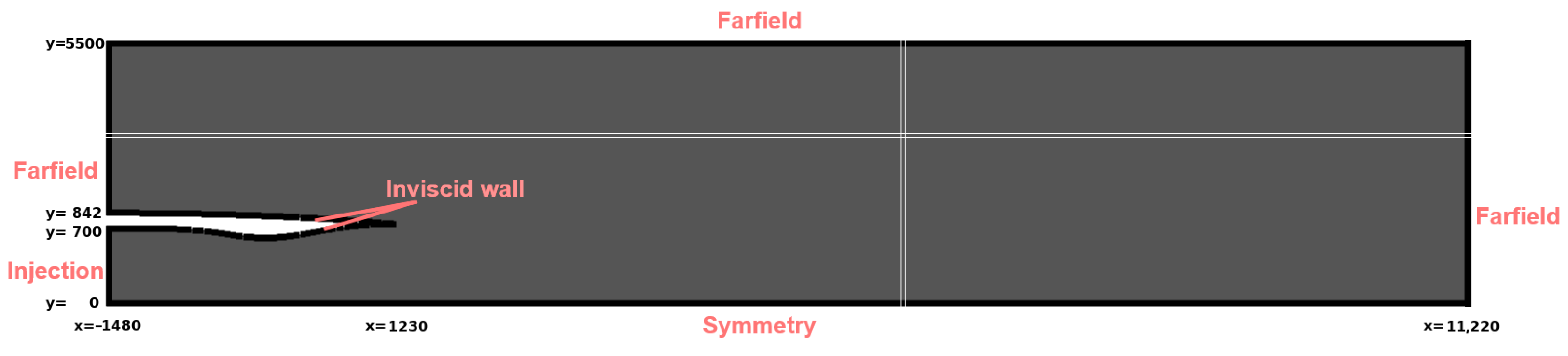
Figure 2.
SENECA nozzle. Green curve: C passing by the trailing edge of the nozzle. Dark gray zone: zone of the flow influencing the thrust .
Figure 2.
SENECA nozzle. Green curve: C passing by the trailing edge of the nozzle. Dark gray zone: zone of the flow influencing the thrust .

Figure 3.
SENECA nozzle. Isolines of Mach number (with Mach numbers in [1.9, 2.0] in white) vs. isolines of static pressure. Including selected C in green and C in purple for detailed flow analysis.
Figure 3.
SENECA nozzle. Isolines of Mach number (with Mach numbers in [1.9, 2.0] in white) vs. isolines of static pressure. Including selected C in green and C in purple for detailed flow analysis.

Figure 4.
SENECA nozzle. Isolines of Mach number. Selected S (in black), C (in green), and C (in purple) for the validation of the DCEs and ACEs. The thicker S (in dark gray) delimits the internal and the external flow.
Figure 4.
SENECA nozzle. Isolines of Mach number. Selected S (in black), C (in green), and C (in purple) for the validation of the DCEs and ACEs. The thicker S (in dark gray) delimits the internal and the external flow.
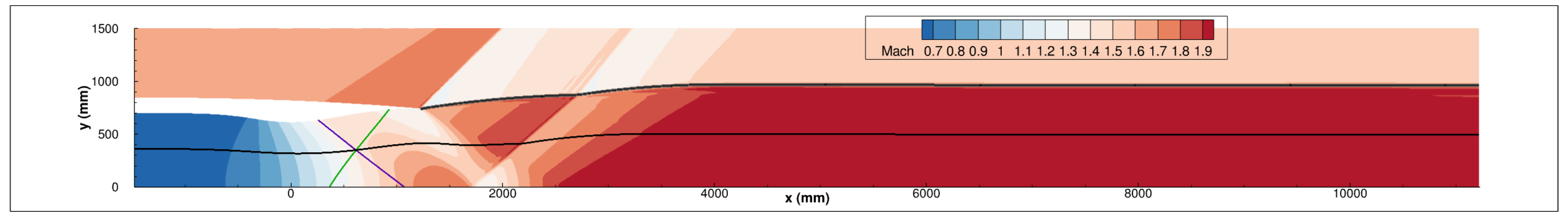
Figure 5.
SENECA nozzle. Isolines of the discrete adjoint of the thrust, component (dual of the mass-flow residual).
Figure 5.
SENECA nozzle. Isolines of the discrete adjoint of the thrust, component (dual of the mass-flow residual).
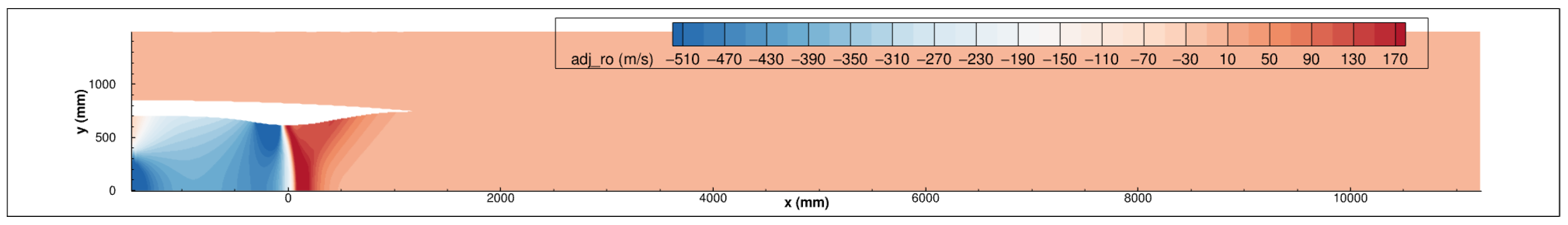
Figure 6.
SENECA nozzle. Isolines of (left) and H (right) with same levels.

Figure 7.
Numerical assessment of DCE (42). (left), (right) and their subparts integrated along the selected CC. Method of verification: the black curve should ideally coincide with the x-axis.
Figure 7.
Numerical assessment of DCE (42). (left), (right) and their subparts integrated along the selected CC. Method of verification: the black curve should ideally coincide with the x-axis.
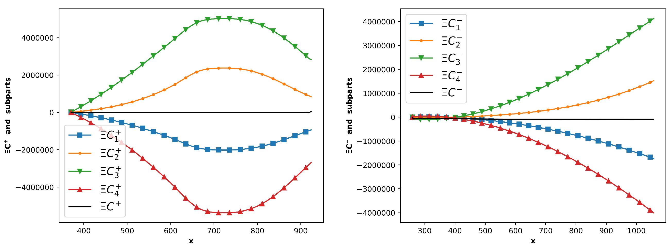
Figure 8.
Numerical assessment of the ACEs [30]. (upper left), (upper right), (bottom left), (bottom right) and their subparts integrated along the selected S, C, and C. Method of verification: the black curve should ideally coincide with the x-axis.
Figure 8.
Numerical assessment of the ACEs [30]. (upper left), (upper right), (bottom left), (bottom right) and their subparts integrated along the selected S, C, and C. Method of verification: the black curve should ideally coincide with the x-axis.
Disclaimer/Publisher’s Note: The statements, opinions and data contained in all publications are solely those of the individual author(s) and contributor(s) and not of MDPI and/or the editor(s). MDPI and/or the editor(s) disclaim responsibility for any injury to people or property resulting from any ideas, methods, instructions or products referred to in the content. |
© 2023 by the authors. Licensee MDPI, Basel, Switzerland. This article is an open access article distributed under the terms and conditions of the Creative Commons Attribution (CC BY) license (https://creativecommons.org/licenses/by/4.0/).
Share and Cite
MDPI and ACS Style
Ancourt, K.; Peter, J.; Atinault, O. Adjoint and Direct Characteristic Equations for Two-Dimensional Compressible Euler Flows. Aerospace 2023, 10, 797. https://doi.org/10.3390/aerospace10090797
AMA Style
Ancourt K, Peter J, Atinault O. Adjoint and Direct Characteristic Equations for Two-Dimensional Compressible Euler Flows. Aerospace. 2023; 10(9):797. https://doi.org/10.3390/aerospace10090797
Chicago/Turabian StyleAncourt, Kevin, Jacques Peter, and Olivier Atinault. 2023. "Adjoint and Direct Characteristic Equations for Two-Dimensional Compressible Euler Flows" Aerospace 10, no. 9: 797. https://doi.org/10.3390/aerospace10090797
Note that from the first issue of 2016, this journal uses article numbers instead of page numbers. See further details here.