DDPG-Based Convex Programming Algorithm for the Midcourse Guidance Trajectory of Interceptor

Abstract

To address the problem of low accuracy and efficiency in trajectory planning algorithms for interceptors facing multiple constraints during the midcourse guidance phase, an improved trajectory convex programming method based on the lateral distance domain is proposed. This algorithm can achieve fast trajectory planning, reduce the approximation error of the planned trajectory, and improve the accuracy of trajectory guidance. First, the concept of lateral distance domain is proposed, and the motion model of the midcourse guidance segment in the interceptor is converted from the time domain to the lateral distance domain. Second, the motion model and multiple constraints are convexly and discretely transformed, and the discrete trajectory convex model is established in the lateral distance domain. Third, the deep reinforcement learning algorithm is used to learn and train the initial solution of trajectory convex programming, and a high-quality initial solution trajectory is obtained. Finally, a dynamic adjustment method based on the distribution of approximate solution errors is designed to achieve efficient dynamic adjustment of grid points in iterative solving. The simulation experiments show that the improved trajectory convex programming algorithm proposed in this paper not only improves the accuracy and efficiency of the algorithm but also has good optimization performance.

1. Introduction

In actual combat, to maximize intercept effectiveness, the interceptor system seeks to reduce the response time from the detection system’s detection of the target to the launch of the interceptor. Moreover, as the longest duration part of the combined guidance process, the trajectory design of the midcourse guidance section largely determines the terminal intercept capability of the interceptor and is a key factor in determining the success or failure of the intercept mission. At the same time, the trajectory planning problem in the midcourse guidance phase is a complex non-linear problem with multiple constraints, which requires the overall consideration of physical constraints, such as dynamic pressure, overload, and thermal flow density during the flight process, while ensuring that the terminal constraints are met. Therefore, this problem places high demands on the accuracy and efficiency of the midcourse guidance trajectory optimization algorithm.

In addition to satisfying certain constraints, trajectory planning also requires finding a particular trajectory, which satisfies some performance indices from the initial position to the target position [1]. Currently, the previous method used in the study of such problems for their solution is the indirect method. In Ref [2], the analytical solution of the shooting equation for the on-line trajectory optimization problem of planetary landing is derived, and the indirect method is improved by combining the homotopy theory technology to achieve an optimal propellant. Grant and Braun [3] design a fast trajectory optimization method by combining indirect optimization, continuation, and symbolic manipulation theories. Shen et al. [4] propose an optimization method combining the indirect method and homotopy approach for solving an impulse trajectory. In the research of dealing with the problem of difficult selection of the initial values of co-state variables in indirect methods, Lee et al. [5] propose a non-functional approximation or extrapolation initial guess structure to deal with specific energy targeting problems. Ren et al. [6] simplify the dynamic model and, based on it, design an initial guess generator with high computational efficiency, which allows the initial value to be obtained by analytically solving a linear system of equations. For the trajectory optimization problem, the indirect method not only has the advantage of high computational accuracy, but it also theoretically proves the optimality of the optimized trajectory. However, the difficulty in selecting the initial values of the co-state variables has not been fully solved, which severely limits the development and application of the indirect method.

The principle of the direct method of problem solving is different from that of the indirect method. It discretizes the problem, which makes the procedure for solving the problem simple and avoids the inaccuracy of the initial value solution in indirect methods. It has been widely applied to the solution of optimal trajectory problems [7,8,9,10]. Especially in recent years, with the significant improvement in scientific computing hardware capabilities, the pseudospectral method, as a typical method of point collocation in direct methods, has been widely applied by researchers to solve trajectory planning problems, and its theory has been improved and extended [11,12]. Zhang et al. [13] design a multi-objective globally optimal homing trajectory for a wing parachute based on the Gaussian pseudospectral method. Zhang et al. [14] propose an improved Radau pseudospectral method combined with deep neural networks to solve the chase and escape game problem of orbital trajectory. Li et al. [15] propose a hybrid optimization method based on the conjugate gradient method and pseudospectral point matching method for the optimal trajectory planning problem during rocket landing. However, all types of pseudospectral methods have the problem of imprecise efficiency solution accuracy, which is a major obstacle to their application in practical engineering.

In addition, intelligent optimization algorithms are often used to solve trajectory planning generation problems due to their ability to effectively handle complex multi-constraint and multi-dimensional optimization problems [16,17]. Zhao et al. [18] generate reliable constrained glide trajectories for hypersonic gliding vehicles by improving the pigeon inspired optimization (PIO) algorithm. Duan et al. [19] combine the direct collocation method and the artificial bee colony algorithm to optimize and generate the re-entry trajectory of hypersonic aircraft. Zhou et al. [20] establish a dynamic pressure profile-based optimization model for the hypersonic vehicle trajectory optimization problem, transform the problem into a parameter optimization problem, and solve it using an improved particle swarm optimization algorithm. Li et al. [21] propose an improved particle swarm optimization algorithm combined with gradient search to solve the problem of rapid re-entry trajectory optimization of a hypersonic glider—which solves the problem of insufficient accuracy due to early convergence of the algorithm—and apply it to problem solving. Gaudet et al. [22] combine the adaptability of reinforcement learning and the fast learning ability of meta learning, proposing a missile guidance and control method based on reinforcement meta learning. D’Ambrosio et al. [23] combine the Pontryagin maximum principle with the powerful learning ability of neural networks to propose a fuel optimal trajectory learning method based on the Pontryagin neural network. However, intelligent optimization algorithms face the problem of falling into local optima. How to avoid this problem is a key issue, which needs to be addressed in current research.

In recent years, convex optimization methods have become a powerful tool in aircraft trajectory planning research due to their fast solution speed and ability to handle constrained problems [24,25,26]. In Ref [27], for the optimal guidance problem of planetary orbit insertion, the problem is transformed into a convex optimization problem through constrained convex relaxation, linearization, and discretization, and a convex optimization algorithm based on the interior point method is proposed. Based on convex optimization methods, Liu et al. [28] propose a regularization technique to ensure the accuracy of convex relaxation and solve the optimal terminal guidance problem of aerodynamic control missiles. Cheng et al. [29] accelerate the efficiency of the convex optimization algorithm to solve the trajectory planning problem of the ascent phase of the launch vehicle by using the Newton–Kantorovich/pseudospectral method to iteratively solve the initial solution. In Ref [30], for the aircraft re-entry guidance problem, the continuous linearization and convexification techniques are used to transform the problem into a continuous convex programming problem, and a convex optimization re-entry guidance method is designed to solve the problem, which reduces the sensitivity of the initial guess accuracy. Zhou et al. [31] improve the efficiency and accuracy of the algorithm by designing a dynamic adjustment grid point method based on the original sequence convex programming algorithm. In Ref [32], a pseudospectral convex optimization technology combining the advantages of the pseudospectral method and convex optimization is proposed to achieve optimal trajectory planning during rocket power descent and landing processes. On the basis of the pseudospectral convex optimization technology framework, Sagliano et al. [33,34,35] further propose the generalized hp pseudospectral convex programming method and the lobatto pseudospectral convex programming method, which improve the flexibility and efficiency of the algorithm optimization process. Song et al. [36] propose an adaptive dynamic descent guidance method based on multi-stage pseudospectral convex optimization, which achieves adaptive trajectory planning during rocket landing. The above methods all perform convex transformation on the aircraft motion equation and constraints in the time domain, which achieves the optimization and generation of the aircraft trajectory. However, the relationship between the grid point position and the physical position of the target in the time domain is not intuitive, which makes it difficult to analyze the approximation error of the trajectory. In addition, using convex optimization algorithms to solve trajectory optimization problems requires feasible trajectories, which satisfy the constraints to be used as initial solutions; otherwise, the algorithm may not find the optimal approximate solution for a long time, or it may even diverge. This problem also greatly hinders the performance improvement and application of convex optimization algorithms.

This paper addresses the problem of rapid trajectory optimization generation in the guidance phase of an interceptor under multiple constraints. In terms of problem model processing, the motion model and multiple constraints are transformed into convex and discrete forms, allowing the optimization problem to be transformed into a sequential convex programming problem, which can be solved using convex optimization methods. The problem model is also transformed from the time domain to the lateral distance domain, which describes the positional relationship more intuitively. In terms of generating initial solution trajectories, this paper uses the deep deterministic policy gradient (DDPG) algorithm to train the planning generation of interceptor midcourse guidance trajectories, obtaining high-quality initial solution trajectories, which satisfy the basic guidance requirements, and improving the generation speed and guidance accuracy of optimized trajectories. In terms of the adjustment of dynamic grid point, this paper uses the distribution of grid point approximation error to determine the dynamic adjustment of grid points and adjust them to the appropriate position, thereby reducing the approximation error of the optimized trajectory and improving the solving efficiency of the convex optimization algorithm. The main contributions can be summarized as follows:

(1).

On the lateral plane of the three-dimensional trajectory, based on the lateral range of the interceptor, the concept of the lateral distance domain is proposed, which transforms the problem model from the time domain to the horizontal distance domain, simplifies the convexification of the problem model, and facilitates the analysis of the approximation error.

(2).

Based on the characteristics of the trajectory planning model in the mid-guidance phase, the corresponding Markov decision process (MDP) is designed, and the DDPG algorithm is applied to learn and train the initial solution trajectory planning task, and a higher quality initial solution trajectory is obtained.

(3).

The dynamic adjustment strategy of grid points in the convex optimization algorithm is improved. In the iterative solution process, the position distribution of grid points is adjusted based on the distribution of approximate solution errors of grid points, which not only reduces the approximate solution error of the whole optimization trajectory but also improves the efficiency of the algorithm.

The sections of this paper are structured as follows. This first section briefly analyzes the state of the art in trajectory optimization generation algorithms and outlines the main contributions of this paper. In the second section, the problem of optimizing the midcourse guidance trajectory of the interceptor is described. The third section describes the convexity and discretization of the problem. In the fourth section, the fast method for generating initial solution trajectories based on the DDPG algorithm is presented. In the fifth section, the grid point dynamic adjustment method based on the approximate solution error distribution is designed. In the sixth section, the research content is simulated and verified. In the last section, the content of this paper is summarized.

2. Problem Description

2.1. Model Establishment

To facilitate the trajectory calculation, the numerical values are normalized, and the interceptor’s guidance motion model is processed dimensionless. The dimensionless target motion equation [36] is given by

$$\left\{\begin{array}{l}dh/dt=v\sin \theta \\ dz/dt=v\cos \theta \sin {\psi }_v\\ dx/dt=v\cos \theta \cos {\psi }_v\\ dv/dt=-D_{\alpha }-g\sin \theta \\ d\theta /dt=L_{\alpha }\cos \sigma /v-g\cos \theta /v\\ d{\psi }_v/dt=L_{\alpha }\sin \sigma /v\cos \theta \\ d\alpha /dt=\dot{\alpha }\\ d\sigma /dt=\dot{\sigma }\end{array}\right.$$

(1)

where h, z, and x are the dimensionless position of the centroid of the interceptor under the northeastern sky coordinate system; v is the dimensionless velocity of the interceptor; θ is the angle of inclination of the trajectory; ψ_v is the angle of deflection of the trajectory; α is the angle of attack; σ is the angle of bank; D_α, L_α, g are the dimensionless drag, lift, and gravitational acceleration of the interceptor, and their calculation formulae are as follows:

$$\left\{\begin{array}{l}{D}_{\alpha }=C_{D}pS/m\\ L_{\alpha }=C_{L}pS/m\\ g=g_0{\left(1/(1+h)\right)}^2\end{array}\right.$$

(2)

where p is the dynamic pressure; S is the characteristic area of the interceptor; m is the mass of the interceptor; g₀ is the acceleration of gravity at sea level, and its value is 9.81 m/s²; C_D and C_L are the coefficients of drag and lift, respectively, which can be expressed as a function of α:

$$\left\{\begin{array}{l}{C}_D=c_{d1}+c_{d2}\alpha +c_{d3}{\alpha }^2\\ C_L=c_{l1}+c_{l2}\alpha \end{array}\right.$$

(3)

where c_d1, c_d2, and c_d3 are the drag parameters; c_l1 and c_l2 are the lift parameters. The calculation of p is as follows:

$$p=0.5\rho {(v\sqrt{g_0{r}_e})}^2$$

(4)

where r_e is the earth’s radius, and it is 6371.2 km; ρ is the air density, and its calculation formula is as follows:

$$\rho ={\rho }_0{e}^{-h{r}_e/H}$$

(5)

where ρ₀ is the air density at sea level, and it is 1.266 km/m³; H is the reference height, and it is 7254.24 m. The linear distance l between the interceptor and the target in the transverse plane is defined as

$$l=\sqrt{{(x-x_0)}^2+{(z-z_0)}^2}$$

(6)

where x₀ and z₀ are the initial values representing the initial value of the position coordinate. The linear velocity v_l of the interceptor in the transverse plane is

$$v_l=dl/dt=v\cos \theta \cos ({\psi }_l-{\psi }_v)$$

(7)

where ψ_l is the angle of the line of sight of the missile and the target in the transverse plane, expressed as

$${\psi }_l=\arccos \left((z_f-z)/\sqrt{{(z_f-z)}^2+{(x_f-x)}^2}\right)$$

(8)

where x_f and z_f are the final values of the position coordinate.

Given the initial and final positions of the interceptor in the xOz plane, as shown in Figure 1, each grid point position of the planned trajectory in the lateral distance has a corresponding point on its linear distance. When the grid point positions of the planned trajectory are determined, their lateral distance and linear distance expressions can be converted to each other, i.e., the lateral distance of the planned trajectory can be expressed as the superposition of the segmented distances of the initial and final positions of the interceptor in the linear direction. This can visually reflect the physical relationship between the grid point positions and the terminal positions, which is useful for analyzing the approximation error of the trajectory.

The model Equation (1) is transformed by Equation (7) to obtain the midcourse guidance motion model in the lateral distance domain as follows:

$$\left\{\begin{array}{l}dh/dl=\tan \theta /\cos ({\psi }_l-{\psi }_v)\hfill \\ dz/dl=\sin {\psi }_v/\cos ({\psi }_l-{\psi }_v)\hfill \\ dx/dl=\cos {\psi }_v/\cos ({\psi }_l-{\psi }_v)\hfill \\ dv/dl=-D/\left(v\cos \theta \cos ({\psi }_l-{\psi }_v)\right)-\tan \theta /\left({(1+h)}^{2}v\cos ({\psi }_l-{\psi }_v)\right)\hfill \\ d\theta /dl=L\cos \sigma /\left(v^2\cos \theta \cos ({\psi }_l-{\psi }_v)\right)-1/\left({(1+h)}^2{v}^2\cos ({\psi }_l-{\psi }_v)\right)\hfill \\ \begin{array}{l}d{\psi }_v/dl=L\sin \sigma /\left(v^2{\cos }^2\theta \cos ({\psi }_l-{\psi }_v)\right)\\ d\alpha /dl=\dot{\alpha }\\ d\sigma /dl=\dot{\sigma }\end{array}\hfill \end{array}\right.$$

(9)

2.2. Problem Formulation

According to the model analysis in Section 2.1, the state equation of the interceptor can be expressed as

$$\dot{s}=f(s,l)+Bu(l) l\in [0,l_f]$$

(10)

$$f(s,l)=\left\{\begin{array}{l}\tan \theta /\cos ({\psi }_l-{\psi }_v)\hfill \\ \sin {\psi }_v/\cos ({\psi }_l-{\psi }_v)\hfill \\ \cos {\psi }_v/\cos ({\psi }_l-{\psi }_v)\hfill \\ -D/\left(v\cos \theta \cos ({\psi }_l-{\psi }_v)\right)-\tan \theta /\left({(1+h)}^{2}v\cos ({\psi }_l-{\psi }_v)\right)\hfill \\ L\cos \sigma /\left(v^2\cos \theta \cos ({\psi }_l-{\psi }_v)\right)-1/\left({(1+h)}^2{v}^2\cos ({\psi }_l-{\psi }_v)\right)\hfill \\ L\sin \sigma /\left(v^2{\cos }^2\theta \cos ({\psi }_l-{\psi }_v)\right)\hfill \\ 0\hfill \\ 0\hfill \end{array}\right.$$

(11)

$$B={\left[\begin{array}{cccccccc}0& 0& 0& 0& 0& 0& 1& 0\\ 0& 0& 0& 0& 0& 0& 0& 1\end{array}\right]}^T$$

(12)

where s = [h, z, x, v, θ, ψ_v, α, σ] is the state variable of interceptor, and u = $[\dot{\alpha },\dot{\sigma }]$ is the control variable of interceptor. During the midcourse guidance phase, the interceptor flies at high altitude and high speed for a long time, which is subject to constraints on heat flux density Q, dynamic pressure p, overload n, angle, and control variables. Therefore, the following constraints should also be met [37].

$$\left\{\begin{array}{l}Q=C_Q{\rho }^{0.5}{(v\sqrt{g_0{r}_e})}^{3.05}\le Q_{\max }\\ p=0.5\rho {(v\sqrt{g_0{r}_e})}^2\le p_{\max }\\ n=\sqrt{L^2+D^2}{(1+h)}^2\le n_{\max }\end{array}\right.$$

(13)

$$\left\{\begin{array}{l}\left|\theta \right|\le {\theta }_{\max }\\ \left|{\psi }_v\right|\le {\psi }_{v\max }\\ \left|\alpha \right|\le {\alpha }_{\max }\\ \left|\sigma \right|\le {\sigma }_{\max }\end{array}\right.$$

(14)

$$\left\{\begin{array}{l}\left|\dot{\alpha }\right|\le {\dot{\alpha }}_{\max }\\ \left|\dot{\sigma }\right|\le {\dot{\sigma }}_{\max }\end{array}\right.$$

(15)

where C_Q = 1.291 × 10⁻⁴ is the computational constant of Q, and Q_max, p_max, n_max, θ_max, ψ_vmax, α_max, σ_max, $\dot{\alpha }$_max, $\dot{\sigma }$_max are the maximum limit value of constraints. The purpose of trajectory planning is to achieve guidance tasks under constraint conditions; therefore, the objective function of the problem can be written as

$$J_0=k_1\left({(z_f^{\ast }-z_f)}^2+{(x_f^{\ast }-x_f)}^2\right)+k_2{(h_f^{\ast }-h_f)}^2$$

(16)

where $x_f^{\ast },y_f^{\ast },z_f^{\ast }$ are the expected final position coordinates; k₁ and k₂ are the weighting coefficients. In summary, the problem of rapid optimization and generation of midcourse guidance trajectory can be expressed as

$$\begin{array}{l}{\mathrm{P}}_0:\min \hspace{1em}\hspace{1em}\hspace{1em} (16)\\ \hspace{1em} \mathrm{subject} \mathrm{to}: \left(10\right),\left(12\right),\left(13\right),\left(14\right),\left(15\right)\\ \hspace{1em}\hspace{1em}\hspace{1em}\hspace{1em}\hspace{1em}\hspace{1em} s(l=0)=[h_0,z_0,x_0,v_0,{\theta }_0,{\psi }_{v0},{\alpha }_0,{\sigma }_0]\\ \hspace{1em}\hspace{1em}\hspace{1em}\hspace{1em}\hspace{1em}\hspace{1em} v(l=l_f)\ge v_f\end{array}$$

(17)

3. Problem Convexity and Discretization Processing

In order to treat problem P₀ with a convex optimization approach, it is necessary to ensure that the equation constraints in problem P₀ are linear and that the objective function and inequality constraints are both convex and linear. However, the model equations and process constraints of problem P₀ are non-linear and are not convex optimization problems. Therefore, the following treatment is required before the convex optimization algorithm can be used to solve problem P₀.

3.1. Problem Convexity Processing

The motion model Equation (10) of the problem, as an equality constraint, must be linear in convex optimization problems. Therefore, it is necessary to linearize the non-linear part of Equation (10) in the problem, as shown below:

$$\dot{s}=f(s){|}_{s=s^k}+f(s{)}^{\prime }{|}_{s=s^k}(s-s^k)+Bu$$

(18)

Assuming A = $f(s{)}^{\prime }{|}_{s=s^k}$ and C = $f(s){|}_{s=s^k}-f(s{)}^{\prime }{|}_{s=s^k}{s}^k$, Equation (18) can be expressed as

$$\dot{s}=As+Bu+C$$

(19)

$$A=\left[\begin{array}{cccccccc}0& 0& 0& 0& a_{15}& a_{16}& 0& 0\\ 0& 0& 0& 0& 0& a_{26}& 0& 0\\ 0& 0& 0& 0& 0& a_{36}& 0& 0\\ a_{41}& 0& 0& a_{44}& a_{45}& a_{46}& a_{47}& 0\\ a_{51}& 0& 0& a_{54}& a_{55}& a_{56}& a_{57}& a_{58}\\ a_{61}& 0& 0& 0& a_{65}& a_{66}& a_{67}& a_{68}\\ 0& 0& 0& 0& 0& 0& 0& 0\\ 0& 0& 0& 0& 0& 0& 0& 0\end{array}\right]$$

(20)

$$\left\{\begin{array}{l}{a}_{41}=r_{e}D/\left(Hv\cos \theta \cos ({\psi }_l-{\psi }_v)\right)+2\tan \theta /\left({(1+h)}^{3}v\cos ({\psi }_l-{\psi }_v)\right)\hfill \\ a_{51}=-r_{e}L\cos \sigma /\left(H{v}^2\cos \theta \cos ({\psi }_l-{\psi }_v)\right)+2/\left({(1+h)}^3{v}^2\cos ({\psi }_l-{\psi }_v)\right)\hfill \\ a_{61}=-r_{e}L\sin \sigma /\left(H{v}^2{\cos }^2\theta \cos ({\psi }_l-{\psi }_v)\right)\hfill \end{array}\right.$$

(21)

$$\left\{\begin{array}{l}{a}_{44}=D/\left(v^2\cos \theta \cos ({\psi }_l-{\psi }_v)\right)+\tan \theta /\left({(1+h)}^2{v}^2\cos ({\psi }_l-{\psi }_v)\right)\hfill \\ a_{54}=2/\left({(1+h)}^2{v}^3\cos ({\psi }_l-{\psi }_v)\right)\hfill \end{array}\right.$$

(22)

$$\left\{\begin{array}{l}{a}_{15}=1/{\cos }^2\theta \cos ({\psi }_l-{\psi }_v)\hfill \\ a_{45}=-D\tan \theta /\left(v\cos \theta \cos ({\psi }_l-{\psi }_v)\right)-1/\left({(1+h)}^{2}v{\cos }^2\theta \cos ({\psi }_l-{\psi }_v)\right)\hfill \\ a_{55}=\tan \theta L\cos \sigma /\left(v^2\cos \theta \cos ({\psi }_l-{\psi }_v)\right)\hfill \\ a_{65}=2\tan \theta L\sin \sigma /\left(v^2{\cos }^2\theta \cos ({\psi }_l-{\psi }_v)\right)\hfill \end{array}\right.$$

(23)

$$\left\{\left\{\begin{array}{l}{a}_{16}=-\tan \theta \tan ({\psi }_l-{\psi }_v)/\cos ({\psi }_l-{\psi }_v)\hfill \\ a_{26}=\left(\cos {\psi }_v-\sin {\psi }_v\tan ({\psi }_l-{\psi }_v)\right)/\cos ({\psi }_l-{\psi }_v)\hfill \\ a_{36}=-\left(\sin {\psi }_v+\cos {\psi }_v\tan ({\psi }_l-{\psi }_v)\right)/\cos ({\psi }_l-{\psi }_v)\hfill \\ a_{46}=D\tan ({\psi }_l-{\psi }_v)/\left(v\cos \theta \cos ({\psi }_l-{\psi }_v)\right)\hfill \\ a_{56}=\left(\tan ({\psi }_l-{\psi }_v)/\left(v^2\cos ({\psi }_l-{\psi }_v)\right)\right)\left(1/{(1+h)}^2-L\cos \sigma /\cos \theta \right)\hfill \\ a_{66}=-\tan ({\psi }_l-{\psi }_v)L\sin \sigma /\left(v^2{\cos }^2\theta \cos ({\psi }_l-{\psi }_v)\right)\hfill \end{array}\right.\right.$$

(24)

$$\left\{\begin{array}{l}{a}_{47}=-\left((c_{d2}+2c_{d3})/(c_{d1}+c_{d2}\alpha +c_{d3}{\alpha }^2)\right)\left(D/\left(v\cos \theta \cos ({\psi }_l-{\psi }_v)\right)\right)\hfill \\ a_{57}=\left(c_{l2}/(c_{l1}+c_{l2}\alpha )\right)\left(L\cos \sigma /\left(v^2\cos \theta \cos ({\psi }_l-{\psi }_v)\right)\right)\hfill \\ a_{67}=\left(c_{l2}/(c_{l1}+c_{l2}\alpha )\right)\left(L\sin \sigma /\left(v^2{\cos }^2\theta \cos ({\psi }_l-{\psi }_v)\right)\right)\hfill \end{array}\right.$$

(25)

$$\left\{\begin{array}{l}{a}_{58}=-L\sin \sigma /\left(v^2\cos \theta \cos ({\psi }_l-{\psi }_v)\right)\hfill \\ a_{68}=L\cos \sigma /\left(v^2{\cos }^2\theta \cos ({\psi }_l-{\psi }_v)\right)\hfill \end{array}\right.$$

(26)

At the same time, to reduce the linearization error of the motion model, trust region constraints are added as follows:

$$\left|s-s^k\right|\le \delta$$

(27)

where δ is the trust region constraint radius, which is the same as the s dimension. The heat flow density, dynamic pressure, and overload constraint functions shown in Equation (13) are strongly non-linear and neither convex functions nor concave functions; therefore, it is still necessary to linearize these functions as follows:

$$\left\{\begin{array}{l}Q=Q^k+{\left.\partial Q/\partial h\right|}_{s=s^k}(h-h^k)+{\left.\partial Q/\partial v\right|}_{s=s^k}(v-v^k)\le Q_{\max }\hfill \\ p=p^k+{\left.\partial p/\partial h\right|}_{s=s^k}(h-h^k)+{\left.\partial p/\partial v\right|}_{s=s^k}(v-v^k)\le p_{\max }\hfill \\ n=n^k+{\left.\partial n/\partial h\right|}_{s=s^k}(h-h^k)+{\left.\partial n/\partial v\right|}_{s=s^k}(v-v^k)+{\left.\partial q/\partial \alpha \right|}_{s=s^k}(\alpha -{\alpha }^k)\le {\alpha }_{\max }\hfill \end{array}\right.$$

(28)

$$\left\{\begin{array}{l}{\left.\partial Q/\partial h\right|}_{s=s^k}=-r_e{\rho }^{0.5}{C}_Q{(v\sqrt{g_0{r}_e})}^{3.15}/2H\\ {\left.\partial Q/\partial v\right|}_{s=s^k}=3.15{\rho }^{0.5}{C}_Q{(v\sqrt{g_0{r}_e})}^{3.15}/v\end{array}\right.$$

(29)

$$\left\{\begin{array}{l}{\left.\partial q/\partial h\right|}_{s=s^k}=-r_e\rho C{v}^2{g}_0{r}_e/2H\\ {\left.\partial q/\partial v\right|}_{s=s^k}=\rho v{g}_0{r}_e\end{array}\right.$$

(30)

$$\left\{\begin{array}{l}{\left.\partial n/\partial h\right|}_{s=s^k}=(1+h)\sqrt{L^2+D^2}\left(2-r_e(1+h)/H\right)\hfill \\ {\left.\partial n/\partial v\right|}_{s=s^k}=2{(1+h)}^2\sqrt{L^2+D^2}/v\hfill \\ {\left.\partial n/\partial \alpha \right|}_{s=s^k}=\left((c_{l1}+c_{l2}\alpha )c_{l2}+(c_{d1}+c_{d2}\alpha +c_{d3}{\alpha }^2)(c_{d2}+c_{d3}\alpha )\right)\hfill \\ \hspace{1em}\hspace{1em}{(1+h)}^2\sqrt{L^2+D^2}/(C_L^2+C_D^2)\hfill \end{array}\right.$$

(31)

The objective function shown in Equation (16) is a convex function formed by the combination of an absolute value function and a linear function. In this paper, an additional term is added to Equation (16) in order to make the manipulated variable smoother and to avoid excessive amplitude oscillation.

$$J_1=J_0+k_3{\displaystyle {\int }_0^{l_f}\left|\dot{\alpha }\right|+\left|\dot{\sigma }\right|dl}$$

(32)

where k₃ is the weighting coefficient. In summary, problem P₀ can be transformed into a new convex problem P₁.

$$\begin{array}{l}{\mathrm{P}}_1:\min \hspace{1em}\hspace{1em}\hspace{1em}(32)\\ \hspace{1em} \mathrm{subject} \mathrm{to}:\left(19\right),\left(27\right),\left(28\right),\left(14\right),\left(15\right)\\ \hspace{1em}\hspace{1em}\hspace{1em}\hspace{1em}\hspace{1em}\hspace{1em} s(l=0)=[h_0,z_0,x_0,v_0,{\theta }_0,{\psi }_{v0},{\alpha }_0,{\sigma }_0]\\ \hspace{1em}\hspace{1em}\hspace{1em}\hspace{1em}\hspace{1em}\hspace{1em} v(l=l_f)\ge v_f\end{array}$$

(33)

3.2. Problem Discretization Processing

Problem P₁ is a convex optimization problem in a continuous distance domain, with continuous state and control variables, which makes it difficult to solve directly. It is necessary to transform it into a discrete mathematical programming problem with finite parameters for optimization, so that it can be solved by numerical methods.

Assuming that the position of the grid points on the generated trajectory in the lateral distance domain is li, i = 1, …, t represents the position sequence number of the grid points, and l₁ = 0 ≤ … ≤ l_i ≤ l_i+1 ≤… ≤ l_t = l_f. To keep the transcription process simple, the Euler method is used to discretize the equation of motion Equation (19).

$$s_{i+1}=s_i+\Delta l_i{\dot{s}}_i=s_i+\Delta l_i(As+Bu+C)$$

(34)

where △l_i is the position difference between grid points i and i + 1 in the lateral distance domain. After discretizing the motion equations, a similar discretization is applied to the constraints and objective function in problem P₁. Considering that the size of the trust region required for each iterative optimization solution may vary, this paper uses the variable trust region method to improve the convergence efficiency of the algorithm iteration.

$$\left|s_j-s_j^k\right|\le \lambda \odot \delta$$

(35)

where λ = [λ_h, λ_z, λ_x, λ_v, λ_θ, λ_ψv, λ_α, λ_σ] is the trust region relaxation coefficient,$\odot$ representing an element-by-element multiplication operation. Meanwhile, the objective function Equation (32) in problem P₁ can be transformed into

$$J_2=J_0+k_3{\displaystyle \sum _{j=0}^m(\left|\dot{\alpha }\right|+\left|\dot{\beta }\right|})\Delta l_j+k_4\lambda$$

(36)

where k₄ is the weighting coefficient. In the objective function J₂ shown in Equation (36), the J₀ term is mainly used to ensure that the terminal position constraint is satisfied. The λ is extended to the J₂, which can reduce the optimization space of the algorithm and speed up the convergence efficiency. However, what is more important is the optimization of the integral term $k_3{\displaystyle \sum _{j=0}^m(\left|\dot{\alpha }\right|+\left|\dot{\beta }\right|})\Delta l_j$ in J₂. This processing can make the feasible solution space of the algorithm no longer strictly limited and avoid situations where convergence cannot be achieved due to the inability to find a feasible solution. Finally, the problem is transformed into the discretization problem P₂.

$$\begin{array}{l}{\mathrm{P}}_2:\min \hspace{1em}\hspace{1em}\hspace{1em} (36)\\ \hspace{1em} \mathrm{subject} \mathrm{to}:\left(19\right),\left(35\right),\left(28\right),\left(14\right),\left(15\right)\\ \hspace{1em}\hspace{1em}\hspace{1em}\hspace{1em}\hspace{1em}\hspace{1em}s(l=0)=[h_0,z_0,x_0,v_0,{\theta }_0,{\psi }_{v0},{\alpha }_0,{\sigma }_0]\\ \hspace{1em}\hspace{1em}\hspace{1em}\hspace{1em}\hspace{1em}\hspace{1em} v(l=l_f)\ge v_f\end{array}$$

(37)

4. Initial Solution Trajectories’ Rapid Generation Method Design

As a relatively mature algorithm in deep reinforcement learning, the DDPG algorithm has significant advantages over other deep reinforcement learning algorithms (such as deep Q network (DQN), deterministic policy gradient (DPG), etc.) in handling continuous action spaces, efficient gradient optimization, utilizing experience replay buffers, and improving stability [37]. This makes the DDPG algorithm achieve higher performance and efficiency in solving complex continuous control tasks.

The quality of the initial solution trajectory is one of the key factors affecting the efficiency of the convex optimization algorithm. In order to improve the quality of the initial solution trajectory, ensure that it meets the basic guidance requirements, and then improve the search speed of the algorithm, this paper uses the DDPG algorithm in deep reinforcement learning to learn and train the problem model, and it obtains the optimal strategy to quickly generate the initial solution trajectory of the convex optimization algorithm.

4.1. Markov Decision Process Design

The interaction between agents and the environment in the DDPG algorithm follows the Markov decision process (MDP), which mainly includes state sets, action sets, reward functions, discount coefficients, and transition probabilities. This paper uses a model-free deep reinforcement learning method without the transition probability. Design the appropriate MDP based on the characteristics of the problem in this paper.

When designing a state set, it is important to take as much information as possible, which helps to solve the problem and discard information, which may interfere with the decision. Based on the guidance mechanism of the interceptors, this paper defines the missile target distance l_togo, the longitudinal plane component η_xh, and the lateral plane component η_xz of the velocity lead angle. The simplified calculation formula, ignoring the influence of earth’s rotation and curvature, is as follows:

$$l_{togo}=\sqrt{{(x_f-x)}^2+{(h_f-h)}^2+{(z_f-z)}^2}$$

(38)

$$\left\{\begin{array}{l}{\eta }_{xh}={\phi }_{xh}-\theta \\ {\eta }_{xz}={\phi }_{xz}-{\psi }_v\end{array}\right.$$

(39)

$$\left\{\begin{array}{l}{\phi }_{xh}=\arcsin \left((h_f-h)/\sqrt{{(h_f-h)}^2+{(x_f-x)}^2}\right)\\ {\phi }_{xz}=\arcsin \left((z_f-z)/\sqrt{{(z_f-z)}^2+{(x_f-x)}^2}\right)\end{array}\right.$$

(40)

where φ_xh and φ_xz are the longitudinal plane component and the lateral plane component of the line of sight angle. The composition of the state set is [h, z, x, v, θ, ψ_v, l_togo, η_xh, η_xz].

The action set can be composed of the interceptor’s guidance control inputs, namely the control variables α and σ.

The key to MDP design is the construction of reward functions. Based on the guidance purpose and mechanism, this article provides two types of reward functions: the final reward and the feedback reward. The specific design is as follows:

$$\left\{\begin{array}{l}{R}_f=1000-1.1{\displaystyle \sum \Delta t} if l_{togo}<\omega \\ R_{\Delta t}=-{\eta }_{xh}^{\Delta t}\Delta t-{\eta }_{xz}^{\Delta t}\Delta t if done=False\end{array}\right.$$

(41)

where △t is the simulation step; ω is the distance convergence threshold, and its value needs to be set according to the accuracy requirements of the specific training task (the smaller the value, the higher the accuracy requirements). ${\eta }_{xh}^{\Delta t}$ and ${\eta }_{xz}^{\Delta t}$ represent the η_xh and η_xz values corresponding to △t. In this paper, the interceptor is encouraged to reach the terminal position as soon as possible, using a method where the final reward is inversely proportional to the total simulation step size. At the same time, to ensure that the speed direction of the interceptor converges to the direction of the missile target connection as soon as possible, the feedback reward is designed as a negative reward. Based on the actual defense operations, the interceptor adopts a frontal interception method and sets the termination condition for iterative training as done = |η_xh| > π/2 or l_togo < ω. Thus, the reward function is R = R_f + R_△t.

The discount coefficient represents the weighting of future rewards to current rewards (between zero and one). If the value is too small, the current reward is only focused on the size of the next step reward, which is not conducive to achieving long-term goals. If the value is one, the current reward is completely divorced from the current reality, and it is difficult to ensure that the training can converge.

4.2. Initial Solution Trajectory Rapid Generation

This method collects data through the interaction between the interceptor and the simulation environment, and it optimizes its own strategy based on the obtained data. The trained strategy function is the final initial solution trajectory fast generation method. The specific model of the DDPG algorithm used in this paper and the interceptor’s guidance motion model used for the interaction between the agent and the environment can be found in Ref [37], and they will not be detailed here due to space limitations. Figure 2 shows the training framework for the trajectory planning task based on the DDPG algorithm.

The specific process of off-line algorithm training is as follows:

(1)

Initialize the network parameters and memory capacity, and start the cycle.

(2)

Set the initial state of the interceptor, randomly select the target point position, and start a single trajectory cycle.

(3)

Perform the actions and obtain the corresponding status and reward values, and store the data in a memory bank.

(4)

Randomly sample small batches of training data from the memory, update the network parameters, and complete a single trajectory cycle.

(5)

Determine whether the trajectory has completed the training task. If so, proceed to the next step. If not, return to Step (2).

(6)

At the end of the cycle, output the optimal network parameters and trajectory planning strategy.

After specifying the initial and final conditions, based on the optimal network parameters trained off-line, the action sequence of the interceptor can be quickly specified, and the state sequence, i.e., the initial solution trajectory, can be obtained by integration.

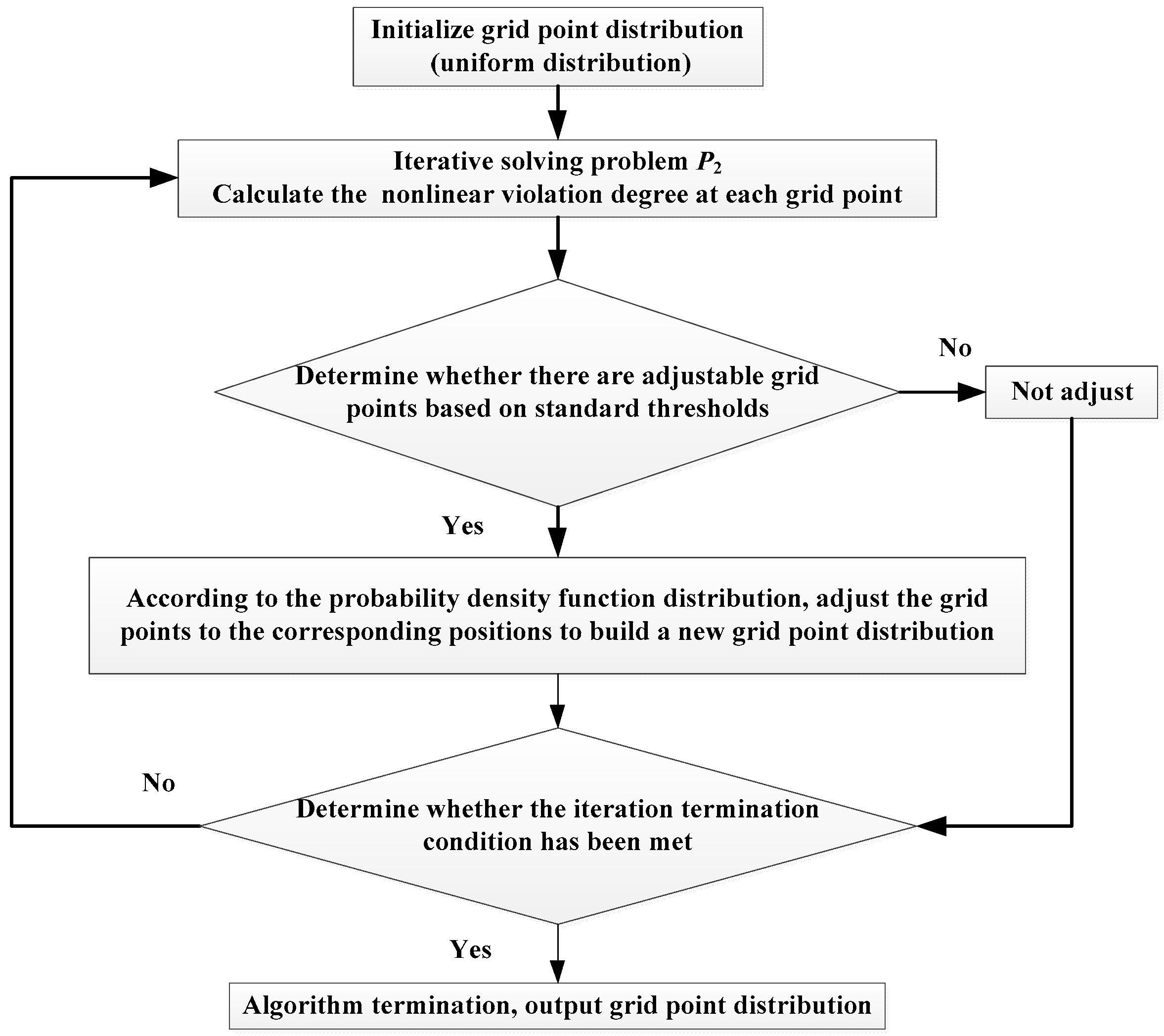
5. Grid Points’ Dynamic Adjustment Method Design

In the iterative solution process of convex optimization algorithms for problems, the iterative solution is represented in discrete form. A reasonable design of the grid points not only improves the convergence of the algorithm but also affects the approximate solution error of the optimization trajectory with the accuracy of each grid point [38]. The number of grid points solved in the k-th iteration is N, and the approximate solution error of the i-th grid point is defined as

$${\chi }_i={‖s^{(k)}\left(l_i\right)-{\overline{s}}^{(k)}\left(l_i\right)‖}_2$$

(42)

where $s^{(k)}$ represents the state vector of the k-th iteration solution; ${\overline{s}}^{(k)}$ represents the integral state vector without linearization error, expressed as

$${\overline{s}}^{(k)}\left(l_i\right)={\displaystyle {\int }_{l_i}^{l_{i+1}}\dot{s}\left(s,u,l\right)dl}$$

(43)

The adjustment function of the grid point is defined as follows:

$$F^{\prime }(l_i)=\left\{\begin{array}{ll}1\hfill & if i=0 or i=N\hfill \\ 0\hfill & if {\chi }_i\le {\chi }_{nord} (0<i<N)\hfill \\ {\chi }_i/{\chi }_{nord}\hfill & if {\chi }_i>{\chi }_{nord} (0<i<N)\hfill \end{array}\right.$$

(44)

where χ_nord represents the default threshold for the approximate solution error of the grid points. In this paper, the grid point positions at both ends are set to be fixed; therefore, their function values remain 1 throughout the iterative solution process. When the approximate solution error of the grid points is less than the default threshold, its function value is 0, indicating that the degree of non-linear violation of the grid points here is relatively small, and the position of the grid points here can be changed. The number of grid points, which need to be adjusted for each iteration solution, is the number of grid points where all function values are 0.

$$\Delta {\chi }^k=count(F^{\prime }(l_i)=0)$$

(45)

The probability density function of the adjusted grid point is defined as follows:

$$F(l_i)=F^{\prime }(l_i)/{\displaystyle \sum _{i=1}^{N^{k+1}}{F}^{\prime }(l_i)\Delta l_i}$$

(46)

According to Equation (46), the probability density of the grid points at any position in the lateral distance domain can be interpolated and calculated. Calculate the corresponding cumulative probability distribution function according to F(l_i), and select the position with a cumulative probability of j/(Δχ^k + 1), j = 1, …, Δχ^k as the corresponding newly added grid point position according to the number of grid points, which need to be adjusted.

Set the algorithm iteration termination conditions as follows:

$$\underset{1\le i\le N}{\max }\left|s^{(k+1)}\left(l_i\right)-s^{(k)}\left(l_i\right)\right|\le \epsilon$$

(47)

where ε is the algorithm convergence threshold, which is the same as the s dimension. The dynamic adjustment process of the grid points in the algorithm is shown in Figure 3.

6. Simulation Verification

6.1. Experimental Parameter Setting

It is assumed that the interceptor adopts a high throw re-entry glide trajectory mode, and this paper focuses on the trajectory of the interceptor in the midcourse guidance re-entry glide phase. The initial states are set to [h₀, z₀, x₀, v₀, θ₀, ψ_v0] = [7 × 10⁴/r_e, 0, 0, 3 × 10³/$\sqrt{g_0{r}_e}$, −5°, 0°]. The process constraints are limited to Q_max= 1 × 10⁶ J/(m²s), p_max = 1 × 10⁵ Pa, n_max = 8 g. The control variable constraints are limited to |α| ≤ 30°, |σ| ≤ 85°. The constraint radius of the trust region is set to [δ_h, δ_z, δ_x, δ_v, δ_θ, δ_ψv, δ_α, δ_σ] = [2 × 10⁴/r_e, 2 × 10³/r_e, 2 × 10³/r_e, 500/$\sqrt{g_0{r}_e}$, 20π/180, 30π/180, 10π/180, 90π/180]. The convergence thresholds are set to [ε_h, ε_z, ε_x, ε_v, ε_θ, ε_ψv, ε_α, ε_σ] = [200/re, 20/re, 20/re, 50/$\sqrt{g_0{r}_e}$, π/180, 5π/180, π/180, 5π/180]. The number of grid points in the iterative solution of the convex optimization algorithm is set to N = 200; the maximum number of iterations is 500; and the approximation solution error threshold is χ_nord = 1 × 10⁻⁶. This paper uses Python 3.10 to program the simulation experiments; MATLAB R2016a to plot the simulation data; and the ECOS-BB solver for convex sequence planning.

Set the parameters related to the DDPG algorithm as follows. The simulation step size is set to $\Delta t$ = 1/$\sqrt{r_e/g_0}$; the discount factor is set to 0.99; the maximum number of training sessions is set to 5 × 10⁴; the number of random training samples is set to 2 × 10³; and the capacity of the memory bank is set to 1 × 10⁶. The actor network adopts the 9-300-2 hierarchical structure; the critical network adopts the 11-300-2 hierarchical structure; the network parameter optimizer uses the Adam optimizer; and the network learning rate is set to 0.0001.

6.2. The Effectiveness of Initial Solution Trajectories’ Rapid Generation Method Verification

In order to verify the effectiveness of the rapid initial solution trajectory generation method based on the DDPG algorithm proposed, this paper evaluates the convergence of the DDPG algorithm training by observing the changes in average rewards; the specific meaning of average rewards can be found in Ref [30], and the average reward index is set to 800. Simultaneous selection of multiple terminal end positions ([$h_f^1$, $z_f^1$, $x_f^1$] = [3 × 10⁴/r_e, 0, 3.38 × 10⁵/r_e], [$h_f^2$, $z_f^2$, $x_f^2$] = [3 × 10⁴/r_e, 2.5 × 10⁴/r_e, 3.38 × 10⁵/r_e], [$h_f^3$, $z_f^3$, $x_f^3$] = [3 × 10⁴/r_e, −2.5 × 10⁴/r_e, 3.38 × 10⁵/r_e]) is performed for initial solution trajectory generation experiments. The simulation results are shown in Figure 4.

Figure 4a shows that the average reward of the DDPG algorithm shows an overall upward trend during the training process, and when the number of training iterations is 15,130, the average reward reaches the set training index, indicating that the DDPG algorithm can converge in the training of the initial solution generation task of the guidance trajectory. Figure 4b shows that the three initial solution trajectories generated by this method are not only relatively smooth but also meet the basic guidance requirements. In addition, the generation time of these three initial solution trajectories is 0.15 s, 0.14 s, and 0.15 s, all of which meet the time requirements for rapid trajectory generation.

6.3. The Superiority of Initial Solution Trajectories’ Rapid Generation Method Verification

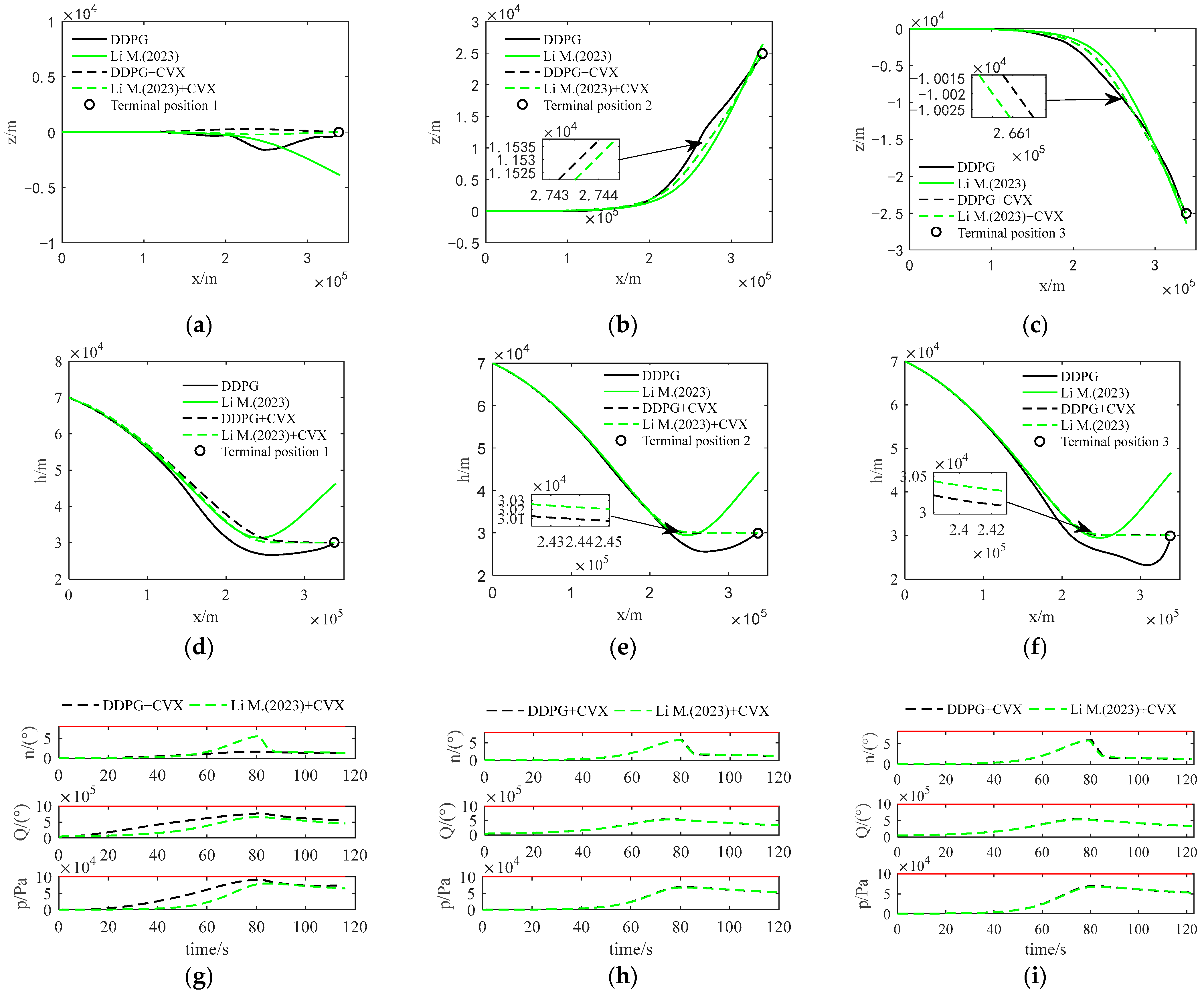
In order to verify the superior performance of the trajectory convex optimization algorithm with the trajectories generated by the DDPG algorithm as the initial solution in this paper, three terminal end positions are used as three scenarios in Section 6.2, and a simulation comparison experiment is conducted using the initial solution trajectory generation algorithm from Ref [38]. The grid point strategies for both algorithms are uniformly distributed, and the simulation results are shown in Figure 5.

In Figure 5, DDPG represents the initial solution trajectory curve obtained using the DDPG algorithm; Li M. (2023) represents the initial solution trajectory curve obtained using the initial solution trajectory generation algorithm from Ref [38]; DDPG + CVX refers to the optimized trajectory curve obtained via convex optimization of the trajectory based on the initial solution trajectory solved using the DDPG algorithm; and Li M. (2023) + CVX represents the optimized trajectory curve obtained via convex optimization of the trajectory based on the initial solution trajectory generated by the algorithm from Ref [38].

As shown in Figure 5, the optimal trajectories obtained by the two convex optimization methods are very similar, but the guiding effect of the initial solution generated by the DDPG algorithm is significantly better than that of the method from Ref [31] in all three scenarios (see Figure 5a–f). Moreover, the optimal trajectories in all three scenarios can satisfy the process constraints (see Figure 5g–i), indicating that the trajectory planned by the improved convex optimization algorithm in this paper is effective.

To effectively assess the comparative advantages and disadvantages of the two methods, this article randomly selects terminal positions and subsequently carries out 100 Monte Carlo simulations utilizing both approaches. Each simulation’s resulting data are recorded. Ultimately, the statistical averages of these data are computed and utilized for comparison, as shown in

Table 1. Comparison of simulation data between DDPG + CVX and Li M. (2023) + CVX methods.

Method	DDPG + CVX	Li M.(2023) + CVX
Iterations	5.27	6.31
CPU Time [s]	30.9623	36.8741
Objective Function Value	0.2144	0.2193
Terminal Position Errors [m]	0.5388	2.3413

.

As is evident in Table 1, in Monte Carlo simulations, the DDPG + CVX algorithm in this paper necessitates less iteration to attain an optimized trajectory compared to the convex optimization method from Ref [31]. Furthermore, the corresponding solving time is reduced by approximately one-fifth, on average. Notably, despite achieving similar objective function value, the average terminal position error generated by the DDPG + CVX algorithm is smaller than that of the convex optimization method from Ref [31]. This is attributed to the fact that the initial trajectory generated by the DDPG approach in this article exhibits a higher degree of accuracy. Consequently, this serves as a beneficial prerequisite for the convex optimization algorithm, enabling it to swiftly and precisely converge to the optimal trajectory during iterative solving.

The simulation results show that the improved convex optimization algorithm proposed in this paper improves the efficiency and accuracy of solving the trajectory planning problem in the midcourse guidance phase.

6.4. The Effectiveness of Grid Point Dynamic Adjustment Method Verification

In order to verify the effectiveness of the dynamic adjustment method for grid points based on the distribution of approximate solution errors designed in this paper, a simulation comparison analysis with the traditional uniform grid point distribution method was performed using Scenario 2 in Section 6.3 as an example. The simulation results are shown in Figure 6. The approximate solution error of the trajectory is defined as the integration difference between the optimized trajectory and the actual trajectory [32].

As shown in Figure 6, the iterative longitudinal trajectory of both methods can quickly converge to the optimal trajectory (see Figure 6a,d), but the iterative lateral trajectory of the traditional method is obviously not as good as that of the improved method (see Figure 6b,e). Compared with traditional methods, the improved method only requires four iterations, and in the final grid point distribution of the improved method, the grid points at both ends of the trajectory are relatively sparse, while the grid points in the middle are relatively dense (see Figure 6c,f). This is because the trajectory turns laterally in the middle stage, increasing the demand for overload, and the non-linearity of this part of the trajectory is relatively high. Therefore, the improved method’s grid point adjustment strategy allocates more grid points in the middle stage of the trajectory.

Similar to Section 6.3, to effectively assess the comparative advantages and disadvantages of the two methods, this article randomly selects terminal positions and subsequently carries out 100 Monte Carlo simulations utilizing both approaches. Each simulation’s resulting data are recorded. Ultimately, the statistical averages of these data are computed and utilized for comparison, as shown in

Table 2. Comparison of simulation data between improved and traditional methods.

Method	Improved	Traditional
Iterations	4.36	5.25
CPU Time [s]	25.3326	32.0201
Objective Function Value	0.2141	0.2182
Approximate Solution Error	0.0186	0.0327

.

As shown in Table 2, the improved method is better than traditional methods in terms of iterations and CPU time. Although the objective function values obtained by the two methods are similar, the approximate solution error of the trajectory obtained by the improved method is reduced by about half compared to the traditional method. This is because the improved method gradually distributes more grid point positions in areas with higher non-linearity during the iterative solution process under the designed grid point dynamic adjustment method (such as Equations (42)–(46)), reducing the degree of non-linearity violation of the trajectory and thus reducing the approximate solution error of the obtained trajectory.

The simulation results show that the designed grid point dynamic adjustment method based on the approximation error distribution not only improves the optimization efficiency of the convex optimization algorithm but also greatly reduces the approximation error of the optimized trajectory, making it more conducive to the subsequent trajectory tracking processing.

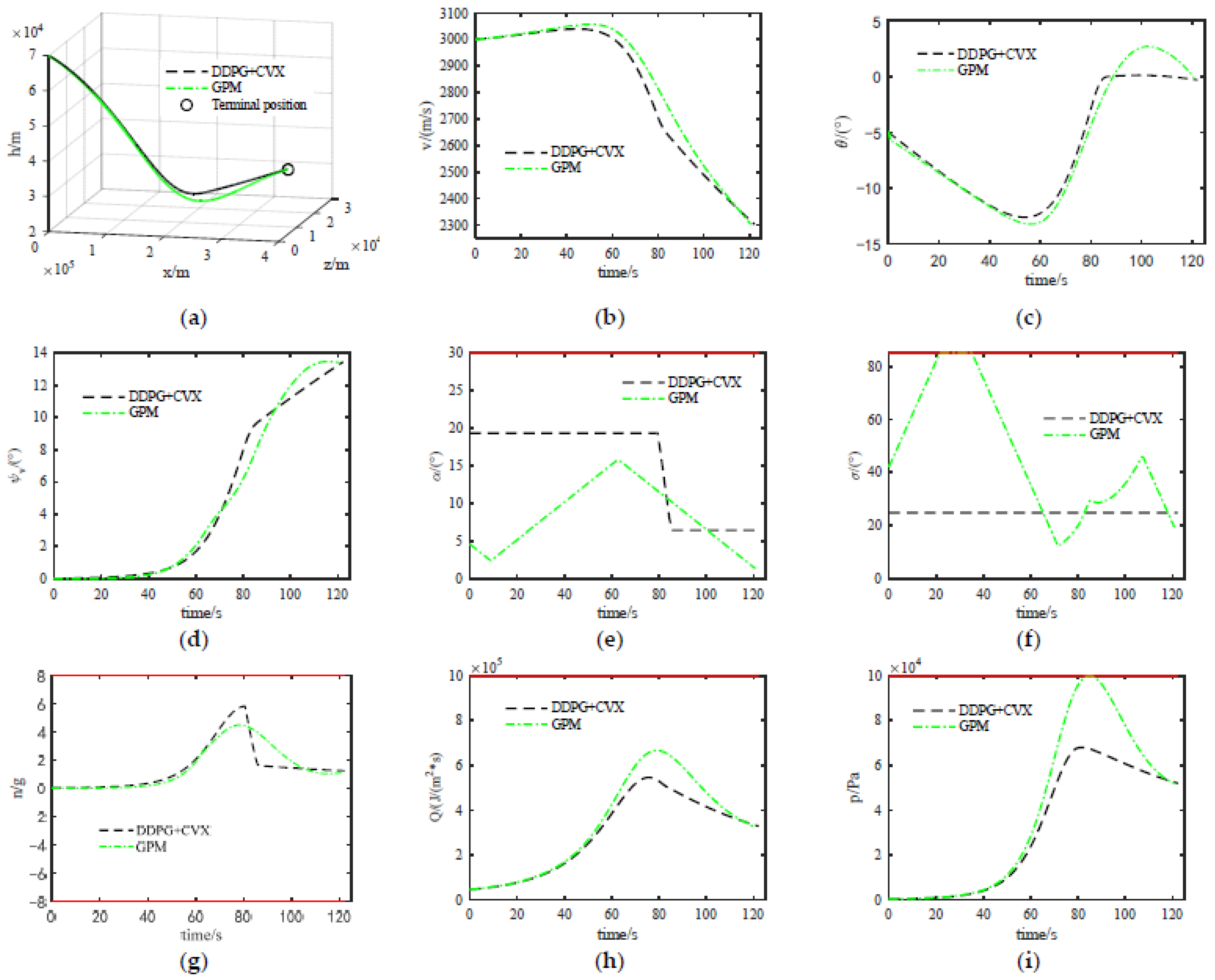
6.5. The Performance of Improved Convex Optimization Method Verification

In order to verify the optimization performance and the ability to meet the constraints of the method proposed in this paper, a simulation comparison analysis with the Gauss pseudospectral method (GPM) was performed using Scenario 2 in Section 6.3 as an example. The simulation results are shown in Figure 7 and

Table 3. Data parameters of two methods.

Method	Flight Time of Optimized Trajectory [s]	CPU Time [s]	Objective Function Value
DDPG + CVX	122.2778	24.5023	0.2143
GPM	120.7305	63.5632	0.2106

.

In Figure 7, GPM represents the Gauss pseudospectral method.

As shown in Figure 7, the optimized trajectories of the two methods can meet the guidance requirements, and the trajectories are smooth (see Figure 7a), with relatively stable changes in their respective state variables (see Figure 7b–d). The changes in the angle of attack and pitch angle of the optimized trajectory using the DDPG + CVX method are significantly smaller than those of the GPM method (see Figure 7e,f), indicating that the DDPG + CVX method is more conducive to the tracking and control of subsequent trajectories. In addition, the optimized trajectories of the two methods can meet the requirements of process constraints (see Figure 7g,i). As can be seen in Table 3, the trajectory optimization accuracy of the GPM method is slightly higher, but the optimization accuracies of the two methods are not much different, and the optimization time and approximate solution error of the DDPG + CVX method are much smaller than those of the GPM method. Therefore, the comparison of the simulation data between the two methods shows that the optimization performance of the two methods is approximately the same, and both can meet the constraints in the guidance process. However, the optimization efficiency of the DDPG + CVX method is significantly better.

7. Conclusions

The aim of this paper is to improve the efficiency and accuracy of convex optimization algorithms in dealing with the problem of midcourse guidance trajectory planning for an interceptor. The main conclusions are as follows: (1) Propose the concept of lateral distance domain, transform the motion model from time domain to lateral distance domain, and establish the discrete trajectory convex optimization model in the lateral distance domain; (2) Design the corresponding MDP based on the characteristics of the midcourse guidance trajectory planning model, and propose the fast initial solution trajectory generation method based on the DDPG algorithm; (3) Use the concept of probability density function, and design the dynamic adjustment method of grid points based on the distribution of approximate solution error. The simulation experimental data show that the improved trajectory convex programming algorithm proposed in this paper improves the solving efficiency and optimization accuracy of the algorithm, reducing the approximate solution error of the optimized trajectory.

In addition, in the context of the rapid development of big data technology, data-driven trajectory planning is a promising research direction, which also makes the deep reinforcement learning algorithm—which can realize this technology—have broad application prospects in trajectory planning. The research content of this article verifies the feasibility of its application, and future research will be conducted to extend it to more complex scenarios.

References

- Carbone, A.; Grossi, D.; Spiller, D. Cutting-edge trajectory optimization through quantum annealing. Appl. Sci. 2023, 13, 12853. [Google Scholar] [CrossRef]
- Cheng, L.; Shi, P.; Gong, S.; Wang, Z. Real-time trajectory optimization for powered planetary landings based on analytical shooting equations. Chin. J. Aeronaut. 2022, 35, 91–99. [Google Scholar] [CrossRef]
- Grant, M.; Braun, R. Rapid indirect trajectory optimization for conceptual design of hypersonic missions. J. Spacecr. Rocket. 2015, 52, 177–182. [Google Scholar] [CrossRef]
- Shen, H.; Casalino, L.; Luo, Y. Global search capabilities of indirect methods for impulsive transfers. J. Astronaut. Sci. 2015, 62, 212–232. [Google Scholar] [CrossRef]
- Lee, D.; Bang, H.; Kim, H. Optimal earth-moon trajectory design using new initial costate estimation method. J. Guid. Control Dyn. 2012, 35, 1671–1676. [Google Scholar] [CrossRef]
- Ren, F.; Li, R.; Xu, J.; Feng, C. Indirect optimization for finite thrust orbit transfer and cooperative rendezvous using an initial guess generator. Adv. Space Res. 2023, 71, 2575–2590. [Google Scholar] [CrossRef]
- Hur, S.; Lee, S.; Nam, Y.; Kim, C. Direct dynamic- simulation approach to trajectory optimization. Chin. J. Aeronaut. 2021, 34, 6–19. [Google Scholar] [CrossRef]
- Peng, H.; Wang, X.; Li, M.; Chen, B. An hp symplectic pseudospectral method for nonlinear optimal control. Commun. Nonlinear Sci. Numer. Simul. 2017, 42, 623–644. [Google Scholar] [CrossRef]
- He, S.; Hu, C.; Lin, S.; Zhu, Y.; Tomizuka, M. Real-time time-optimal continuous multi-axis trajectory planning using the trajectory index coordination method. ISA Trans. 2022, 131, 639–649. [Google Scholar] [CrossRef]
- Malyuta, D.; Reynolds, T.; Szmuk, M.; Mesbahi, M.; Açıkmese, B.; Carson, J., III. Discretization performance and accuracy analysis for the powered descent guidance problem. In Proceedings of the AIAA SCITECH 2019 Forum, San Diego, CA, USA, 7–11 January 2019. [Google Scholar]
- Guo, X.; Zhu, M. Direct trajectory optimization based on a mapped Chebyshev pseudospectral method. Chin. J. Aeronaut. 2013, 26, 401–412. [Google Scholar] [CrossRef]
- Guang, Z.; Bi, X.; Bin, L. Optimal deployment of spin-stabilized tethered formations with continuous thrusters. Nonlinear Dyn. 2019, 95, 2143–2162. [Google Scholar] [CrossRef]
- Zhang, L.; Gao, H.; Chen, Z.; Sun, Q.; Zhang, X. Multi-objective global optimal parafoil homing trajectory optimization via Gauss pseudospectral method. Nonlinear Dyn. 2013, 72, 1–8. [Google Scholar] [CrossRef]
- Zhang, C.; Zhu, Y.; Yang, L.; Zeng, X.; Zhang, R. Numerical solution for elliptical orbit pursuit-evasion game via deep neural networks and pseudospectral method. Proc. Inst. Mech. Eng. Part G J. Aerosp. Eng. 2023, 237, 796–808. [Google Scholar] [CrossRef]
- Li, Y.; Chen, W.; Zhou, H.; Yang, L. Conjugate gradient method with pseudospectral collocation scheme for optimal rocket landing guidance. Aerosp. Sci. Technol. 2020, 104, 105999. [Google Scholar] [CrossRef]
- Azar, A.; Koubaa, A.; Ali, M.; Ibrahim, H.; Ibrahim, Z.; Kazim, M.; Ammar, A.; Benjdira, B.; Khamis, A.; Hameed, I.; et al. Drone deep reinforcement learning: A review. Electronics 2021, 10, 999. [Google Scholar] [CrossRef]
- Pan, Y.; Boutselis, G.; Theodorou, E. Efficient Reinforcement Learning via Probabilistic Trajectory Optimization. IEEE Trans. Neural Netw. Learn. Syst. 2018, 29, 5459–5474. [Google Scholar] [CrossRef] [PubMed]
- Zhao, J.; Zhou, R. Pigeon-inspired optimization applied to constrained gliding trajectories. Nonlinear Dyn. 2015, 82, 1781–1795. [Google Scholar] [CrossRef]
- Duan, H.; Li, S. Artificial bee colony-based direct collocation for reentry trajectory optimization of hypersonic vehicle. IEEE Trans. Aerosp. Electron. Syst. 2015, 51, 615–626. [Google Scholar] [CrossRef]
- Zhou, H.; Wang, X.; Cui, N. Glide trajectory optimization for hypersonic vehicles via dynamic pressure control. Acta Astronaut. 2019, 164, 376–386. [Google Scholar] [CrossRef]
- Li, Z.; Hu, C.; Ding, C.; Liu, G.; He, B. Stochastic gradient particle swarm optimization based entry trajectory rapid planning for hypersonic glide vehicles. Aerosp. Sci. Technol. 2018, 76, 176–186. [Google Scholar] [CrossRef]
- Gaudet, B.; Furfaro, R. Terminal adaptive guidance for autonomous hypersonic strike weapons via reinforcement metalearning. J. Spacecr. Rocket. 2023, 60, 286–298. [Google Scholar] [CrossRef]
- D’Ambrosio, A.; Furfaro, R. Learning fuel-optimal trajectories for space applications via Pontryagin neural networks. Aerospace 2024, 11, 228. [Google Scholar] [CrossRef]
- Malyuta, D.; Yu, Y.; Elango, P.; Açıkmeşe, B. Advances in trajectory optimization for space vehicle control. Annu. Rev. Control 2021, 52, 282–315. [Google Scholar] [CrossRef]
- Nicholas, O.; David, K.; Aaron, A. Autonomous optimal trajectory planning for orbital rendezvous, satellite inspection, and final approach based on convex optimization. J. Astronaut. Sci. 2021, 68, 444–479. [Google Scholar]
- Sagliano, M.; Seelbinder, D.; Theil, S.; Lu, P. Six-degree-of-freedom rocket landing optimization via augmented convex-concave decomposition. J. Guid. Control Dyn. 2024, 47, 20–35. [Google Scholar] [CrossRef]
- Wang, Z.; Grant, M. Constrained trajectory optimization for planetary entry via sequential convex programming. J. Guid. Control Dyn. 2017, 40, 2603–2615. [Google Scholar] [CrossRef]
- Liu, X.; Shen, Z.; Lu, P. Exact convex relaxation for optimal flight of aerodynamically controlled missiles. IEEE Trans. Aerosp. Electron. Syst. 2016, 52, 1881–1892. [Google Scholar] [CrossRef]
- Cheng, X.; Li, H.; Zhang, R. Efficient ascent trajectory optimization using convex models based on the Newton–Kantorovich/Pseudospectral approach. Aerosp. Sci. Technol. 2017, 66, 140–151. [Google Scholar] [CrossRef]
- Bae, J.; Lee, S.; Kim, Y.L.; Kim, S. Convex optimization-based entry guidance for spaceplane. Int. J. Control Autom. 2022, 20, 1652–1670. [Google Scholar] [CrossRef]
- Zhou, X.; He, R.; Zhang, H.; Tang, G.; Bao, W. Sequential convex programming method using adaptive mesh refinement for entry trajectory planning problem. Aerosp. Sci. Technol. 2021, 109, 106374. [Google Scholar] [CrossRef]
- Sagliano, M. Pseudospectral convex optimization for powered descent and landing. J. Guid. Control Dyn. 2018, 41, 320–334. [Google Scholar] [CrossRef]
- Sagliano, M. Generalized hp Pseudospectral-Convex Programming for Powered Descent and Landing. J. Guid. Control Dyn. 2019, 42, 1562–1570. [Google Scholar] [CrossRef]
- Sagliano, M.; Heidecker, A.; Macés, H.; Farì, S.; Schlotterer, M.; Woicke, S.; Seelbinder, D.; Dumont, E. Onboard guidance for reusable rockets: Aerodynamic descent and powered landing. In Proceedings of the AIAA Scitech 2021 Forum, Online, 11–15 January 2021. [Google Scholar]
- Sagliano, M.; Mooij, E. Optimal drag-energy entry guidance via pseudospectral convex optimization. Aerosp. Sci. Technol. 2021, 117, 106946. [Google Scholar] [CrossRef]
- Song, Y.; Miao, X.; Gong, S. Adaptive powered descent guidance based on multi-phase pseudospectral convex optimization. Acta Astronaut. 2021, 180, 386–397. [Google Scholar] [CrossRef]
- Li, W.; Li, J.; Li, N.; Shao, L.; Li, M. Online trajectory planning method for midcourse guidance phase based on deep reinforcement learning. Aerospace 2023, 10, 441. [Google Scholar] [CrossRef]
- Li, M.; Zhou, C.; Shao, L.; Lei, H.; Luo, C. A trajectory generation algorithm for a re-entry gliding vehicle based on convex optimization in the flight range domain and distributed grid Points adjustment. Appl. Sci. 2023, 13, 1988. [Google Scholar] [CrossRef]
Figure 1.
Trajectory planning concept in the lateral distance domain.
Figure 2.
Trajectory planning task training framework.
Figure 3.
Grid point dynamic adjustment process.
Figure 4.
Algorithm validation effect chart: (a) DDPG algorithm training convergence curve; (b) Initial solution trajectory curve.
Figure 5.
Comparison of optimization trajectories between two methods: (a) Lateral trajectory of Scenario 1; (b) Lateral trajectory of Scenario 2; (c) Lateral trajectory of Scenario 3; (d) Vertical trajectory of Scenario 1; (e) Vertical trajectory of Scenario 2; (f) Vertical trajectory of Scenario 3; (g) Constraint curve of Scenario 1; (h) Constraint curve of Scenario 2; (i) Constraint curve of Scenario 3.
Figure 6.
Comparison of simulation results between two methods: (a) Improved lateral trajectory; (b) Improved vertical trajectory; (c) Improved grid point iteration; (d) Traditional lateral trajectory; (e) Traditional vertical trajectory; (f) Traditional grid point iteration.
Figure 7.
Comparison of simulation results between two methods: (a) Trajectory; (b) Speed; (c) Trajectory inclination angle; (d) Trajectory deflection angle; (e) Angle of attack; (f) Angle of bank; (g) Overload; (h) Heat flow density; (i) Dynamic pressure.