Aerodynamic Analysis of Deorbit Drag Sail for CubeSat Using DSMC Method

Abstract

Reducing space debris is a critical challenge in current space exploration. This study focuses on designing a drag sail for CubeSat models and examining their aerodynamic properties using the direct simulation Monte Carlo (DSMC) method. The analysis encompasses the aerodynamic performance of intricate three-dimensional shapes with varying sail dimensions at orbital altitudes of 125 km, 185 km, 300 km, and 450 km. Additionally, free molecular flow (FMF) theory is applied and compared with the DSMC findings for both a flat-plate model and the CubeSat. The results reveal that FMF accurately predicts the drag coefficient at altitudes of 185 km and above, while significant discrepancies occur at lower altitudes due to increased inter-molecular collisions. This study also suggests that the drag sail substantially enhances the CubeSat’s drag force, which effectively reduces its deorbiting time.

1. Introduction

CubeSats are a type of satellite with standardized sizes in U (1 U = 10 cm × 10 cm × 10 cm) [1]. Such satellites are low-cost and have short development cycles, rendering them a popular choice for low-budget users [1,2]. Due to these features, CubeSats are extensively launched into orbit, further overcrowding orbit resources [3,4]. CubeSats in Low-Earth Orbit (LEO) gradually decrease in altitude owing to the rarefied aerodynamic drag until re-entry [5]. This process takes decades and can occupy the limited orbit resources. CubeSats will become pieces of debris unless proper end-of-life disposal is performed [6]. It is an urgent task for engineers to limit the rapid growth of space debris caused by space activities to avoid potential future risks [7,8,9]. In order to boost the deorbiting process of the CubeSat, four kinds of deorbiting equipment are available: electrodynamic force tethers [10], onboard thrusters [11], solar radiation pressure sails [12], and aerodynamic drag sails [13].

A drag sail is light, simple in structure, and reliable to deploy [14]. It has become a hot topic for researchers in recent years, and extensive theoretical and experimental studies can be found in the literature [15,16]. Poland’s PW-Sat2 [17] was launched in 2018 and deployed the drag sail successfully. PW-Sat2 was 2U and aimed to test the structure and mechanism design of the sail and forecast the deorbiting time. However, the sail was damaged due to the sharp change in thermal conditions. AEOLDOS [18] is a deorbit module proposed by researchers from the UK and Germany to study the folding pattern and deployment process in detail. CanX-7 [19] is a Canadian demonstration mission for a drag sail device, and the study discussed the design of the configuration, structure, and electrical architecture. Nikolajsen and Kristensen [20] studied the folding and thermal performance of the drag sail. These previous studies have already given detailed examples of sail structure and mechanism design. However, the optimization of the sail size of a CubeSat has received little attention, and the drag coefficient ($C_D$) was generally set to a constant value based on FMF in previous studies [21,22]. As the altitude decreases, FMF will no longer provide correct results, and the DSMC method is a more reliable tool that has already demonstrated its capabilities in rarefied gas dynamics [23].

The purpose of this study is to focus on the aerodynamic characteristics of a CubeSat before and after deploying a drag sail. The design and assessment of such a drag sail are presented in detail. This work also tested the effectiveness of FMF for different altitudes and flow regimes. The structure of the paper is as follows: Section 2 introduces basic information about the CubeSat and the design of the drag sail. Section 3 discusses the analytical and numerical methods used in this study to present flow simulations and orbit forecasts, as well as the corresponding validation cases. Section 4 demonstrates the simulation works in detail and compares the results obtained by different methods. The reason for the relative error is also analyzed. Section 5 presents the orbital decay forecast of the CubeSat with and without the drag sail based on the data computed in previous sections. The forecast result demonstrates the high deorbiting efficiency of the drag sail.

2. The Design of the Drag Sail

MOVE-III is proposed to be the fourth CubeSat of the Munich Orbital Verification Experiment (MOVE), a student project at the Technical University of Munich [24]. The CubeSat has a size of 6U and carries scientific payloads to perform in situ observations [25] of sub-millimeter space debris and meteoroids in LEO based on the Munich Dust Counter [26]. MOVE-III is a typical CubeSat suitable for mounting a deorbit drag sail to fulfill its end-of-life disposal. A detailed CAD assembly model of MOVE-III is available in this study for further simplification (see Figure 1). The configuration of MOVE-III has three main parts: a deployable antenna, deployable solar panels, and the body frame [24]. Since MOVE-III is a CubeSat for scientific experiments and research, the total volume reserved for the drag sail system is assumed to be 1 U.

Theoretically, the drag sail can assume any axially symmetric shape to prevent additional pitch and yaw moments, and if the shape is centrally symmetric, the internal stresses can be evenly distributed to each beam. However, the total mass of the structure increases and the reliability and stability of the system decrease as the number of edges and vertices of the sail increases. Hence, a square sail was selected for analysis in MOVE-III.

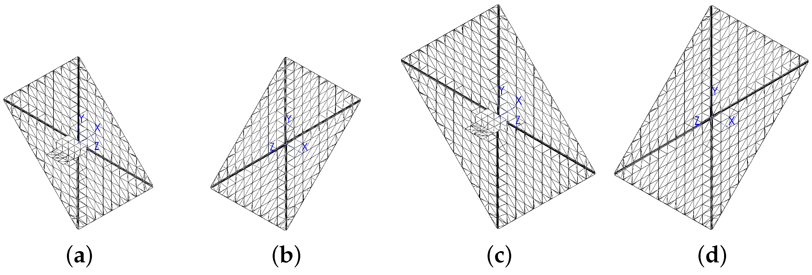
ADE is a 1U CubeSat designed by Purdue University and is equipped with a drag sail with a 1.346 m² cross-sectional area [27]. The NUST-3 CubeSat reserves 1.5 U onboard space for a 7.84 m² sail. By taking these previous drag sail designs as references, this study will discuss two alternative sail configurations with areas of 4 m² and 6.25 m² (see Figure 2).

3. Methodology and Code Validation

The orbital altitudes of interest in this work cover the transitional and free molecular flow regimes (see Section 4.1). The rarefaction of a flow is described by a dimensionless parameter, the Knudsen number [23], $Kn=\lambda /L$, where $\lambda$ is the mean free path, and L is the characteristic length. Free molecular flow (FMF) satisfies $Kn\ge 10$, while transitional flow satisfies $0.1\le$ $Kn<10$ [28].

The direct simulation Monte Carlo (DSMC) method directly generates simulated particles to represent real particles and enables collisions between simulated particle pairs to be modeled with the same physical considerations as real molecular pairs [23]. The results of the simulation are averaged at each time step to obtain macroscopic steady-state values, including velocity, temperature, pressure, force, etc. Therefore, DSMC is a statistical numerical approach. Nowadays, the method is widely applied to the analysis of re-entry spacecraft [29,30] and LEO satellites [31] and is favored by researchers and engineers [21,27]. SPARTA is an open-source DSMC computational kernel for the simulation of rarefied gas flows using collision, chemistry, and boundary condition models [32]. It is capable of performing simulations of low-density gases in 2D or 3D. Particles are tracked and grouped through a Cartesian grid that overlays the simulation box. Physical objects with line segments in 2D or triangulated surfaces in 3D can be embedded in the grid.

Before simulating 3D cases with SPARTA, it is a conventional prerequisite to check its installation and performance by replicating a previous study; in this case, the ADE from Purdue University was used [27]. By setting the SPARTA input parameters to the same values in the literature, $C_D$ at a 185 km orbital altitude and zero incident angles ($\alpha$ = 0, $\beta$ = 0) is found to be identical to the reference value.

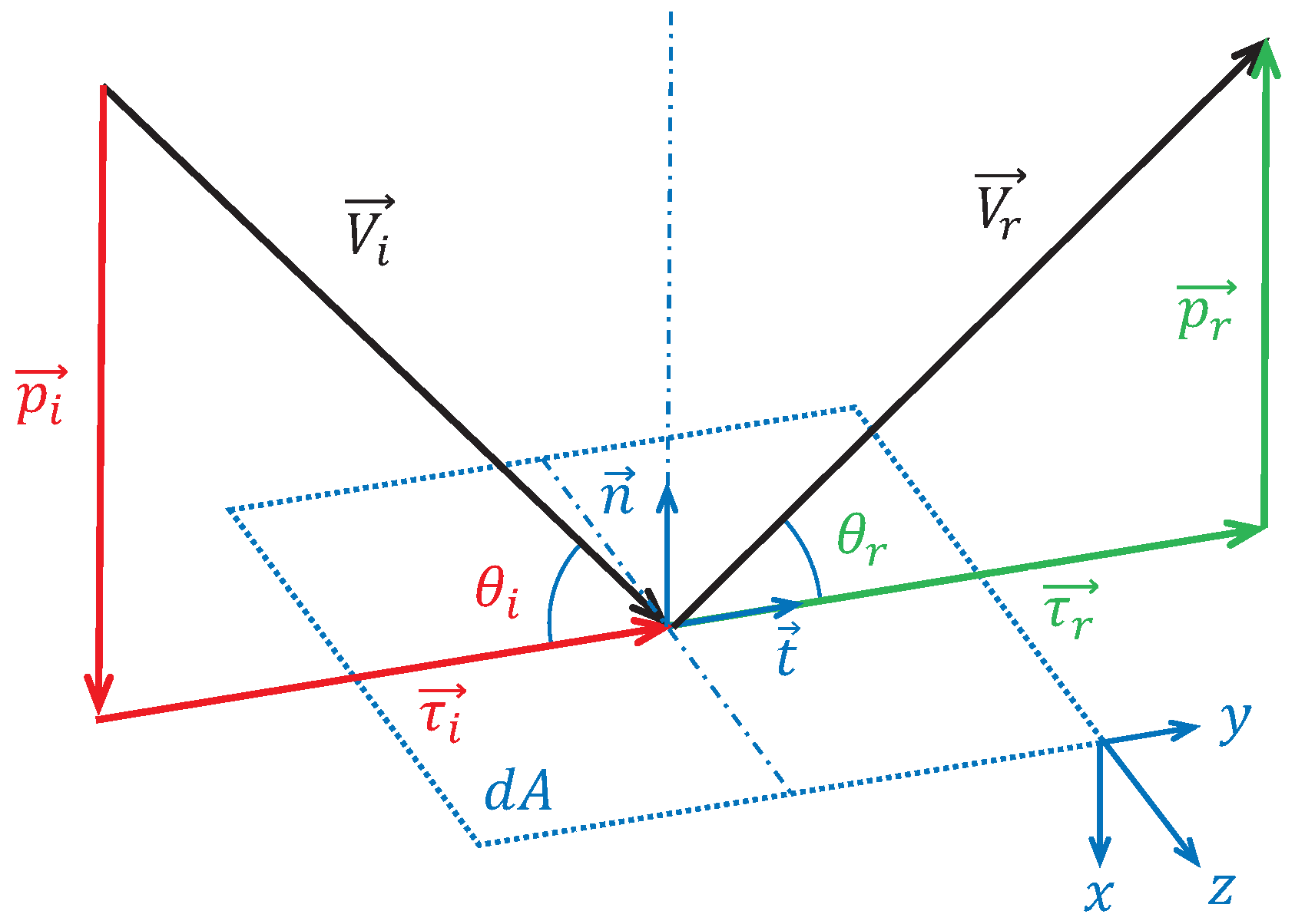
Gas–surface interaction (GSI) is the main feature of FMF, where collisions between molecules are rare [33]. Incident particles neither collide with each other nor are influenced by reflected particles. Figure 3 is a schematic of this process based on the devised panel method. GSI is governed by the momentum relation [21]:

$$\frac{d\overrightarrow{f}}{dA}=(p_i+p_r)\overrightarrow{n}+({\tau }_i-{\tau }_r)\overrightarrow{t}$$

(1)

where $\frac{d\overrightarrow{f}}{dA}$ is the force acting on a surface element, $p_i$ and $p_r$ are the normal stresses of incident and reflection particles on the surface element, ${\tau }_i$ and ${\tau }_r$ are the shear stresses, respectively, $\overrightarrow{n}$ is the surface inward normal vector, and $\overrightarrow{t}$ is the local velocity direction tangential vector.

A flat plate with a characteristic length of 1 m was used for the validation of the FMF theory in calculating $C_D$ [31]. The result (see Figure 4) indicates that FMF fits the DSMC result well for altitudes higher than or equal to 170 km due to the increasing rarefaction of the atmosphere.

4. Aerodynamic Analysis of MOVE-III

The aerodynamic characteristic analysis of MOVE-III involves two configurations: before and after the deployment of the sail. Both DSMC and FMF were employed in this analysis, and an assessment was conducted to compare their agreement. The suitability of FMF in predicting the aerodynamic effect under LEO conditions was also evaluated.

4.1. Numerical Setup

To evaluate the impact of the drag sail on the aerodynamic characteristics of the CubeSat, it is imperative to construct computational models of two corresponding MOVE-III configurations, namely, pre- and post-sail-deployment.

For pre-sail-deployment scenarios, MOVE-III exhibits an identical configuration to that used when conducting scientific endeavors in orbit. Nevertheless, the actual complete assembly is too intricate to be incorporated into the SPARTA kernel of the DSMC method. As a result, the assembly needs to be simplified (see Figure 1 in Section 2). In this study, the surface details of the CubeSat are disregarded, while substantial elements, such as the deployable antenna and solar panel, are preserved. The panel construction of the CubeSat without a sail is shown in Figure 5.

The main frame of MOVE-III has a size of 6U. Prior to its launch into orbit, the CubeSat was housed within the rocket’s payload adapter, and this configuration is referred to as the launch envelope, which denotes the size of MOVE-III’s frame. Once fully deployed in orbit, the movable components are extended to form the orbit envelope [24].

In the case of post-sail-deployment scenarios, the scale of the characteristic length is determined by the span of the sail. Consequently, the body structure can be simplified to flat boxes. In the simulation cases presented in this study, the thickness of the sail has a negligible impact on the results. Therefore, to avoid introducing multi-dimensional issues and to ensure the fitness of the mesh, a sail thickness of 1 mm is assumed. It should be noted that the asymmetry stemming from the deployed solar panel is also taken into account. Panel constructions of the CubeSat with both sail sizes are shown in Figure 6.

The dimensions of MOVE-III before and after sail deployment are shown in

Table 1. Dimensions of MOVE-III with and without deployed drag sail.

Parameter	Without Drag Sail		With Deployed Sail
	Launch	Orbit	4 m2 Case	6.25 m2 Case
$L_x$ [mm]	227	426.65	463.52	463.52
$L_y$ [mm]	109	520.74	2863.39	3570.50
$L_z$ [mm]	366	366	2863.39	3570.50
$N_{vertex}$	-	1052	1148	1556
$N_{panel}$	-	2112	2324	3140

. Note that $L_x$, $L_y$, and $L_z$ are the x-, y-, and z-dimensions, respectively; $N_{vertex}$ is the number of vertices; and $N_{panel}$ is the number of panels.

At the orbital altitudes of interest, free-stream velocities are assumed to be the perfect-circle orbital velocity (see

Table 2. Free-stream physical parameter settings.

Parameter	Value
Altitude [km]	125	185	300	450
Mean free path [m]	5.35	173	2595	3.46 × 104
Free-stream velocity [m/s]	7833	7797	7730	7644
Static temperature [K]	413	680	976	996
Density [kg/m3]	1.23 × 10−8	3.86 × 10−10	1.92 × 10−11	1.59 × 10−12
Number density [m−3]	2.86 × 1017	1.06 × 1016	6.51 × 1014	6.14 × 1013
Molar fraction of $N_2$	0.712	0.464	0.149	0.017
Molar fraction of $O_2$	0.085	0.031	0.006	0
Molar fraction of O	0.203	0.505	0.845	0.983

), $\sqrt{\frac{GM}{R+h}}$, where $G=6.674\times {10}^{-11}(\mathrm{N}·{\mathrm{m}}^2)/{\mathrm{kg}}^2$ is the gravitational constant, $M=5.972\times {10}^{24}\mathrm{kg}$ is the mass of the Earth, $R=6.371\times {10}^6\mathrm{m}$ is the average radius of the Earth, and h is the orbital altitude. Static temperatures, densities, number densities, and compositions of the incident flow are taken from the US Standard Atmosphere (1976) [34]. The GSI condition is assumed to be 100% diffuse.

To examine the effect of attitude on $C_D$, this study sets the angle of attack $\alpha$ and angle of sideslip $\beta$ to 0, 30, and 60 degrees. Thus, a total of nine attitudes are produced and labeled in

Table 3. Cases with different attitude numbers to be simulated.

Angle [deg]	$\mathit{\beta }=0$	$\mathit{\beta }=30$	$\mathit{\beta }=60$
$\alpha =0$	Case 00	Case 03	Case 06
$\alpha =30$	Case 30	Case 33	Case 36
$\alpha =60$	Case 60	Case 63	Case 66

. A case number consists of two digits. The former indicates $\alpha$, and the latter indicates $\beta$. The digits 0, 3, and 6 represent 0, 30, and 60 degrees, respectively. In this study, the surfaces of the test component are kept fixed, while free streams flow in with varying velocity vectors.

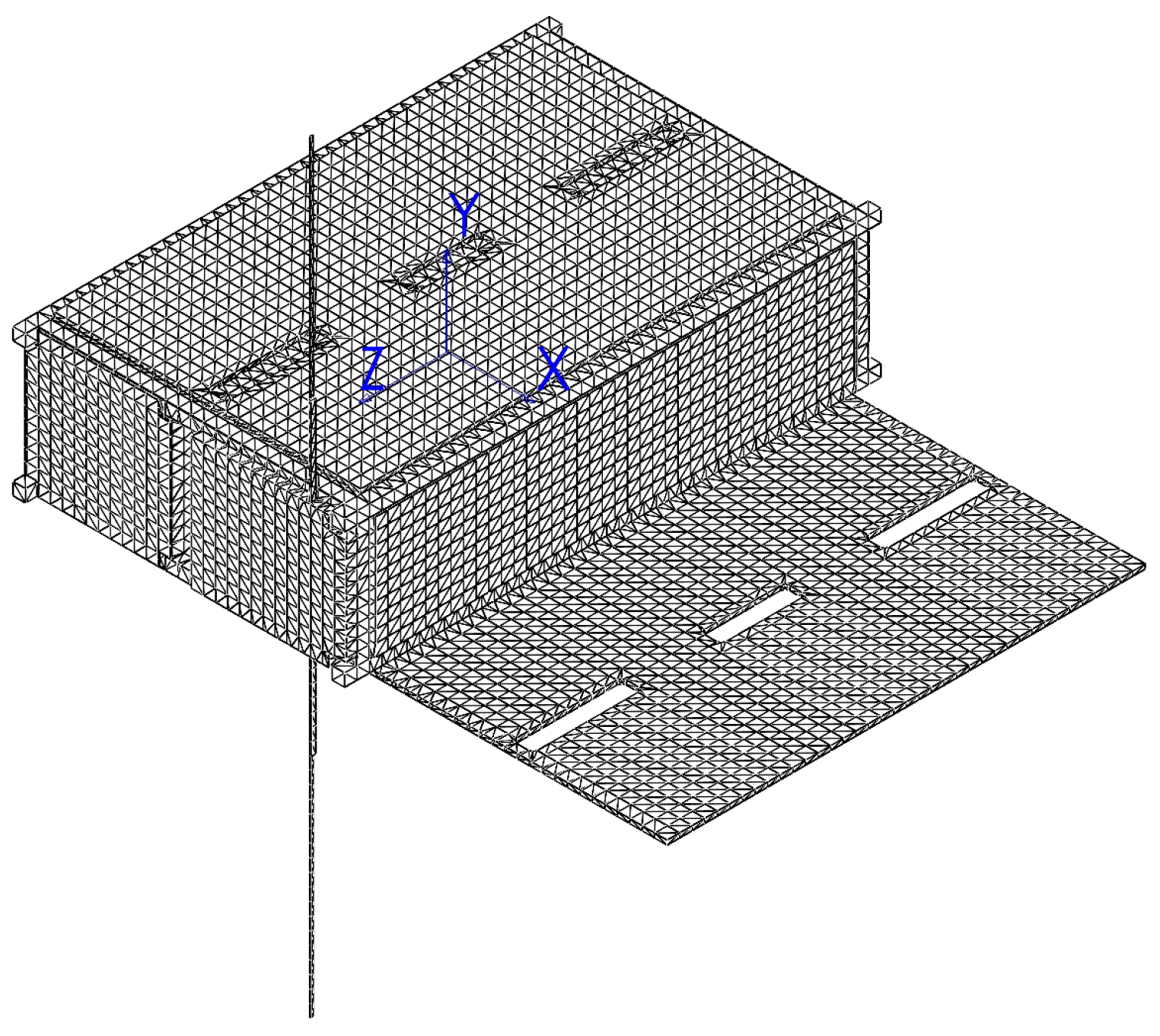
For MOVE-III without a deployed sail, the surface areas of the main structure and the deployed antenna have magnitudes of 100 and 1 mm, respectively. The simulation domain is 1 m × 1 m × 1 m, and the mesh size is 4.5 × 10⁻³ m (see Figure 7). For MOVE-III with a deployed drag sail, the simulation domain is 6 m × 6 m × 6 m for 4 m² sail cases and 8 m × 8 m × 8 m for 6.25 m² sail cases. The mesh size is 4 × 10⁻² m. In both scenarios, the surface temperature of the CubeSat is 350 K [35].

To confirm the flow regime, Knudsen numbers of the flow for MOVE-III with and without the drag sail are examined. The characteristic length of MOVE-III before deploying the sail is 0.2 m, which increases to 2.087 m after deploying the 4 m² sail and 2.609 m after deploying the 6.25 m² sail. The Knudsen numbers are then computed and presented in

Table 4. Knudsen numbers of the simulation cases.

Altitude [km]	No Sail	4 m2 Sail	6.25 m2 Sail
125	26.75	2.563	-
185	865	82.89	66.31
300	1.30 × 104	1243	994.6
450	1.73 × 105	1.66 × 104	-

.

4.2. Simulation Results and Aerodynamic Coefficients

DSMC simulations were performed based on the geometry and atmospheric data discussed in Section 2 and Section 4.1. The velocity fields of three selected attitudes at 125 km are shown in Figure 8 and Figure 9.

At orbital altitudes of 185 km and 300 km, cases of MOVE-III without deploying the sail and after deploying two sail sizes of 4 m² and 6.25 m² were simulated, respectively. The attitude of the CubeSat was set to be $\alpha =0$ and $\beta =0$. The effect of utilizing different sail sizes on the drag force and $C_D$ is shown in

Table 5. Effect of different sail sizes on drag force and drag coefficient at 185 and 300 km.

Parameter		Value
Sail size [m2]		0 (No sail)	4	6.25
Characteristic length [m]		0.2	2.087	2.609
Drag force [mN]	185 km	1.8	102.5	159.2
	300 km	0.06	5.1	7.9
Drag coefficient	185 km	2.372	2.006	1.993
	300 km	2.603	2.031	2.020

.

By comparing the data in Table 5, it is observed that the shape of the CubeSat with the deployed drag sail is the dominant factor, while the influence of sail size is relatively minor. However, it is evident that a 56% increase in sail size results in a 55% increase in drag force, leading to a greater deceleration of the CubeSat with the larger sail. Upon the installation of the 4 m² sail, the aerodynamic drag force acting on MOVE-III increases by a factor of 57 at an orbital altitude of 185 km and by a factor of 85 at 300 km compared to the case without the sail, leading to a significant reduction in deorbiting time. A further quantitative analysis of the effect of the drag sail on the deorbiting time is presented in Section 5.

A further analysis is presented to juxtapose the drag force generated by the drag sail with the thrust force of widely utilized electric thrusters, as introduced in Section 1. Given that electric thrusters represent an alternative approach to the drag sail technique, this study undertook a comparative evaluation of the drag forces derived for the two higher-altitude scenarios examined herein against the thrust forces produced by standard ion thrusters [11]. The 4 m² drag sail is capable of generating drag forces of 5.1 mN at an orbital altitude of 300 km and 0.4 mN at 450 km. Considering that vacuum arc, pulsed plasma, and microwave thrusters typically yield thrust forces of 0.01, 0.04, and 3 mN with system sizes of approximately 0.1, 1, and 5 U and weights of 0.3, 2, and 26 kg, respectively [36], the deorbiting capability of the 4 m² sail is evidently more effective than that of electric thrusters with similar dimensions and weights.

4.3. Comparison to FMF Theory

The FMF analysis of MOVE-III with and without the 4 m² drag sail for all nine attitudes listed in Table 3 is based on the parameters set in Section 4.1. Upon collecting simulation result data, the errors of FMF based on the DSMC method were readily computed (see

Table 6. Drag coefficient $C_D$ comparison and error calculation for cases of MOVE-III with deployed 4 m² sail at different orbital altitudes H.

Attitude Case			H = 125 km			H = 185 km			H = 300 km
No.	$\mathit{\alpha }$ [°]	$\mathit{\beta }$ [°]	FMF	DSMC	$\mathit{\eta }$ [%]	FMF	DSMC	$\mathit{\eta }$ [%]	FMF	DSMC	$\mathit{\eta }$ [%]
00	0	0	1.989	1.889	5.3	2.005	2.006	0.1	2.025	2.031	0.3
03	0	30	1.488	1.460	1.9	1.502	1.523	1.4	1.519	1.543	1.5
06	0	60	0.525	0.569	7.7	0.534	0.543	1.6	0.546	0.555	1.7
30	30	0	1.473	1.339	10.0	1.486	1.398	6.3	1.503	1.417	6.1
33	30	30	1.108	1.195	7.3	1.119	1.230	9.0	1.134	1.247	9.1
36	30	60	0.393	0.530	25.9	0.401	0.504	20.4	0.410	0.515	20.4
60	60	0	0.513	0.520	1.3	0.521	0.498	4.7	0.532	0.509	4.5
63	60	30	0.388	0.485	20.1	0.395	0.462	14.5	0.405	0.473	14.4
66	60	60	0.147	0.357	58.8	0.153	0.327	53.3	0.159	0.337	52.9

). According to Figure 10, FMF shows good consistency for vertical incidence cases with DSMC results for altitudes larger than or equal to 185 km. However, for large-incident-angle cases, considerable deviations from zero-angle cases are observed. Note that Cases 00 and 63 at an altitude of 240 km were simulated as a complement. Atmospheric data were also obtained from the US Standard Atmosphere (1976) [34]. Analyzing Table 6, the FMF and DSMC results at 185 km and 300 km coincide well for Cases 00, 03, 06, and 60. The errors for these cases are all no more than 5%. Cases 30 and 33 possess errors of less than 10%. Large deviations ($\eta >10\%$) are found for Cases 36, 63, and 66. By cross-checking the “angle-swap” pairs, Case 03 with 30, Case 06 with 60, and Case 36 with 63, the $C_D$ of each case group is found to be different due to the asymmetric geometry of MOVE-III. Hence, the accuracy of FMF also relies on the configuration of the test part’s surface.

GSI models of FMF only account for one-time particle–surface collisions and neglect multi-time particle–surface collisions and inter-molecular collisions. By inspecting the flow field streamlines near the surface (see Figure 8 and Figure 9), it is discovered that the translating directions of particles are changed near the surface and vary at different locations according to the geometry. As the incident angle increases, the bottom and lateral surfaces, which are shaded in zero-incident-angle cases, become exposed to the incoming flow. The normal vectors of the surface elements now have three non-zero components in the aerodynamic reference frame, thereby increasing the geometry concavity influence. Inter-molecular collisions should exist, and the basic assumption of GSI models no longer applies. Consequently, this leads to discrepancies in the FMF predictions.

Furthermore, FMF is a valuable tool for estimating the $C_D$ of LEO spacecraft under small free-stream incident angles. This method relies on analytically solving equations that are obtained through appropriate simplification assumptions. A computer only requires the input of relevant parameters (e.g., atmospheric and solar conditions) to calculate the values, which makes this a relatively fast and resource-efficient process. In contrast, no general solution to the Boltzmann Equation has been developed thus far. The DSMC method involves a reduction of real-world physical phenomena and a step-by-step reproduction of them. This process consumes a significant amount of computational resources and time. Researchers have acknowledged the efficiency advantage of the FMF method and the accuracy advantage of the DSMC method and are currently investigating ways to overcome the limitations of the DSMC method and to combine the advantages of both approaches [37].

5. Deorbiting Time Forecast

To forecast the orbit decay of the CubeSat, appropriate atmospheric and physical models are necessary. This study utilizes both a contemporary empirical periodic decay model and a fundamental orbital equation model. $C_D$ data gathered from various altitudes, as detailed in Section 4, are incorporated into the prediction process. The results suggest that the deployment of the drag sail significantly shortens the CubeSat’s deorbiting duration, which potentially contributes to the prevention and mitigation of space debris.

5.1. Atmospheric Model

The orbital decay of LEO satellites is primarily caused by their interaction with the rarefied atmosphere. Such interaction is characterized by the drag force D:

$$D=\frac{1}{2}\rho V^{2}A{C}_D$$

(2)

where $\rho$ is the atmospheric density, V is the velocity of the satellite, A is the cross-sectional area perpendicular to the direction of motion, and $C_D$ is the drag coefficient, as discussed in Section 4.

As a result, the prediction of their orbital lifetimes is dependent on the density distribution of the upper atmosphere. The density below 500 km follows an exponential distribution, with an equivalent height denoted by H (in kilometers):

$$\rho =6\times {10}^{-10}{e}^{-\frac{h-175}{H}}$$

(3)

where H is defined as $H=T/m$, and h (in kilometers) is the orbital altitude. T and m are exospheric temperature and effective atmospheric molecular mass, respectively. T reflects the universal environmental factors, including solar and geomagnetic activities [38].

$$T=900+2.5(F10.7-70)+1.5Ap$$

(4)

where $F10.7$ is the solar radio flux, and $Ap$ is the geomagnetic index. For the considered altitude regime $h\le 500$ km, the effective atmospheric molecular mass m is given by:

$$m=27-0.012(h-200)$$

(5)

which includes the actual variation in molecular mass with altitude. It also takes into account a compensation term for temperature changes over the altitude range of interest [39].

It is worth noting that the intermediate variables involved in the derivation of an atmospheric model do not align with the authentic atmospheric values. Consequently, the atmospheric density stands as the sole legitimate output value of the model.

5.2. Orbital Decay Model

The orbital period P of a circular LEO has the following relationship with the orbital radius R, which is also known as Kepler’s Third Law of Planetary Motion:

$$P^{2}GM=4{\pi }^2{R}^3$$

(6)

where G is the gravitational constant, and M is the mass of the Earth.

The reduction in the orbital period due to orbital decay caused by the rarefied atmospheric drag force is governed by

$$\frac{dP}{dt}=-3\pi R\rho \left(\frac{A_e}{m_{sat}}\right)$$

(7)

where $A_e=A{C}_D$ is the effective cross-sectional area, and $m_{sat}$ is the mass of the satellite [39].

By applying Equations (6) and (7), in conjunction with the aforementioned upper atmospheric density model (see Section 5.1), the satellite’s orbital altitude and in-orbit time can be iteratively solved to depict the orbital decay. These equations form the basis of what is commonly referred to as the periodic decay model.

Given that typical applications of the periodic decay model often assume a constant $C_D$, and considering that $C_D$ in this study fluctuates with the orbital altitude, it becomes imperative to corroborate the applicability of the periodic decay model to scenarios with a variable $C_D$. To achieve this, we employ a fundamental approach, namely, the orbital equation model [40]. This model contains both kinematic and kinetic equations of particle motion, spanning from Equations (8) to (13). In this work, the Earth’s rotation is neglected.

$$\dot{\delta }=\frac{Vcos\gamma cos\chi }{Rcos\lambda }$$

(8)

$$\dot{\lambda }=\frac{Vcos\gamma sin\chi }{R}$$

(9)

$$\dot{R}=Vsin\gamma$$

(10)

$$\dot{V}=-\frac{GM}{R^2}sin\gamma -\frac{D}{m}$$

(11)

$$\dot{\gamma }=(\frac{V}{R}-\frac{GM}{R^{2}V})cos\gamma$$

(12)

$$\dot{\chi }=-\frac{Vcos\gamma cos\chi tan\lambda }{R}$$

(13)

where $\delta$ and $\lambda$ are the longitude and latitude, respectively, R is the orbital radius, $\gamma$ is the flight-path angle, and $\chi$ is the heading angle [40].

In practice, satellites with mass-to-area ratios less than 100 kg/m² experience a relatively short lifespan of a few hours when orbiting at altitudes below 180 km. Therefore, a satellite is considered to have completed its deorbiting process once it reaches an altitude of 175 km.

As depicted in Figure 11, the prediction results indicate that the decay process is influenced by the $C_D$ value. When compared to scenarios with a constant $C_D$, the deorbiting time in cases where $C_D$ varies is slightly shorter. This is attributed to the reduction in $C_D$ as the CubeSat descends to lower altitudes. Furthermore, both the periodic decay model and the orbital equation model are employed to forecast the trajectory of MOVE-III equipped with a 4 m² drag sail, serving as a means of validation. The variable $C_D$ values, corresponding to different orbital altitudes, are derived through interpolation from the results presented in Section 4.

5.3. The Assessment of the Drag Sail

The DSMC results show that the $C_D$ of LEO spacecraft varies with the change in orbital altitude. Due to the aerodynamic stability of the drag sail [41], the only attitude that needs to be considered is Case 00, i.e., $\alpha =0$, $\beta =0$. The $C_D$ values of this attitude at different altitudes are obtained in Table 6 of Section 4.3. These data are interpolated over the altitude range. The initial altitude is set to 500 km, which is a typical LEO altitude and the likely operating orbit of MOVE-III. To be concise, the perturbation due to the orbital environment is ignored, and parameters are assumed to be constant. The mass of MOVE-III is 7 kg, the cross-sectional area is 0.039 m² (without drag sail) or 4.36 m² (with drag sail), the solar radio flux is 160 SFU, and the geomagnetic index is 5. The altitude decrease with time is then calculated and shown in Figure 12.

At an initial orbital altitude of 500 km, upon deploying the 4 m² drag sail, the deorbiting time of MOVE-III plummeted from 1091 days (equivalent to approximately three years) with no sail deployed to a mere 12 days. This significant reduction in deorbiting time confirms that the drag sail effectively reduces the time taken for CubeSats to deorbit.

It is worth noting that the solar radiation pressure (SRP) effect also potentially perturbs the deorbit trajectory of the CubeSat, especially at high altitudes around 450 km [42]. However, it is a complex coupled problem to include both aerodynamic force and SRP effects in an analytical model. Since the literature indicates that the drag force is the dominant factor in LEO compared with the SRP effect [43], the influence of SRP will be discussed in future works and was not considered in this study.

6. Conclusions

This study examines the detailed drag characteristics of spacecraft using the DSMC method, particularly exploring the potential utility of a deorbit drag sail for the scientific research CubeSat MOVE-III. We developed a simplified simulation model for MOVE-III without the sail and conducted both FMF and 3D DSMC simulations across varying attitudes at altitudes of 125 km, 185 km, and 300 km. (A sentence is deleted here.) Our results validate the FMF method as a credible alternative to the DSMC method in the free molecular flow regime at altitudes of 185 km and 300 km, particularly when the free stream incident angle is neutral ($\alpha =0$ and $\beta =0$). Nonetheless, the precision of FMF under non-neutral incident angles is contingent upon the specific surface geometry characteristics within the free stream. At a constant alatitude, FMF’s accuracy improves with reduced concavity in the geometry. At 125 km, the flow regime becomes transitional, rendering FMF less dependable. Consequently, under specified conditions, FMF emerges as a viable, less resource-intensive substitute for the DSMC method.

Our research also uncovers that the dimensions of the drag sail marginally influence the drag coefficient ($C_D$) at a fixed altitude. Deploying the sail does reduce $C_D$, but it significantly enlarges the CubeSat’s cross-sectional area, amplifying the deorbiting force to levels akin to an electric thruster. This surge in drag force dramatically shortens the re-entry duration by two orders of magnitude, from around ${10}^3$ days to merely 10 days. This study further emphasizes that the accurate computation of $C_D$ is vital for reliably predicting the deorbiting timeframe.

Future endeavors should aim to delineate the specific conditions under which FMF proves to be a reliable and practical tool. This study suggests that such conditions could encompass factors including the characteristics of the orbital atmosphere, which are influenced by the satellite’s altitude, as well as the spacecraft’s external configuration, which is shaped by its orientation and surface features, such as concavity. Additionally, the coupled effect of aerodynamics and SRP on deorbiting trajectories is critical for precise predictions at higher altitudes, which will be further explored in subsequent research.

References

- Poghosyan, A.; Golkar, A. CubeSat evolution: Analyzing CubeSat capabilities for conducting science missions. Prog. Aerosp. Sci. 2017, 88, 59–83. [Google Scholar] [CrossRef]
- Woellert, K.; Ehrenfreund, P.; Ricco, A.J.; Hertzfeld, H. Cubesats: Cost-effective science and technology platforms for emerging and developing nations. Adv. Space Res. 2011, 47, 663–684. [Google Scholar] [CrossRef]
- McCreary, L. A satellite mission concept for high drag environments. Aerosp. Sci. Technol. 2019, 92, 972–989. [Google Scholar] [CrossRef]
- Liou, J.C.; Johnson, N. Risks in space from orbiting debris. Science 2006, 311, 340–341. [Google Scholar] [CrossRef]
- Vallado, D.A.; Finkleman, D. A critical assessment of satellite drag and atmospheric density modeling. Acta Astronaut. 2014, 95, 141–165. [Google Scholar] [CrossRef]
- Serfontein, Z.; Kingston, J.; Hobbs, S.; Holbrough, I.E.; Beck, J.C. Drag augmentation systems for space debris mitigation. Acta Astronaut. 2021, 188, 278–288. [Google Scholar] [CrossRef]
- Gaglio, E.; Bevilacqua, R. Time Optimal Drag-Based Targeted De-Orbiting for Low Earth Orbit. Acta Astronaut. 2023, 207, 316–330. [Google Scholar] [CrossRef]
- Stohlman, O.R.; Lappas, V. Deorbitsail: A deployable sail for de-orbiting. In Proceedings of the 54th AIAA/ASME/ASCE/AHS/ASC Structures, Structural Dynamics, and Materials Conference, Boston, MA, USA, 8–11 April 2013. [Google Scholar] [CrossRef]
- Visagie, L.; Lappas, V.; Erb, S. Drag sails for space debris mitigation. Acta Astronaut. 2015, 109, 65–75. [Google Scholar] [CrossRef]
- Netzer, E.; Kane, T.R. Electrodynamic forces in tethered satellite systems part I: System control. IEEE Trans. Aerosp. Electron. Syst. 1994, 30, 1031–1038. [Google Scholar] [CrossRef]
- Holste, K.; Dietz, P.; Scharmann, S.; Keil, K.; Henning, T.; Zschätzsch, D.; Reitemeyer, M.; Nauschütt, B.; Kiefer, F.; Kunze, F.; et al. Ion thrusters for electric propulsion: Scientific issues developing a niche technology into a game changer. Rev. Sci. Instrum. 2020, 91, 061101. [Google Scholar] [CrossRef]
- Lappas, V.; Adeli, N.; Visagie, L.; Fernandez, J.; Theodorou, T.; Steyn, W.; Perren, M. CubeSail: A low cost CubeSat based solar sail demonstration mission. Adv. Space Res. 2011, 48, 1890–1901. [Google Scholar] [CrossRef]
- Long, A.C.; Spencer, D.A. Stability of a deployable drag device for small satellite deorbit. In Proceedings of the AIAA/AAS Astrodynamics Specialist Conference, Long Beach, CA, USA, 13–16 September 2016. [Google Scholar]
- Fernandez, J.M.; Visagie, L.; Schenk, M.; Stohlman, O.R.; Aglietti, G.S.; Lappas, V.J.; Erb, S. Design and development of a gossamer sail system for deorbiting in low earth orbit. Acta Astronaut. 2014, 103, 204–225. [Google Scholar] [CrossRef]
- Serfontein, Z.; Kingston, J.; Hobbs, S.; Impey, S.A.; Aria, A.I.; Holbrough, I.E.; Beck, J.C. Effects of long-term exposure to the low-earth orbit environment on drag augmentation systems. Acta Astronaut. 2022, 195, 540–546. [Google Scholar] [CrossRef]
- Qu, Q.; Xu, M.; Luo, T. Design concept for In-Drag Sail with individually controllable elements. Aerosp. Sci. Technol. 2019, 89, 382–391. [Google Scholar] [CrossRef]
- Li, Y.; Fan, X. Development of PW-Sat2 CubeSat’s deorbiting sail and the on-orbit verification. Spacecr. Environ. Eng. 2020, 37, 414–420. [Google Scholar] [CrossRef]
- Harkness, P.; McRobb, M.; Lützkendorf, P.; Milligan, R.; Feeney, A.; Clark, C. Development status of AEOLDOS-A deorbit module for small satellites. Adv. Space Res. 2014, 54, 82–91. [Google Scholar] [CrossRef]
- Shmuel, B.; Hiemstra, J.; Tarantini, V.; Singarayar, F.; Bonin, G.; Zee, R. The Canadian Advanced Nanospace eXperiment 7 (CanX-7) Demonstration Mission: De-Orbiting Nano- and Microspacecraft. In Proceedings of the 26th Annual AIAA/USU Conference on Small Satellites, Logan, UT, USA, 13–16 August 2012. [Google Scholar]
- Nikolajsen, J.A.; Kristensen, A.S. Self-deployable drag sail folded nine times. Adv. Space Res. 2021, 68, 4242–4251. [Google Scholar] [CrossRef]
- Mostaza Prieto, D.; Graziano, B.P.; Roberts, P.C. Spacecraft drag modelling. Prog. Aerosp. Sci. 2014, 64, 56–65. [Google Scholar] [CrossRef]
- Moe, K.; Moe, M.M. Gas-surface interactions and satellite drag coefficients. Planet. Space Sci. 2005, 53, 793–801. [Google Scholar] [CrossRef]
- Bird, G. Molecular Gas Dynamics and the Direct Simulation of Gas Flows, 2nd ed.; Oxford Science Publications: Oxford, UK, 1994. [Google Scholar]
- Oikonomidou, X.; Karagiannis, E.; Still, D.; Strasser, F.; Firmbach, F.S.; Hettwer, J.; Schweinfurth, A.G.; Pucknus, P.; Menekay, D.; You, T.; et al. MOVE-III: A CubeSat for the detection of sub-millimetre space debris and meteoroids in Low Earth Orbit. Front. Space Technol. 2022, 3, 933988. [Google Scholar] [CrossRef]
- Horstmann, A.; Wiedemann, C.; Braun, V.; Matney, M.; Vavrin, A.; Gates, D.; Seago, J.; Anz-Meador, P.; Wiedemann, C.; Lemmens, S. Flux comparison of MASTER-8 and ORDEM 3.1 modelled space debris population. In Proceedings of the 8th European Conference on Space Debris, Virtual, 20–23 April 2021. [Google Scholar]
- Igenbergs, E.; Hüdepohl, A.; Uesugi, K.; Hayashi, T.; Svedhem, H.; Iglseder, H.; Koller, G.; Glasmachers, A.; Grün, E.; Schwehm, G.; et al. The Munich dust counter—A cosmic dust experiment on board of the Muses-A mission of Japan. In Origin and Evolution of Interplanetary Dust: Proceedings of the 126th Colloquium of the International Astronomical Union, Held in Kyoto, Japan, 27–30 August 1990; Springer: Dordrecht, The Netherlands, 1991; pp. 45–48. [Google Scholar]
- Marín, A.; Sebastiaõ, I.B.; Tamrazian, S.; Spencer, D.; Alexeenko, A. DSMC-SPARTA aerodynamic characterization of a deorbiting CubeSat. In Proceedings of the 31ST International Symposium on Rarefied Gas Dynamics: Rgd31, Glasgow, UK, 23–27 July 2018; AIP Publishing: Melville, NY, USA, 2019; Volume 2132. [Google Scholar] [CrossRef]
- Sentman, L.H. Free Molecule Flow Theory and Its Application to the Determination of Aerodynamic Forces; Technical Report AD0265409; Lockheed Missiles and Space Co., Inc.: Sunnyvale, CA, USA, 1961. [Google Scholar]
- Mungiguerra, S.; Zuppardi, G.; Savino, R. Rarefied aerodynamics of a deployable re-entry capsule. Aerosp. Sci. Technol. 2017, 69, 395–403. [Google Scholar] [CrossRef]
- Liang, J.; Li, Z.; Li, X.; Shi, W. Monte carlo simulation of spacecraft reentry aerothermodynamics and analysis for ablating disintegration. Commun. Comput. Phys. 2018, 23, 1037–1051. [Google Scholar] [CrossRef]
- Jiang, Y.; Zhang, J.; Tian, P.; Liang, T.; Li, Z.; Wen, D. Aerodynamic drag analysis and reduction strategy for satellites in Very Low Earth Orbit. Aerosp. Sci. Technol. 2023, 132, 108077. [Google Scholar] [CrossRef]
- Chen, S.; Stemmer, C. Modeling of Thermochemical Nonequilibrium Flows Using Open-Source Direct Simulation Monte Carlo Kernel SPARTA. J. Spacecr. Rocket. 2022, 59, 1634–1646. [Google Scholar] [CrossRef]
- Mehta, P.M.; Paul, S.N.; Crisp, N.H.; Sheridan, P.L.; Siemes, C.; March, G.; Bruinsma, S. Satellite drag coefficient modeling for thermosphere science and mission operations. Adv. Space Res. 2023, 72, 5443–5459. [Google Scholar] [CrossRef]
- NOAA. U.S. Standard Atmosphere 1976; National Oceanic and Atmospheric Administration: Washington DC, USA, 1976. [Google Scholar]
- Markelov, G.; Kashkovsky, A.; Ivanov, M. Space station Mir aerodynamics along the descent trajectory. J. Spacecr. Rocket. 2001, 38, 43–50. [Google Scholar] [CrossRef]
- Tian, L.; Wang, S.; Gao, J.; Meng, W.; Tian, K.; Wu, C. Development and Application of Micro-electric Propulsion System. Vacuum 2021, 58, 66–75. [Google Scholar] [CrossRef]
- Falchi, A.; Minisci, E.; Vasile, M.; Rastelli, D.; Bellini, N. DSMC-based Correction Factor for Low-fidelity Hypersonic Aerodynamics of Re-entering Objects and Space Debris. In Proceedings of the 7th European Conference for Aeronautics and Space Sciences, Milan, Italy, 3–6 July 2017. [Google Scholar]
- Guo, J.; Gu, S.; Chen, D. Analysis of the Effect of Space Environment on Shenzhou Spaceship Orbit Attenuation. Spacecr. Eng. 2008, 17, 59–63. [Google Scholar]
- Jursa, A.S. Handbook of Geophysics and Space Environment; Hanscom Air Force Base: Hanscom AFB, MA, USA, 1985. [Google Scholar]
- Kumar, M.; Tewari, A. Trajectory and attitude simulation for aerocapture and aerobraking. J. Spacecr. Rocket. 2005, 42, 684–693. [Google Scholar] [CrossRef]
- Black, A.; Spencer, D.A. DragSail systems for satellite deorbit and targeted reentry. J. Space Saf. Eng. 2020, 7, 397–403. [Google Scholar] [CrossRef]
- Tan, B.; Yuan, Y.; Zhang, B.; Hsu, H.Z.; Ou, J. A new analytical solar radiation pressure model for current BeiDou satellites: IGGBSPM. Sci. Rep. 2016, 6, 32967. [Google Scholar] [CrossRef]
- Johnson, L.; Alhorn, D.; Boudreaux, M.; Casas, J.; Stetson, D.; Young, R. Solar and Drag Sail Propulsion: From Theory to Mission Implementation; Technical Report; National Aeronautics and Space Administration: Washington DC, USA, 2014. [Google Scholar]
Figure 1.
Isometric view of the front (a) and back (b) of the simplified assembly model of MOVE-III.
Figure 2.
Configuration of 4 m2 (a,b) and 6.25 m2 (c,d) sails.
Figure 3.
Schematic of gas–surface interaction.
Figure 4.
of the flat plate with the change in altitude.
Figure 5.
Isometric view of the front (a) and back (b) of MOVE-III’s panel construction.
Figure 6.
Panel constructions of 4 m2 (a,b) and 6.25 m2 (c,d) sail cases.
Figure 7.
Surface mesh panels of deployed MOVE-III.
Figure 8.
Velocity field of MOVE-III at altitude of 125 km and attitude of , .
Figure 9.
Velocity fields of three selected attitudes at 125 km.
Figure 10.
Agreement comparison of FMF and DSMC results of MOVE-III with deployed 4 m2 sail at certain attitudes.
Figure 11.
Deorbiting trajectory comparison for different and decay prediction models.
Figure 12.
Deorbiting trajectories for both no−sail and deployed−sail cases.