Period-Multiplying Bifurcations in the Gravitational Field of Asteroids

Abstract

Periodic orbit families around asteroids serve as potential trajectories for space probes, mining facilities, and deep space stations. Bifurcations of these families provide additional candidate orbits for efficient trajectory design around asteroids. While various bifurcations of periodic orbit families around asteroids have been extensively studied, period-multiplying bifurcations have received less attention. This paper focuses on studying period-multiplying bifurcations of periodic orbit families around asteroids. In particular, orbits with periods of approximately 7 and 17 times that of the rotational period of asteroid 216 Kleopatra were computed. The computation of high-period orbits provides insights into the numerical aspects of simulating long-duration trajectories around asteroids. The previous literature uses single-shooting and multiple-shooting methods to compute bifurcations of periodic orbit families around asteroids. Computational difficulties were encountered while using the shooting methods to obtain period-multiplying bifurcations of periodic orbit families around asteroids. This work used the Legendre–Gauss collocation method to compute period-multiplying bifurcations around asteroids. This study recommends the use of collocation methods to obtain long-duration orbits around asteroids when computational difficulties are encountered while using shooting methods.

1. Introduction

There is a growing interest in the study of orbital mechanics around asteroids, as asteroids are rich sources of carbonaceous, silicate, and metallic resources. The profitable mining of these resources requires a thorough understanding of the orbital mechanics around asteroids. A crucial prerequisite for this understanding is an accurate gravitational field model, as the fidelity of the simulated orbital dynamics is directly tied to the quality of the gravitational model employed.

Numerous space missions have been conducted to visit various asteroids (for example, NASA’s Shoemaker to asteroid 433 Eros [1], JAXA’s Hayabusa probe to asteroid (25143) Itokawa [2], the Chinese National Space Administration’s (CNSA) Chang’e-2 to asteroid (4179) Toutatis [3], the Rosetta mission to comet 67P [4], NASA’s OSIRIX-Rex to asteroid Bennu [5], and JAXA’s Hayabusa 2 probe to asteroid 162173 Ryugu [6]). These missions involved a close fly-by, landing on the asteroid’s surface, and asteroid surface material sample return (see [7,8,9] for a detailed study on asteroid fly-by, landing, and sample return missions), yielding extensive imaging of the asteroids. The collected image data were then used to determine the asteroid’s polyhedral shape and density.

The polyhedral shape of an asteroid is the polyhedral approximation of the asteroid obtained through the discretization of the asteroid’s surface into polygons. Fujiwara et al. obtained asteroid 25143 Itokawa’s polyhedral shape using data from JAXA’s Hayabusa mission [10] to 25143 Itokawa. Though space missions provide valuable data, it is not feasible to conduct space missions to every asteroid for which the study of orbital mechanics is sought. Radar observations and lightcurve data are used to obtain the polyhedral shapes of asteroids to which no space missions have been conducted. Ostro et al. constructed a high-resolution polyhedral shape of asteroid 216 Kleopatra consisting of 4096 edges and 2048 triangular faces using data from radar observations [11]. Polyhedral models can also be obtained from lightcurve inversion techniques [12]. The polyhedral shape is used to construct the gravitational field of the asteroid.

Werner and Scheeres derived closed-form expressions for the gravitational fields of bodies bounded by a polygonal surface and, in particular, computed the gravitational field of asteroid 433 Eros by using its polyhedral shape [13]. The closed-form expressions in [13] are known as the polyhedral model of gravitation for asteroids. The polyhedral model of gravitation provides the required gravitational field information to study orbital motion around asteroids.

The study of orbital mechanics around an asteroid involves the computation of trajectories that a spacecraft would follow when the spacecraft is under the gravitational influence of the asteroid. Since no closed-form solutions are available, trajectories are computed by employing numerical integration schemes (see [14] for details on numerical integration schemes used in astrodynamical problems).

The computation of periodic orbit families and their bifurcations is a current area of focus in the study of orbital mechanics around asteroids, as these orbits serve as potential trajectories to station spacecraft exploring an asteroid. A periodic orbit family is a continuous set of periodic orbits parameterized by a single parameter [15]. Lara and Peláez developed an analytic continuation technique to obtain periodic orbit families for astrodynamical systems with three degrees of freedom [16]. The computation of periodic orbits not only provides suitable trajectories for asteroid missions but also offers insights into selecting appropriate numerical methods for studying orbital motion. For example, Pal et al. showed showed that explicit Euler integration gave inaccurate results for periodic trajectories involved in the relative motion of two spacecraft in the Earth’s gravitational field and recommended the use of the Lindstedt–Poincare method for the accurate computation of periodic trajectories [17]. Zeng and Liu used an indirect method based on the optimal control framework to obtain periodic orbits around elongated asteroids [18]. Yu et al. introduced the hierarchical grid search method to compute periodic orbits around asteroids [19]. Using the hierarchical grid search method, Yu et al. computed 29 periodic orbit families around the asteroid 216 Kleopatra [19]. Periodic orbits around various other asteroids were also computed using the hierarchical grid search method [20,21,22,23,24].

The bifurcations of periodic orbit families around asteroids provide the structure of periodic orbit families around the asteroid. The structure of periodic orbit families refers to the relationship between the various computed periodic orbit families. These relationships could be of two types. In the first type, two periodic orbit families are connected through a common periodic orbit that is an extremum with respect to the period, making the families part of a larger single periodic orbit family. In the second type of relationship, two periodic orbit families are not part of a larger family but share a common periodic orbit.

The bifurcation of periodic orbit families helps locate points of extrema along the periodic orbit family with respect to the period or energy; such kinds of bifurcations are called first-kind bifurcations. The first kind of bifurcation of periodic orbit families around asteroids has been well studied in the literature [25,26,27]. Ni et al. showed that multiple first-kind bifurcations occur along a periodic orbit family around an asteroid [28]. The bifurcation of periodic orbit families also helps to identify additional periodic orbit families; such kinds of bifurcations are called second-kind bifurcations. Jiang and Baoyin studied tangent bifurcations in the gravitational field of asteroids 216 Kleopatra and 433 Eros [29]. Tangent bifurcations are a particular type of second-kind bifurcation.

Period-multiplying bifurcations are another type of second-kind bifurcation. Period-multiplying bifurcations of periodic orbit families are bifurcations in which the periodic orbit family intersecting the bifurcating orbit has approximately integer multiples of periods of the other periodic orbit family that contains the bifurcating orbit. Vanderbauwhede proved that period-multiplying bifurcations of any integer multiple exist for a periodic orbit family in Hamiltonian systems [30]. Li et al. computed period-multiplying bifurcations of periodic orbit families in the Jupiter–Ganymede system using the shooting method [31]. The computed period-multiplying orbits were leveraged for low-energy transfers within the Jupiter–Ganymede system. Period-multiplying bifurcations of periodic orbit families provide more candidates for trajectory design.

The numerical computation of period-multiplying bifurcations of periodic orbit families is difficult because of the large time-scale separation in the underlying dynamics. Pellegrini and Russell studied the computation of long-period periodic orbits in the Earth–Moon gravitational system and recommended appropriate numerical integration schemes to compute the trajectories accurately [32]. On the other hand, the literature has paid little attention to period-multiplying bifurcations around asteroids. Liu et al. were able to locate period-doubling bifurcations around asteroids Bennu and Steins [26]. Brown and Scheeres located and computed period-multiplying bifurcations up to integer five around the asteroid Bennu [33]. However, computational issues were reported while using the shooting methods to obtain period-multiplying bifurcations in certain locations, and period-multiplying bifurcations of integers greater than five were neither located nor computed. The location and computation of period-multiplying bifurcations of larger integers can provide more periodic orbits that can be leveraged for trajectory design. Their geometry and stability properties can make them more attractive than the parent periodic orbit family that they bifurcated from.

This paper aims to locate and compute period-multiplying bifurcations of periodic orbit families around asteroids. The vertical orbit family emanating from one of the equilibrium points of 216 Kleopatra [34] is taken as the parent periodic orbit family for which period-multiplying bifurcations are sought. The parent periodic orbit family is computed through the shooting method. Period-multiplying bifurcations along the parent periodic orbit family are located. The shooting method is predominantly used in the existing literature for computing periodic orbit families around asteroids [35]. However, it is found in this work that the shooting methods fail to compute period-multiplying bifurcations of periodic orbit families around asteroids accurately. This work uses the Legendre–Gauss collocation method to compute the period-multiplying bifurcations of periodic orbit families around asteroids.

The study in this paper involves the asteroid 216 Kleopatra, but the methods applied in this paper are general and can be applied to any other asteroid. Kleopatra was chosen as it is representative of a large number of naturally elongated asteroids in the solar system, like 433 Eros, 4769 Castalia, 243 Ida, and 4179 Toutatis [19,36]. The choice of Kleopatra is justified by the cohesive strength that helps it to avoid body disruption, making Kleopatra an ideal candidate for space missions [36]. Radar observations of Kleopatra and subsequent estimates from radar observations show that the interior of Kleopatra has an unconsolidated rubber pile structure [11], supporting the findings that Kleopatra’s cohesive strength avoids body disruptions [36]. The previous literature [33] studied period-multiplying bifurcations around much smaller and nearly axisymmetrical asteroid Bennu. Period-multiplying bifurcations of periodic orbit families around larger naturally elongated asteroids have not been studied in the literature.

The following are the objectives of this paper: (1) The computation of the vertical periodic orbit family emanating from an equilibrium point of Kleopatra. (2) Locating period-multiplying bifurcations in the computed vertical periodic orbit family. (3) Using the Legendre–Gauss collocation scheme to compute the located period-multiplying bifurcations.

The following are the methodologies used in this paper: (1) The shooting method is used to obtain the vertical periodic orbit family. (2) High fidelity numerical integrators—MATLAB’s ode-78 or ode-89—are used in the shooting methods. (3) The Legendre–Gauss collocation scheme [37] is used to compute the period-multiplying bifurcations of the vertical periodic orbit family.

The following are the contributions of the paper: (1) The computation of high-period orbits through period-multiplying bifurcations of periodic orbit families around asteroids. Previous literature using the hierarchical grid search method computed periodic orbits with a maximum period of 3 times the rotational period of asteroids [19]. This work found periodic orbits of periods 6 and 13 times the rotational period of the asteroid Kleopatra by computing period 7- and period 17-multiplying bifurcations of the vertical periodic orbit family around the asteroid Kleopatra. (2) The demonstration of the success of collocation schemes in studying orbital mechanics around asteroids, making collocation schemes a reliable method to study orbital mechanics around asteroids when shooting methods fail. Previous literature uses shooting methods to compute periodic orbit families (see, e.g., [19,29]). Computational difficulties were reported when using the shooting method to obtain period-multiplying bifurcations of periodic orbit families around asteroid Bennu [33]. This work used the Legendre–Gauss collocation method as an alternative to the shooting method to compute period-multiplying bifurcations of periodic orbit families around asteroids.

Previous literature only studied tangent bifurcations of periodic orbits around asteroids (see [25,26,27,28,29]). Period-multiplying bifurcations of periodic orbit families around asteroids have only been gaining interest recently. Brown and Scheeres could only compute period-multiplying bifurcations of integer five and less [33]. Computational difficulties were a reason for the failure to compute higher period-multiplying bifurcations. This paper proposes the Legendre–Gauss collocation scheme to overcome the computational difficulties in computing higher period-multiplying bifurcations. As an application of the proposed methodology, period 7 and period 17 bifurcations of the vertical periodic orbit family were successfully computed using the Legendre–Gauss collocation scheme. This paper demonstrates the successful application of collocation techniques to solve orbital mechanics problems around asteroids. Specifically, the Legendre–Gauss collocation method is proposed as an alternative to shooting methods to obtain long-duration orbits around asteroids when computational difficulties are encountered while using shooting methods.

2. Governing Equations

The equation governing the motion of spacecraft in the gravitational field of a uniformly rotating asteroid is given in the body-fixed frame of the asteroid as

$$\ddot{\mathit{r}}+2\mathit{\omega }\times \dot{\mathit{r}}=\nabla U-\mathit{\omega }\times \left(\mathit{\omega }\times \mathit{r}\right)$$

(1)

where $\mathit{\omega }$ and U are the angular velocity and the gravitational potential of the asteroid, respectively. In Equation (1), $\mathit{r}$ represents the position vector of the spacecraft with respect to the center of mass of the asteroid, and the derivatives are with respect to the body-fixed frame. The ordinary differential equation (Equation (1)) is conservative and autonomous.

Equation (1) can be written in the following form by defining the effective potential of the rotating asteroid:

$$\ddot{\mathit{r}}+2\mathit{\omega }\times \dot{\mathit{r}}=\nabla V$$

(2)

where $V=-{\displaystyle \frac{1}{2}}\left(\mathit{\omega }\times \mathit{r}\right)·\left(\mathit{\omega }\times \mathit{r}\right)+U$ is the effective potential of the asteroid. The energy or the Jacobi constant of the governing equation (Equation (2)) is given as follows:

$$C=V\left(\mathit{r}\right)+{\displaystyle \frac{1}{2}}\dot{\mathit{r}}·\dot{\mathit{r}}$$

(3)

The gravitational potential U of an asteroid and its corresponding gradients can be obtained through the polyhedral model of gravitation. Towards this, the asteroid is approximated as a homogeneous polyhedron. The gravitational field of the resulting homogeneous polyhedron represents the asteroid’s gravitational field. The work in this paper uses the gravitational potential of a homogeneous polyhedron with triangular facets. The expressions for the gravitational potential, its gradient, and double gradient can be found in [13].

This paper uses the asteroid Kleopatra as an example to demonstrate the computations of orbital motion around asteroids. The asteroid Kleopatra represents a large group of prolate dumb-like-shaped asteroids in the solar system [19]. Kleopatra represents a large number of naturally elongated asteroids whose gravitational field cannot be accurately computed by the classical spherical harmonics model [36]. The classical spherical harmonics model diverges when applied to compute the gravitational field near the surface of naturally elongated asteroids. Previous literature [33] computed period-multiplying bifurcations of periodic orbit families around the small asteroid Bennu. This work chose a much larger asteroid Kleopatra to study period-multiplying bifurcations. The high-resolution polyhedral model of Kleopatra derived in [11] consists of 4092 edges and 2048 triangular faces. The work in this paper used this high-resolution model for Kleopatra.

3. Equilibrium Points and Their Stability

Equilibrium points are the most straightforward possible solutions to Equation (1)—the equation governing the motion of spacecraft around a rotating asteroid. Equilibrium points are stationary solutions given by the zeros of the effective gravitational field (right-hand side of Equation (1)) [19]. Zeng et al. and Wen and Zeng computed equilibrium points around asteroids using the finite element model and the dipole segment model, respectively [38,39].

3.1. Computation of Equilibrium Points

The equilibrium points of the governing equation (Equation (1)) are obtained by denoting $\dot{\mathit{r}}=\mathbf{0}$ and $\ddot{\mathit{r}}=\mathbf{0}$ and solving the following resulting equation for $\mathit{r}$.

$$\mathit{\omega }\times \left(\mathit{\omega }\times \mathit{r}\right)=-\nabla U\left(\mathit{r}\right)$$

(4)

No closed-form solutions exist to Equation (4). The non-linear equation has multiple solutions [40]. Wang et al. calculated the total number of equilibrium points for several asteroids [40]. Specifically, for Kleopatra, four equilibrium points are outside the body and three are inside it. Jiang calculated the position of these four exterior equilibrium points using Newton’s iteration method [34]. The initial locations of the equilibrium points in [34] are calculated as the critical points of the effective potential in the equatorial plane of Kleopatra, since Kleopatra is nearly symmetric about the equatorial plane [34]. This method fails for other asteroids that are equatorially asymmetrical (e.g., 25143 Itokawa). This paper used particle swarm optimization (PSO) [41] to obtain the approximate locations of the equilibrium points of Kleopatra. An iterative root-solving method was then used to correct the obtained location of multiple solutions to the required tolerance.

3.2. Stability of Equilibrium Points

The stability of an equilibrium point is the behavior of solutions to Equation (1) that lie close to the equilibrium point. It can be determined by inspecting the solutions of the linear variational equation of Equation (1) about the equilibrium point.

Let $\mathit{v}={\left[\mathit{r},\dot{\mathit{r}}\right]}^{\mathrm{T}}$, where $\mathit{r}={\left[x,y,z\right]}^{\mathrm{T}}$ and $\dot{\mathit{r}}={\left[\dot{x},\dot{y},\dot{z}\right]}^{\mathrm{T}}$. The second-order governing equation of motion in Equation (1) is written more compactly as

$$\dot{\mathit{v}}=\left[\begin{array}{ccc}\mathbf{0}& & \mathbf{I}\\ \\ -\mathbf{\Omega }\mathbf{\Omega }& & -2\mathbf{\Omega }\end{array}\right]\mathit{v}+\left[\begin{array}{c}\mathbf{0}\\ \\ \nabla U\end{array}\right]$$

(5)

where $\mathbf{0}$ and $\mathit{I}$ are the zero and identity matrices of order three, respectively, and $\mathbf{\Omega }$ is the cross-product matrix containing the body-fixed frame components of the angular velocity of the asteroid.

The linear variational equation about an equilibrium point of the non-linear Equation (5) is

$$\Delta \dot{\mathit{v}}=\left[\begin{array}{ccc}\mathbf{0}& & \mathit{I}\\ \\ -\mathbf{\Omega }\mathbf{\Omega }-\nabla \nabla U(x_{\mathrm{eq}},y_{\mathrm{eq}},z_{\mathrm{eq}})& & -2\mathbf{\Omega }\end{array}\right]\Delta \mathit{v}$$

(6)

where $\nabla \nabla U(x_{\mathrm{eq}},y_{\mathrm{eq}},z_{\mathrm{eq}})$ is the Hessian matrix of the gravitational potential evaluated at an equilibrium point. The matrix on the right-hand side of Equation (6) is called the system matrix.

The eigenspectra of the linear system of differential equation (Equation (6)) are linear invariant subspaces corresponding to the eigenvalues of the system matrix. The center subspaces are the eigenspaces corresponding to pairs of purely imaginary eigenvalues of the system matrix. This work used the center subspaces of the equilibrium points to generate small-amplitude periodic orbits around equilibrium points.

4. Periodic Orbits

Consider a system of autonomous ordinary differential equations

$$\dot{\mathit{v}}=\mathit{f}\left(\mathit{v}\right)$$

(7)

where $\mathit{X}\in {\mathbb{R}}^6$ and $f:{\mathbb{R}}^6\to {\mathbb{R}}^6$ is smooth.

The following equations form the initial value problem to the above differential equation.

$$\begin{array}{ccc}\hfill \dot{\mathit{v}}& =& \mathit{f}\left(\mathit{v}\right)\hfill \\ \hfill \mathit{v}\left(t_0\right)& =& {\mathit{v}}_0\hfill \end{array}$$

(8)

The solution to Equation (8) is denoted as $\mathit{v}\left(t,{\mathit{v}}_0\right)$, that is, ${\displaystyle \frac{\partial }{\partial t}}\mathit{v}\left(t,{\mathit{v}}_0\right)=\mathit{f}\left(\mathit{v}\left(t,{\mathit{v}}_0\right)\right)$ and $\mathit{v}\left(t_0,{\mathit{v}}_0\right)={\mathit{v}}_0$. ${\mathit{v}}_0$ is called the initial condition and the solution $\mathit{v}\left(t,{\mathit{v}}_0\right)$ is called the trajectory or orbit of ${\mathit{v}}_0$. The smooth vector field $\mathit{f}$ produces solutions to the initial value problem that are unique and smooth with respect to the initial condition [42]. A periodic trajectory is one for which there exists a T such that $\mathit{v}\left(t+T,{\mathit{v}}_0\right)=\mathit{v}\left(t,{\mathit{v}}_0\right)$ for all t.

A conserved quantity for the differential equation (Equation (7)) is the smooth function $C:{\mathbb{R}}^6\to \mathbb{R}$ that satisfies ${\displaystyle \frac{\mathrm{d}}{\mathrm{d}t}}C\left(\mathit{v}\left(t,{\mathit{v}}_0\right)\right)=0$ for all solutions $\mathit{v}\left(t,{\mathit{v}}_0\right)$ to Equation (8). Differential equations for which a conserved quantity exists are called conservative systems. This conserved quantity for the differential equation (Equation (5)) is called the energy or the Jacobi constant. In addition to being conservative and autonomous, Equation (5) is also Hamiltonian. A Hamiltonian system is a conservative system in which the force can be expressed as the gradient of a scalar potential, and the scalar potential depends only on the position variables. For Equation (5), the energy or Jacobi constant is given by Equation (3), and the effective potential of the asteroid gives the scalar potential. Periodic orbits in Hamiltonian systems are always part of a two-dimensional surface; the two-dimensional surface is a subset of ${\mathbb{R}}^6$ and is filled with periodic trajectories [15].

4.1. Continuation of Periodic Orbits

The existence and computation of periodic orbit families in Hamiltonian systems are well studied (see [15] for a detailed discussion). Here, in this section, a brief review is presented. A periodic point ${\mathit{v}}_0\in {\mathbb{R}}^6$ is any point that satisfies for a minimal $T>0$ (called the period) the relation $\mathit{v}\left(t+T,{\mathit{v}}_0\right)=\mathit{v}\left(t,{\mathit{v}}_0\right)$ for all t. An immediate observation is that all points belonging to a periodic trajectory are periodic points corresponding to that particular periodic trajectory. One such periodic point is chosen, and that unique point represents the periodic orbit. A phase condition ensures that the chosen point is representative of the periodic orbit and not any other point that lies on the periodic orbit.

Boundary value formulation:

The computation of periodic orbit families is equivalent to the continuation of a two-point boundary value problem described below.

A well-posed boundary value problem (BVP) is formulated by adding an unfolding parameter to Equation (7). The unfolding parameter embeds the original conservative differential equation into an extended one-dimensional family of dissipative systems. The resultant set of equations are

$$\begin{array}{cc}\hfill & \dot{\mathit{u}}=T\mathit{f}\left(\mathit{u}\right)+\lambda \nabla C\left(\mathit{u}\right)\\ & \mathit{u}\left(1\right)=\mathit{u}\left(0\right)\end{array}$$

(9)

where Equation (7) is non-dimensionalized with respect to time to give T the period as a free variable. Here, $\lambda$ is the unfolding parameter. The unfolding parameter is added as an additional parameter to ensure the well-posedness of the following equations used for the continuation of periodic orbit families.

$$\begin{array}{cc}\hfill & \mathit{p}=\mathit{u}\left(1;\mathit{p},T,\lambda \right)\\ & \left(\mathit{p}-{\mathit{p}}_0\right)·\left(T_0\mathit{f}\left({\mathit{p}}_0\right)\right)=0\end{array}$$

(10)

Here, $\mathit{u}\left(t;\mathit{p},T,\lambda \right)$ is the general solution to the first equation of Equation (9) with the initial condition $\mathit{p}$ and parameters T and $\lambda$. The first equation of Equation (10) represents the periodicity condition. The second equation is the Poincare orthogonality phase condition to ensure the uniqueness of the representative periodic point for a period orbit. ${\mathit{p}}_0$ is the computed or known periodic point and $T_0$ is its corresponding period. Equation (10) is solved for the unknowns $\mathit{p}$, T, and $\lambda$.

A solution to Equation (10) exists if and only if $\lambda =0$, that is, periodic solutions exist only for the original conservative system ($\lambda =0$) and not for dissipative systems ($\lambda \ne 0$) [15]. Hence, the solutions of Equation (9) are indeed periodic solutions of Equation (7).

The variational equation about a periodic orbit is as follows:

$$\dot{\mathit{V}}=T_0\mathit{Df}\left(\mathit{u}\left(t,{\mathit{p}}_0,T_0\right)\right)\mathit{V},\mathit{V}\left(0\right)=\mathit{I}$$

(11)

where $\mathit{Df}\left(\mathit{u}\left(t,{\mathit{p}}_0,T_0\right)\right)={\displaystyle \frac{\partial \mathit{f}}{\partial \mathit{u}}}\left(\mathit{u}\left(t,{\mathit{p}}_0,T_0\right)\right)$ is the Jacobian of the vector field $\mathit{f}$ evaluated along the trajectory.

The solution to the above equation evaluated at $t=1$, that is, $\mathit{M}=\mathit{V}\left(1\right)$, is the monodromy matrix of the periodic orbit $\mathit{u}\left(t,{\mathit{p}}_0,T_0\right)$ with period $T_0$. The monodromy matrix can be shown to be

$$\mathit{M}={\displaystyle \frac{\partial \mathit{u}}{\partial \mathit{p}}}\left(1,{\mathit{p}}_0,T_0\right)$$

(12)

by deriving the variational equation of (9) about the periodic orbit $\mathit{u}\left(t,{\mathit{p}}_0,T_0\right)$.

The monodromy matrix has two purposes. First, its eigenspectrum decides the stability of the periodic trajectory. Second, it governs the well-posedness of continuation of the boundary value problem Equation (9). The monodromy matrix has $+1$ as an eigenvalue with a minimum algebraic multiplicity of two. Furthermore, the monodromy matrix is a symplectic matrix. Hence, the eigenspectrum of a monodromy matrix is given by $\{1,1,{\rho }_1,{\displaystyle \frac{1}{{\rho }_1}},{\rho }_2,{\displaystyle \frac{1}{{\rho }_2}}\}$. Here, ${\rho }_1$ and ${\rho }_2$ are either both real values or they are complex conjugates of one another. Accordingly, the monodromy matrix’s possible eigenspectra are limited. All possible eigenspectra of the monodromy matrix can be found in [27]. The possible eigenspectra, however, only hold for six-dimensional systems (a single spacecraft influenced by the gravitational field of an asteroid). The periodic orbit is stable when all the eigenvalues of the monodromy matrix have an absolute value equal to one. The periodic orbit is unstable if at least one eigenvalue of the monodromy matrix has an absolute value greater than one.

The following theorem ensures the well-posedness of Equation (10).

Theorem 1

(Existence and uniqueness of periodic orbit families). Let $\mathit{u}\left(t,{\mathit{p}}_0,T_0\right)$ be a solution to Equation (9) whose monodromy matrix has a unity eigenvalue with a geometric multiplicity of dimension one. Then, a unique solution curve exists to Equation (10) along which $\lambda =0$.

The proof of the above theorem can be found in [15].

Pseudo arc-length continuation is used to solve Equation (10) to obtain the one-dimensional curve of periodic solutions:

$$\begin{array}{c}\mathit{p}=\mathit{u}\left(1;\mathit{p},T,\lambda \right)\\ \left(\mathit{p}-\mathit{p}\right)·\left(T_0\mathit{f}\left({\mathit{p}}_0\right)+{\lambda }_0\nabla C\left({\mathit{p}}_0\right)\right)=0\\ \left(\mathit{p}-{\mathit{p}}_0\right)·\left({\dot{\mathit{p}}}_0\right)+\left(T-T_0\right){\dot{T}}_0+\left(\lambda -{\lambda }_0\right){\dot{\lambda }}_0-\Delta s=0\end{array}$$

(13)

where $\left({\mathit{p}}_0,T_0,{\lambda }_0\right)$ is a known periodic point along the curve of periodic points, and $\Delta s$ is the continuation step-size. $\left({{\mathit{p}}_0}^{\prime },{T_0}^{\prime },{{\lambda }_0}^{\prime }\right)$ is the tangent at $\left({\mathit{p}}_0,T_0,{\lambda }_0\right)$ to the curve of periodic solutions.

4.2. Small-Amplitude Periodic Orbits

As explained in the previous section, the continuation of periodic orbits requires a known periodic trajectory. The center manifold theorem states that a locally unique center manifold exists near an equilibrium point with pairs of purely imaginary eigenvalues. The manifold is the same dimension as the linear center subspace. The linear center subspace is the tangent space to the center manifold at the equilibrium point. The system matrix in Equation (6) has non-resonant, purely imaginary eigenvalues [40]. The Lyapunov center theorem states that the center manifold of the equilibrium point contains local one-dimensional periodic orbit families equal in number to that of pairs of non-resonant, purely imaginary eigenvalues. Such local periodic orbit families near an equilibrium point are well approximated by closed-form solutions of the linear system (see [34]) as follows:

$$\mathit{s}\left(t\right)={\mathit{X}}_{\mathrm{eq}}+\left(\mathit{d}+j\mathit{l}\right)e^{j\kappa t}+\left(\mathit{d}-j\mathit{l}\right)e^{-j\kappa t}$$

(14)

where $\kappa \in {\mathbb{R}}^{+}$, $\mathit{d}+j\mathit{l}$, and $\mathit{d}-j\mathit{l}$ are the basis vectors for the eigenspace corresponding to eigenvalues $e^{j\kappa }$ and $e^{-j\kappa }$, respectively. Then, $\mathit{v}\left(t,{\mathit{p}}_0\right)=\mathit{s}\left(t\right)$ with ${\mathit{p}}_0={\mathit{X}}_{\mathrm{eq}}+2\mathit{u}$ is taken as the starting periodic orbit to begin the continuation.

4.3. Global Periodic Orbits

The local periodic orbit families can be extended to obtain global periodic orbits through continuation. These global periodic orbits eventually exit the small neighborhood of an equilibrium point and cover a much larger region around the asteroid. The following theorem gives sufficient conditions for parametrizing the periodic orbit family by the energy or the time period.

Theorem 2

(Parametrizing periodic orbit families by energy or the time period). Let ${\mathit{u}}_0\left(t\right)$ be a periodic orbit of Equation (9) whose monodromy matrix has a unity eigenvalue with algebraic multiplicity two. Then, the family of periodic solutions through ${\mathit{u}}_0\left(t\right)$ are parametrizable by the energy or the time period in the vicinity of ${\mathit{u}}_0\left(t\right)$.

This means that when the algebraic multiplicity of the unity eigenvalue of the monodromy matrix is greater than two, an extremum point with respect to the energy or the time period is possible. The energy or the time period on either side of the point of interest is computed to confirm that it is indeed an extremum point. During the continuation of small-amplitude periodic orbit families, these extremum points are found by keeping track of the eigenvalues of the monodromy matrix of the periodic orbit members of the family as the continuation progresses.

5. Bifurcations of Periodic Orbit Families

The eigenspectrum of the monodromy matrix of periodic orbit members of the periodic orbit family governs the occurrence and the type of bifurcation that occur in the periodic orbit family. When the algebraic multiplicity of the unity eigenvalue of the monodromy matrix is greater than two, there is a possibility of the periodic point being the bifurcation point of the first kind; that is, it is an extremum point with respect to the Jacobi constant. When the geometric multiplicity of the unity eigenvalue of the monodromy matrix is two, the periodic point becomes the bifurcation point of the second kind, and an additional curve of periodic points intersects with the original curve at the bifurcation point.

The first kind of bifurcation is when the stability of periodic orbit members of the family changes along the bifurcation point with no additional families emanating from the bifurcation point. These kinds of points are also possible extremum points with respect to energy as the sufficient conditions of Theorem 2 fail. The second kind of bifurcation is when the stability transition is accompanied by additional periodic orbit families intersecting the computed periodic orbit family at the bifurcation point. For this to happen, the conditions of Theorem 1 must fail; that is, the unity eigenvalues no longer have a geometric multiplicity of one. Due to the properties of the monodromy matrix (the monodromy matrix is symplectic), the pathways to the stability transition are limited in number, and all possible stability transitions are listed in [27].

In this paper, multiple bifurcation points of the first kind were found to occur as the continuation of the vertical periodic orbit family progressed.

5.1. Period-Multiplying Bifurcation

If $\left({\mathit{p}}_0,T_0\right)$ is a solution to Equation (10), then $\left({\mathit{p}}_0,k{T}_0,0\right),\forall k\in \mathbb{Z}$ is also a solution. The continuation of the solution $\left({\mathit{p}}_0,k{T}_0,0\right),\forall k\in \mathbb{Z}$ yields the same curve of periodic solutions continued from $\left({\mathit{p}}_0,T_0,0\right)$ but with the members of the family being traversed k times. This means that if $\left(\mathit{p}\left(s\right),T\left(s\right),0\right),s\in \left[-ϵ,ϵ\right]$ for some $ϵ>0$ is the solution curve obtained by continuation from $\left({\mathit{p}}_0,T_0,0\right)$, then $\left(\mathit{p}\left(s\right),kT\left(s\right),0\right)$ is the solution curve obtained by continuation from $\left({\mathit{p}}_0,k{T}_0,0\right)$. The relationship between the monodromy matrices of the members of the family, when traversed once and traversed k times, is as follows.

$$\begin{array}{c}\hfill {\displaystyle \frac{\partial \mathit{u}\left(1,{\mathit{p}}_0,k{T}_0,0\right)}{\partial \mathit{p}}}={\left({\displaystyle \frac{\partial \mathit{u}\left(1,{\mathit{p}}_0,T_0,0\right)}{\partial \mathit{p}}}\right)}^k\end{array}$$

(15)

The $k\mathrm{th}$ period-multiplying bifurcation consists of finding periodic solution curves with a period nearly k times that of the original family and intersecting the original family at $\left({\mathit{p}}_0,k{T}_0,0\right)$. These bifurcations appear as the bifurcations of the second kind of the Equation (10), with the curve of periodic solutions being traversed k times, that is, with $T_0$ being replaced with $k{T}_0$. Using Equation (15), a $k\mathrm{th}$ period-multiplying bifurcation is possible at periodic points with $k\mathrm{th}$ roots of unity as eigenvalues of its monodromy matrix. The following theorem from [30] gives sufficient conditions for the occurrence of period-multiplying bifurcations at periodic points having eigenvalues that are roots of unity.

Theorem 3

(Period-multiplying bifurcations). If a periodic point’s monodromy matrix has a pair of simple roots of unity (the pair of roots of unity is of the form $\mathit{exp}\left({\displaystyle \frac{2\pi ja}{b}}\right)$ with $\mathit{gcd}\left(a,b\right)=1$), and, further, it has no other roots of unity, then the periodic point is part of another family that has periods approximately b times the period of the parent family. The bifurcation is called an integer b period-multiplying bifurcation.

During the continuation of the parent family, the unit circle eigenvalues of the monodromy matrix of the periodic orbit members are monitored for the satisfaction of the criteria provided in Theorem 3.

5.2. Branch-Switching

Branch-switching refers to the computation of the new branch of periodic solutions that intersects the original branch of periodic solutions at the bifurcation point. Let $\left({\mathit{p}}_0,T_0,0\right)$ be a period-multiplying bifurcation point of Equation (9). Let the original branch of solutions be $\left(\mathit{p}\left(s\right),T\left(s\right),0\right),s\in \left[-ϵ,ϵ\right]$ with $\left(\mathit{p}\left(0\right),T\left(0\right),0\right)=\left({\mathit{p}}_0,T_0,0\right)$. This means that $\left(\mathit{p}\left(s\right),T\left(s\right),0\right),s\in \left[-ϵ,ϵ\right]$ are solutions to Equation (13). Branch-switching computes the intersecting branch of solutions $\left(\mathit{q}\left(s\right),B\left(s\right),0\right),s\in \left[-ϵ,ϵ\right]$ such that $\left(\mathit{q}\left(0\right),B\left(0\right),0\right)=\left({\mathit{p}}_0,T_0,0\right)$ and $\left(\mathit{q}\left(s_1\right),B\left(s_1\right),0\right)\ne \left(\mathit{p}\left(s_2\right),T\left(s_2\right),0\right),\forall s_1,s_2\in \left[-ϵ,ϵ\right]\mathrm{and}{s}_1,s_2\ne 0$.

In this work, fixed-parameter branch-switching was used to switch over to the period-multiplied branch of solutions. In fixed-parameter branch-switching, any two of the $n+2$ components of the variables $\left(\mathit{p},T,\lambda \right)$ are chosen to parametrize the curve of solutions through the bifurcation point. Without the loss of generality, let $p_0^1$ and $p_0^3$ be the chosen components, with ${\mathit{p}}_0={\left[p_0^1{p}_0^2{p}_0^3{p}_0^4{p}_0^5{p}_0^6\right]}^T$. Then, the following equations are solved to obtain a member of the new branch of periodic solutions that intersect the original branch:

$$\begin{array}{cc}\hfill & \mathit{q}=\mathit{Z}\left(1;\mathit{q},B,\lambda \right)\\ & \left(\mathit{q}-{\mathit{p}}_0\right)·\left(T_0\mathit{f}\left({\mathit{p}}_0\right)+\lambda \nabla C\left(\mathit{q}\right)\right)=0\\ & q^1=p_0^1+\Delta s\\ & q^3=p_0^3\end{array}$$

(16)

Whenever $\Delta s\ne 0$, Equation (16) gives solutions on different branches. The choice of $\Delta s$ requires the trial and error solving of Equation (16).

Once a member of the new curve of solutions is computed through fixed-parameter branch-switching, the new curve of solutions is obtained by continuation from the computed member.

6. Numerical Techniques to Solve BVP

Solutions to Equation (13) requires the computation of state $\mathit{u}\left(1;\overline{p},T,\lambda \right)$ and the partial derivatives ${\displaystyle \frac{\partial \mathit{u}}{\partial \mathit{p}}}\left(1;\mathit{p},T,\lambda \right)$, ${\displaystyle \frac{\partial \mathit{u}}{\partial \overline{T}}}\left(1;\overline{p},T,\lambda \right)$, and ${\displaystyle \frac{\partial \mathit{u}}{\partial \lambda }}\left(1;\mathit{p},T,\lambda \right)$. Since no closed-form solutions exist, numerical integration schemes compute the required state and the partial derivatives. There are two ways in which numerical integration schemes are used to obtain the required computations: the single-shooting method and the multiple-shooting method.

In the single-shooting method, the numerical integration scheme is applied to the following initial value problem to obtain the required computations:

$$\begin{array}{cc}\hfill & \dot{\mathit{u}}\left(t;\mathit{p},T,\lambda \right)=T\mathit{f}\left(\mathit{u}\left(t;\mathit{p},T,\lambda \right)\right)+\lambda \nabla C\left(\mathit{u}\left(t;\mathit{p},T,\lambda \right)\right)\\ & {\displaystyle \frac{\mathrm{d}}{\mathrm{d}t}}\left({\displaystyle \frac{\partial \mathit{u}}{\partial \mathit{p}}}\left(t;\mathit{p},T,\lambda \right)\right)=T\mathit{Df}\left(\mathit{u}\left(t;\mathit{p},T,\lambda \right)\right){\displaystyle \frac{\partial \mathit{u}}{\partial \mathit{p}}}\left(t;\mathit{p},T,\lambda \right)+\lambda \mathit{Dg}\left(\mathit{u}\left(t;\mathit{p},T,\lambda \right)\right)\\ & {\displaystyle \frac{\mathrm{d}}{\mathrm{d}t}}\left({\displaystyle \frac{\partial \mathit{u}}{\partial T}}\left(t;\mathit{p},T,\lambda \right)\right)=\mathit{f}\left(\mathit{u}\left(t;\mathit{p},T,\lambda \right)\right)+T\mathit{Df}\left(\mathit{u}\left(t;\mathit{p},T,\lambda \right)\right){\displaystyle \frac{\partial \mathit{u}}{\partial T}}\left(t;\mathit{p},T,\lambda \right)+\lambda \mathit{Dg}\left(\left(\mathit{Z}\left(t;\mathit{p},T,\lambda \right)\right)\right)\\ \hfill & {\displaystyle \frac{\mathrm{d}}{\mathrm{d}t}}\left({\displaystyle \frac{\partial \mathit{u}}{\partial \lambda }}\left(t;\mathit{p},T,\lambda \right)\right)=\mathit{g}\left(\mathit{u}\left(t;\mathit{p},T,\lambda \right)\right)+T\mathit{Df}\left(\mathit{Z}\left(t;\mathit{p},T,\lambda \right)\right){\displaystyle \frac{\partial \mathit{Z}}{\partial \lambda }}\left(t;\mathit{p},T,\lambda \right)+\lambda \mathit{Dg}\left(\mathit{u}\left(t;\mathit{p},T,\lambda \right)\right)\\ \hfill & \mathit{u}\left(0,\mathit{p},T,\lambda \right)=\mathit{p}\\ \hfill & {\displaystyle \frac{\partial \mathit{Z}}{\partial \mathit{p}}}\left(0;\mathit{p},T,\lambda \right)=\mathit{I}\\ \hfill & {\displaystyle \frac{\partial \mathit{Z}}{\partial \mathit{p}}}\left(0;\mathit{p},T,\lambda \right),{\displaystyle \frac{\partial \mathit{Z}}{\partial \mathit{p}}}\left(0;\mathit{p},T,\lambda \right)=\mathbf{0}\end{array}$$

(17)

where $\mathit{g}\left(\mathit{Z}\left(t,\mathit{p},T,\lambda \right)\right)=\nabla C\left(\mathit{u}\left(t,\mathit{p},T,\lambda \right)\right)$.

The disadvantage of the single-shooting method is the build-up of errors when using the numerical integration scheme to propagate the solution starting from an initial condition [32]. The multiple-shooting method (see [43]) discretizes the time interval, and the numerical integration scheme is used in the smaller intervals. Hence, the required computations are obtained by solving the states and the partial derivatives at the times $0=a_0,a_1,a_2,\dots ,a_d,1=a_{d+1}$. The grid step size is given as $\max \left(a_1,a_2-a_1,\dots ,1-a_d\right)$.

The collocation method is another way to solve boundary value problems with no closed-form solutions. It involves finding an approximation polynomial such that it satisfies the boundary condition and its derivative matches the vector field at the chosen collocation points within each subinterval $[0,a_1]$, $[a_1,a_2]$, …, $[a_d,1]$. The number of such collocation points in each interval equals the degree of the approximating polynomial in the corresponding interval.

The collocation problem for the computation of periodic orbit families is formulated as follows:

The function $\mathit{u}\left(t\right)$ is discretized into the state values $\mathit{u}\left(a_{l-1}\right),l=1,2,\dots d+1$ at the grids. Within each grid interval, the function is discretized into Gaussian values $\mathit{u}\left(t_{l,m}\right),l=1,2,\dots d+1\mathrm{and}m=l=1,2,\dots N$ at the following collocation points:

$$\begin{array}{cc}\hfill & \dot{\mathit{u}}\left(t_{l,m}\right)=T\mathit{f}\left(\mathit{u}\left(t_{l,m}\right)\right)+\lambda \nabla C\left(\mathit{u}\left(t_{l,m}\right)\right)\\ & \mathit{u}\left(a_0\right)-\mathit{u}\left(a_{d+1}\right)=0\\ & T_0\mathit{f}\left({\mathit{p}}_0\right)·\left(\mathit{u}\left(a_0\right)-{\mathit{u}}_0\right)=0\\ & \left(\mathit{u}\left(a_0\right)-{\mathit{p}}_0\right)·\left({{\mathit{p}}_0}^{\prime }\right)+\left(T-T_0\right){T_0}^{\prime }+\left(\lambda -{\lambda }_0\right){{\lambda }_0}^{\prime }-\Delta s=0\end{array}$$

(18)

where $t_{l,m},l=1,2,\dots d+1\mathrm{and}m=1,2,\dots N$ are the N collocation points in each interval $[a_{l-1},a_l]$. Here, $\left({\mathit{p}}_0,T_0,{\lambda }_0\right)$ is a known periodic point along the curve of periodic points, and $\Delta s$ is the continuation step size. $\left({{\mathit{p}}_0}^{\prime },{T_0}^{\prime },{{\lambda }_0}^{\prime }\right)$ is the tangent at $\left({\mathit{p}}_0,T_0,{\lambda }_0\right)$ to the curve of periodic solutions. In Equation (18), $\dot{\mathit{u}}\left(t_{l,m}\right)$ in each interval is expressed in terms of the Gaussian values at that interval by using the Legendre polynomials (see [44] for the derivation). The unknowns in Equation (18) are the state values, Gaussian values, the time period T, and the unfolding parameter $\lambda$.

The choice of collocation points decides the type of collocation method. The most commonly chosen collocation points are the Gaussian points. Collocation schemes have been used to solve boundary value problems in astrodynamics. Calleja et al. used Gaussian collocation to solve boundary value problems in the Earth–Moon system to compute periodic orbits and connecting orbits [45]. The work in this paper used the Legendre–Gauss collocation scheme [37], which is known to be robust for highly non-linear problems.

7. Results and Discussion

In order to compute the period-multiplying bifurcations, the vertical periodic orbit family emanating from the equilibrium point 1 of Kleopatra was chosen as the parent family. The polyhedral model of Kleopatra is constructed from [11]. The polyhedral model of Kleopatra derived in [11] consists of 4092 edges and 2048 triangular faces. The work in this paper used this polyhedral model of Kleopatra. The body-fixed axes of Kleopatra are aligned along its principal moment of inertia axes. The origin of the body-fixed coordinate system is placed at the center of mass of Kleopatra. The positive z-axis of the body-fixed frame is the spin axis of Kleopatra. The density and the rotational period of Kleopatra were taken to be $3600\mathrm{kg}{\mathrm{m}}^{-3}$ and 19,404 s ($5.39$ h), respectively. Period-multiplying bifurcations were located and computed along the parent family. Specifically, period 7- and a period 17-multiplying bifurcations were located and computed. A period 7 bifurcation was computed in order to show the effectiveness of the Legendre–Gauss collocation method to compute period-multiplying bifurcations of periodic orbit families around asteroids. A period 17 bifurcation was computed in order to show the capabilities of the Legendre–Gauss collocation method in obtaining accurate long-duration trajectories. The failure of the shooting method to compute period-multiplying branches can be overcome by using the Legendre–Gauss collocation method. A very large integer k may not be feasible as such computations require tolerances beyond machine precision.

The shooting method was used for the computation of the parent family. MATLAB R2021b’s ode78 or ode89 subroutines were used for numerical integration in the shooting method. The integration tolerances that were used for MATLAB’s ode78 or ode89 subroutines were as follows: relative tolerance—${10}^{-11}$ and absolute tolerance—${10}^{-14}$. The Legendre–Gauss collocation scheme was used for branch-switching and the subsequent continuation of the period-multiplying branches.

7.1. Equilibirum Points and Their Stability

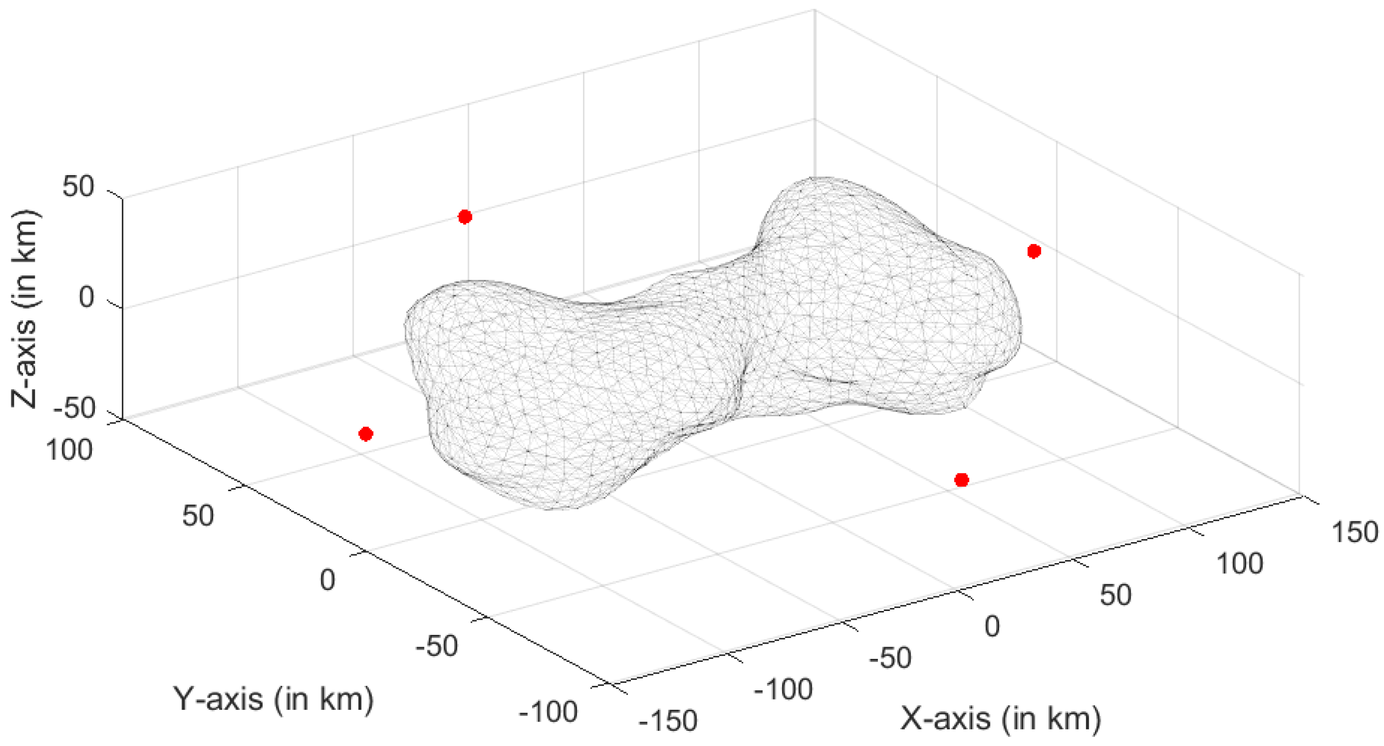
The position of Kleopatra’s four outside equilibrium points was obtained using a particle swarm optimization [46] followed by Newton’s iteration.

Table 1. Positions of equilibrium points of 216 Kleopatra in kilometers.

Equilibrium Point	x-Coordinate	y-Coordinate	z-Coordinate
1	143.12 km	3.08 km	0.34 km
2	−144.80 km	5.14 km	−1.44 km
3	−1.18 km	100.66 km	−0.93 km
4	1.29 km	−102.06 km	−0.13 km

shows the computed positions of the four equilibrium points in the body-fixed frame of Kleopatra. The accuracy of the equilibrium points obtained in this work is the same as obtained in previous literature studies on the computation of equilibrium points of Kleopatra (see [34,40] for the computation of equilibrium points of Kleopatra using symmetrical techniques). Hence, particle swarm optimization is a reliable technique to find initial locations of equilibrium points in the gravitational field of asteroids that are asymmetrical with respect to the equator. Figure 1 shows the position of the four outside equilibrium points in the body-fixed frame of Kleopatra. Interior equilibrium points are important in the study of the internal structural stability of an asteroid. In this paper, equilibrium points were computed in order to obtain small-amplitude periodic orbits around them. Interior equilibrium points would have these small-amplitude periodic orbits lying completely inside the body. Hence, interior equilibrium points are not relevant to the study of this paper. Readers can refer to [40] for information on the computation of equilibrium points inside Kleopatra. Specifically, for Kleopatra, there are three interior equilibrium points [40].

The stability of the equilibrium points was obtained by computing the eigenvalues of the system matrix of the variational equation (see Equation (6)). The pattern of the eigenvalues of the system matrix observed is studied in the literature [40]. It can be seen from

Table 2. Eigenvalues of Jacobian of vector field evaluated at equilibrium points of 216 Kleopatra.

Equilibrium Point	Eigenvalues
1	$\pm 7.3032$, $\pm 8.1884j$, $\pm 8.077j$
2	$\pm 8.1152$, $\pm 8.9717j$, $\pm 8.02j$
3	$3.9139\pm 5.9390j$, $-3.9139\pm 5.9390j$, $\pm 6.2489j$
4	$3.8934\pm 5.8917j$, $-3.8934\pm 5.8917j$, $\pm 6.3127j$

that small-amplitude periodic orbits exist in the center subspaces of equilibrium points because the Jacobian of the vector field of all the four equilibrium points of Kleopatra has at least one pair of purely imaginary eigenvalues. The center subspace of the first equilibrium point corresponding to the eigenvalue pair $\pm 8.077j$ was used for the computation of the vertical orbit family. The small-amplitude periodic orbits in the center subspace corresponding to $\pm 8.077j$ were continued to obtain the V1 family.

7.2. Period-Multiplying Orbits

7.2.1. V1 Family

The V1 family is the vertical periodic orbit family obtained from the continuation of the vertical small-amplitude periodic orbits close to the first equilibrium point (equilibrium point 1 of Kleopatra). The periodic orbit members of the V1 family eventually intersect with the surface of the asteroid as the continuation progresses. The continuation of the V1 family was stopped once a periodic orbit member collided with the surface of the asteroid during continuation. This part of the V1 family is taken as the parent family from which period-multiplying bifurcations are sought.

The eigenvalues of the monodromy matrices of the members along the parent family were of the form $\{\sigma ,{\displaystyle \frac{1}{\sigma }},1,1,v\pm nj\}$ with $v^1+n^2=1$, $\sigma \in \mathbb{R}$ and $0.58\le v\le 1$. For the V1 family, $\sigma$ was found to be of the order of $\mathcal{O}\left({10}^2\right)$ to $\mathcal{O}\left({10}^3\right)$. The eigenvalue $\sigma$ is called the unstable floquet multiplier of the periodic orbit. The time period of the members along the parent family lie in the range $[0.78T_h,0.94T_h]$, where $T_h$ is the rotational period of the asteroid. Hence, no resonant periodic orbits (periodic orbits whose periods are integer multiples of the rotational period of the asteroid) exist in the V1 family.

Period-multiplying bifurcations along the parent family were located by monitoring the unit circle eigenvalues $v\pm nj$ of the monodromy matrix of the periodic orbit members. The eigenvalues of the monodromy matrix on the unit circle were checked for the satisfaction of the conditions of Theorem 3. No period-multiplying bifurcations with an integer multiplying factor of six or less were present along the parent family. Multiple period-multiplying bifurcations with integer factors of greater than seven were located along the parent family.

Among the located period-multiplying bifurcations, one period 7- and one period 17-multiplying bifurcation were chosen for computation. Figure 2 shows the parent V1 family. Figure 3 shows the same parent V1 family from a different viewing angle. The different color lines in Figure 2 and Figure 3 indicate the different periodic orbit members of the V1 family. It can be seen from the viewing angle of Figure 3 that the V1 family starts as an elliptical orbit around the first equilibrium point and grows to a figure eight orbit covering a much larger region around the asteroid.

7.2.2. Period 7-Multiplying Bifurcation

One period 7 bifurcation was located along the parent V1 family. Since seven is a prime number, all the complex seventh roots of unity satisfy the conditions of Theorem 3. However, all the unit circle eigenvalues of the monodromy matrix of periodic orbit members of the parent V1 family were found to be on the right half of the complex plane. Only one pair of the seventh root of unity has a positive real part ($0.6235\pm 0.7818j$). A periodic orbit member with this specific unit circle eigenvalue was located along the V1 parent family.

Fixed branch-switching was performed to switch to the period 7 branch that intersects with the parent family at this bifurcating member. The Legendre–Gauss collocation scheme was used for branch-switching and the subsequent continuation of the period 7 branch. A uniform time grid with a step size of ${\displaystyle \frac{1}{150}}$ on the interval $[0,1]$ was used. The degree of the Legendre basis polynomials used on each interval was 24. To ensure a smooth branch switch, it is important to avoid any false solutions that may arise due to the numerical method being used. In this study, spurious solutions were avoided by increasing the degree of the Legendre basis polynomials used to obtain the true converged solution.

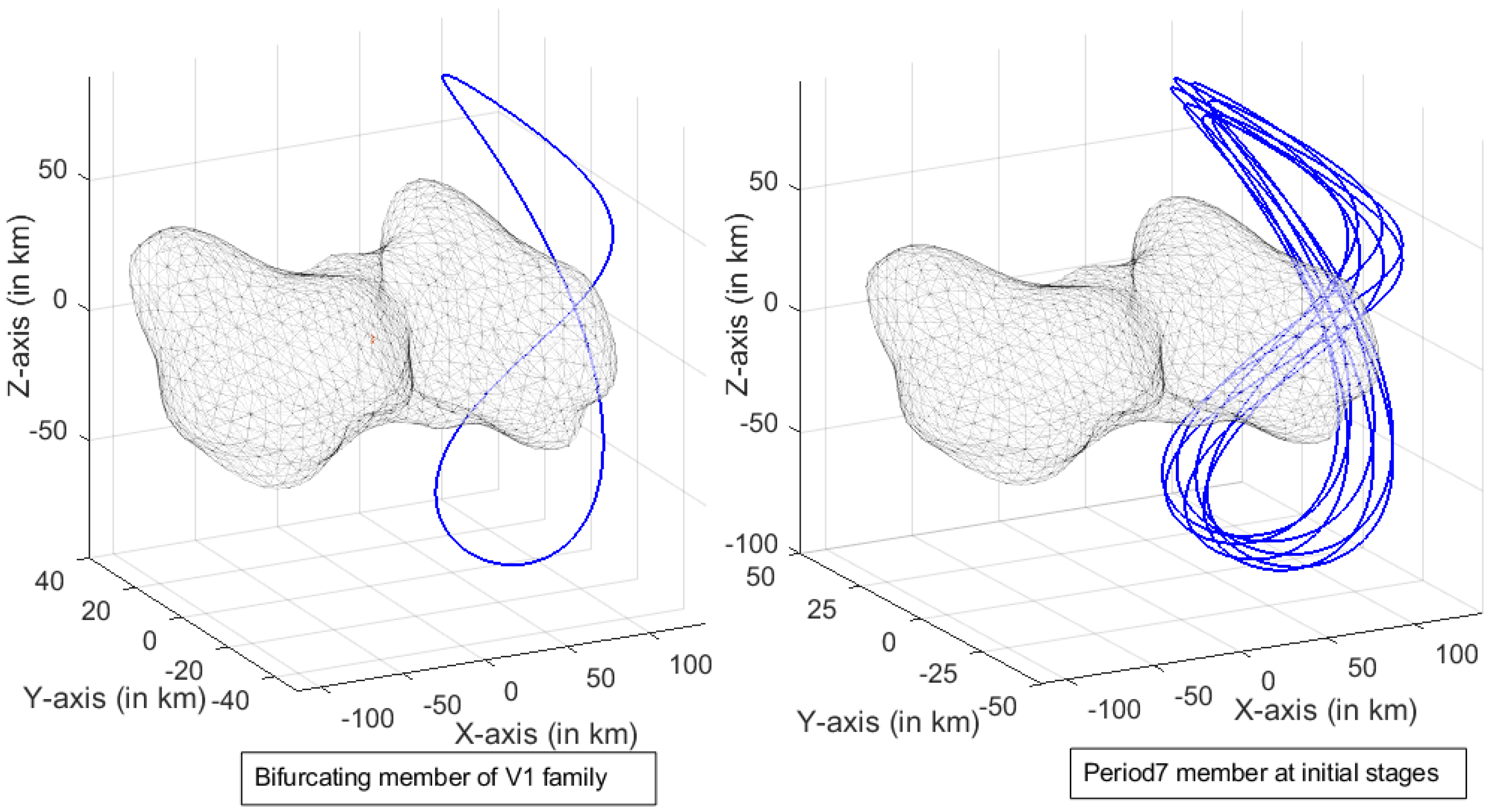
Like its parent V1 family, the period 7-multiplying branch also intersected with the surface of the asteroid as the continuation progressed. The continuation was stopped when the members started colliding with the asteroid’s surface. Figure 4 shows a member of the period 7-multiplying branch at intermediate stages of continuation in comparison with the bifurcating member of the V1 family. Figure 5 shows a member of the period 7-multiplying branch at final stages of continuation.

At the beginning of the continuation of the period-multiplying branch, the members looked almost identical to the respective parent branches. As the continuation progressed, the members gained additional revolutions over the figure eight shape of the bifurcating parent family member. At the initial stages of continuation, the members of the period 7 branch maintained the figure eight shape of the bifurcating parent family member. From Figure 4, it can seen that the gap between the revolutions increases, making the figure eight shape noticeably thicker. It can be seen from Figure 5 that at final stages of continuation, the shapes of the members no longer have the figure eight shape but still resemble the shape of the parent family. Throughout the continuation of the period 7 branch, a constant amplitude along the z-axis and y-axis was observed to be maintained, but the amplitude along the x-axis increased.

The shooting method did not work for the computation of the period 7-multiplying branch. After obtaining a member of the period 7 branch at the final stages of continuation (Figure 5) using the Legendre–Gauss collocation method, the reproduction of results was attempted using the multiple-shooting method on the same time grid (uniform time grid with step size of ${\displaystyle \frac{1}{150}}$ on the interval $[0,1]$) used in the Legendre–Gauss collocation. The multiple-shooting method applied to obtain the period 7 orbit at the final stage of continuation did not converge even when a finer uniform time grid was used. The multiple-shooting algorithm was stopped midway during the iteration at the minimum residual, and the trajectory was obtained (Figure 6). Figure 6 shows that such a reproduction fails, as the result is neither periodic nor roughly accurate to the period 7 branch member. The multiple-shooting method produces an erroneous solution that eventually collides with the asteroid’s surface, whereas the actual correct solution does not collide with the asteroid. This shows the unreliable nature of studying long-duration trajectories around asteroids using shooting methods. It can be inferred from Equation (15) that periodic orbit members of the period-multiplying branch are more sensitive to disturbances in initial conditions than periodic orbit members of the parent branch. This is because the floquet multipliers (eigenvalues of the monodromy matrix) of the periodic orbit are the measure of the sensitivity of the periodic orbit with respect to the initial conditions [32]. The unstable floquet multiplier of the period 7 bifurcating member of the parent vertical periodic orbit family was found to be of $\mathcal{O}\left({10}^2\right)$. Hence, from Equation (15), the floquet multiplers of the period 7-multiplying branch members are of the order $\mathcal{O}\left({10}^{14}\right)$. Pellegrini and Russell proposed that the computational difficulties observed during shooting methods are because of the usage of variable step numerical integrators to compute periodic orbits with large floquet multipliers [32]. They further showed that the fixed-step integration of Equation (17) overcomes the problems encountered in shooting methods. Several successful applications of the shooting methods using fixed-step integration have been demonstrated in the computation of periodic orbits having floquet multipliers of the order $\mathcal{O}\left({10}^6\right)$ in the Earth–Moon system. This work used the fixed-step integration of Equation (17) for the multiple-shooting method to compute period-multiplying bifurcations of periodic orbit families in asteroid environments. Computational difficulties were still observed when the multiple-shooting method with fixed-step integration was applied to obtain period-multiplying bifurcations around asteroids, as explained above. Extra care must be taken even if the problem of studying long-duration trajectories around asteroids is recast into a boundary value problem (as is performed in this paper, by computing periodic orbits through a two-point boundary value problem as opposed to grid-search methods used in the literature [19]). In this work, shooting methods could not obtain period-multiplying branches of periodic orbit families around asteroids. The boundary value problem was solved successfully by using the Legendre–Gauss collocation method. Hence, the Legendre–Gauss collocation method is proposed as an alternative to study long-duration orbits around asteroids when computational difficulties are encountered while using shooting methods to obtain long-duration orbits around asteroids.

7.2.3. Period 17-Multiplying Bifurcation

Two period 17 bifurcations were located along the parent V1 family. Of the 17 roots, only 4 have positive real parts ($0.7390\pm 0.6737j$ and $0.9325\pm 0.3612j$). Two periodic orbit members with these specific unit circle eigenvalues were located along the V1 parent family. The periodic orbit member whose monodromy matrix has an eigenvalue pair of $0.7390\pm 0.6737j$ was chosen to compute the period-multiplying branch. The floquet multiplier of the bifurcating periodic orbit member of the parent V1 family was found to be of the order of $\mathcal{O}\left({10}^2\right)$.

A uniform time grid with a step size of ${\displaystyle \frac{1}{240}}$ on the interval $[0,1]$ was used. The degree of the Legendre basis polynomials on each interval was 32.

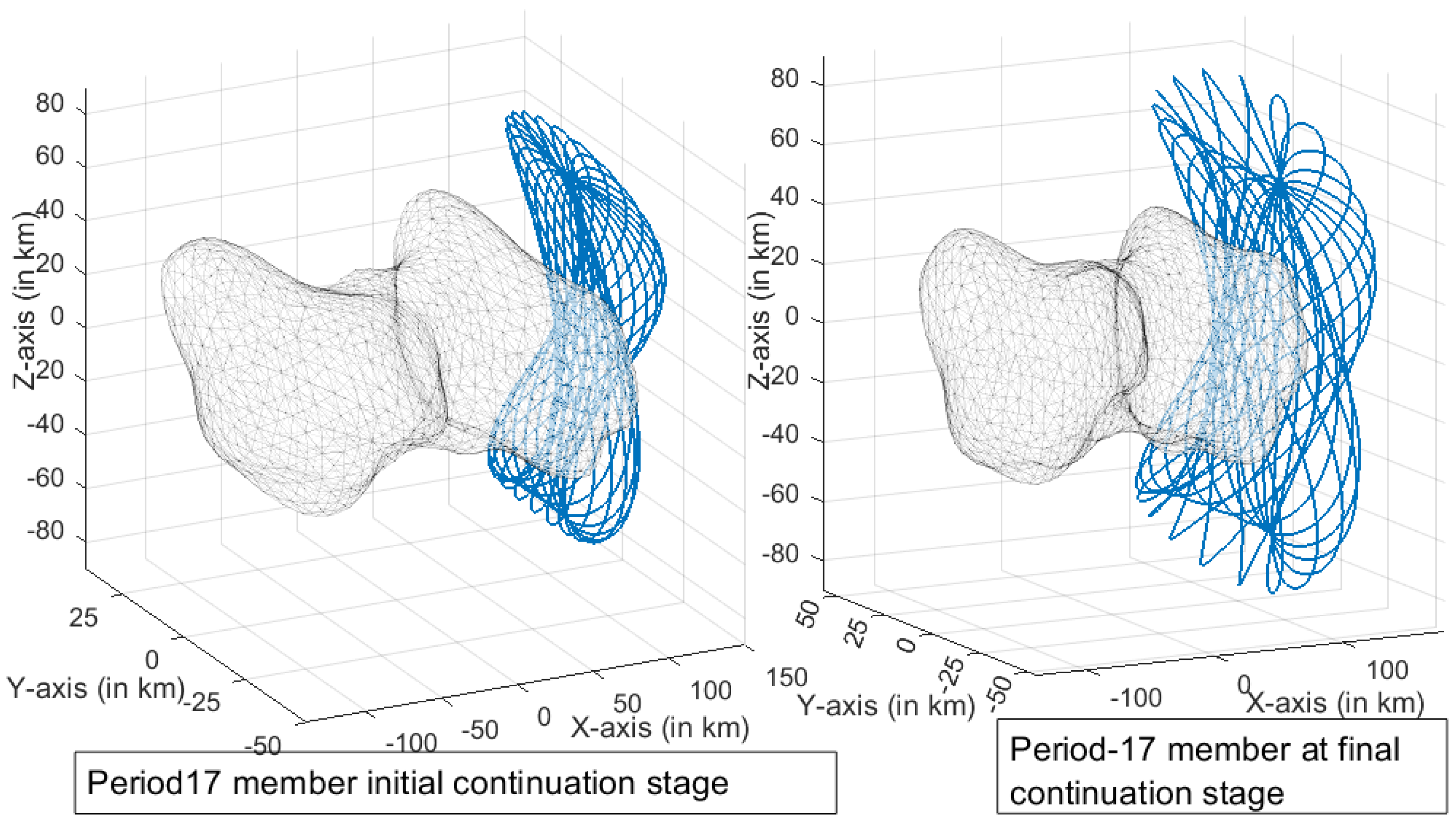
The period 17-multiplying branch collided with the surface of the asteroid as the continuation progressed. The continuation was stopped at the collision. Figure 7 shows a member of the period 17 branch during the initial stages of continuation. The initial members of the period 17 branch were identical to the parent family. Figure 7 shows that at the initial stages of continuation, the period 17 branch members maintained the figure eight shape of the parent family members; this behavior was similar to the period 7 branch.

On the other hand, at the intermediate and final stages of continuation, the period 17 branch exhibited different behavior from the period 7 branch. Figure 8 shows the evolution of the period 17-multiplying branch as the continuation progresses from intermediate to final stages. The intermediate members of the period 17 branch do not have a figure eight shape. Moreover, the shape of the period 17 branch does not resemble the shape of the parent family members. At the final stages of continuation, the y-amplitude of the period 17 branch members increased in addition to the increase in x-amplitudes. The z-amplitude was constant as the continuation progressed.

8. Conclusions

This paper presented a systematic approach for computing high-period periodic orbits around asteroids. The methodology involved first computing a parent periodic orbit family by computing a small-amplitude periodic orbit about an equilibrium point of the asteroid and then using the continuation technique to obtain the other periodic orbits, thus obtaining a family of periodic orbits. After identifying the locations at which the parent family bifurcates to give rise to a period-multiplying periodic orbit family, the members of the period-multiplying periodic orbit family were computed. This is in contrast with the grid search method used in the literature.

The single-shooting method using high-fidelity integrators like ode78 or ode89 was used to obtain the parent family. A collocation-based scheme was required to compute the members of the period-multiplying branch, as even multiple-shooting using ode78 or ode89 failed to give a converged solution. The limitation of shooting methods in computing high-period periodic orbits also points to the inappropriateness of using standard solvers like ode78 or ode89 for simulating long-duration trajectories about asteroids.

As a demonstration of the methodology presented, period 7 and period 17 periodic orbit families about the asteroid Kleopatra were computed. Upon continuation, the period 17 orbits that bifurcated from the parent family resulted in an orbit that is very different from the orbit of the parent family, pointing to its potential use in certain missions that require orbits with certain coverage. While a stability analysis of the computed high-period orbits remains as future work, the potential for identifying high-period orbits that are more stable compared to the parent family opens exciting avenues for further research.

References

- Prockter, L.; Murchie, S.; Cheng, A.; Krimigis, S.; Farquhar, R.; Santo, A.; Trombka, J. The NEAR shoemaker mission to asteroid 433 Eros. Acta Astronaut. 2002, 51, 491–500. [Google Scholar] [CrossRef]
- Kawaguchi, J.; Fujiwara, A.; Uesugi, T. Hayabusa—Its technology and science accomplishment summary and Hayabusa-2. Acta Astronaut. 2008, 62, 639–647. [Google Scholar] [CrossRef]
- Huang, J.; Ji, J.; Ye, P.; Wang, X.; Yan, J.; Meng, L.; Wang, S.; Li, C.; Li, Y.; Qiao, D.; et al. The ginger-shaped asteroid 4179 Toutatis: New observations from a successful flyby of Chang’e-2. Sci. Rep. 2013, 3, 3411. [Google Scholar] [CrossRef] [PubMed]
- Glassmeier, K.H.; Boehnhardt, H.; Koschny, D.; Kührt, E.; Richter, I. The Rosetta mission: Flying towards the origin of the solar system. Space Sci. Rev. 2007, 128, 1–21. [Google Scholar] [CrossRef]
- Lauretta, D.; Balram-Knutson, S.; Beshore, E.; Boynton, W.; Drouet d’Aubigny, C.; DellaGiustina, D.; Enos, H.; Golish, D.; Hergenrother, C.; Howell, E.; et al. OSIRIS-REx: Sample return from asteroid (101955) Bennu. Space Sci. Rev. 2017, 212, 925–984. [Google Scholar] [CrossRef]
- Watanabe, S.i.; Tsuda, Y.; Yoshikawa, M.; Tanaka, S.; Saiki, T.; Nakazawa, S. Hayabusa2 mission overview. Space Sci. Rev. 2017, 208, 3–16. [Google Scholar] [CrossRef]
- Veverka, J.; Farquhar, B.; Robinson, M.; Thomas, P.; Murchie, S.; Harch, A.; Antreasian, P.G.; Chesley, S.R.; Miller, J.K.; Owen, W.M.; et al. The landing of the NEAR-Shoemaker spacecraft on asteroid 433 Eros. Nature 2001, 413, 390–393. [Google Scholar] [CrossRef] [PubMed]
- Herrera-Sucarrat, E.; Palmer, P.L.; Roberts, R.M. Asteroid observation and landing trajectories using invariant manifolds. J. Guid. Control Dyn. 2014, 37, 907–920. [Google Scholar] [CrossRef]
- Kohout, T.; Näsilä, A.; Tikka, T.; Granvik, M.; Kestilä, A.; Penttilä, A.; Kuhno, J.; Muinonen, K.; Viherkanto, K.; Kallio, E. Feasibility of asteroid exploration using CubeSats—ASPECT case study. Adv. Space Res. 2018, 62, 2239–2244. [Google Scholar] [CrossRef]
- Fujiwara, A.; Kawaguchi, J.; Yeomans, D.K.; Abe, M.; Mukai, T.; Okada, T.; Saito, J.; Yano, H.; Yoshikawa, M.; Scheeres, D.J.; et al. The rubble-pile asteroid Itokawa as observed by Hayabusa. Science 2006, 312, 1330–1334. [Google Scholar] [CrossRef]
- Ostro, S.J.; Scott, R.; Hudson; Nolan, M.C.; Margot, J.L.; Scheeres, D.J.; Campbell, D.B.; Magri, C.; Giorgini, J.D.; Yeomans, D.K. Radar observations of asteroid 216 Kleopatra. Science 2000, 288, 836–839. [Google Scholar] [CrossRef]
- Kaasalainen, M.; Torppa, J.; Muinonen, K. Optimization methods for asteroid lightcurve inversion: II. The complete inverse problem. Icarus 2001, 153, 37–51. [Google Scholar] [CrossRef]
- Werner, R.A.; Scheeres, D.J. Exterior gravitation of a polyhedron derived and compared with harmonic and mascon gravitation representations of asteroid 4769 Castalia. Celest. Mech. Dyn. Astron. 1996, 65, 313–344. [Google Scholar] [CrossRef]
- Urevc, J.; Halilovič, M. Enhancing accuracy of Runge–Kutta-type collocation methods for solving ODEs. Mathematics 2021, 9, 174. [Google Scholar] [CrossRef]
- Muñoz-Almaraz, F.J.; Freire, E.; Galán, J.; Doedel, E.; Vanderbauwhede, A. Continuation of periodic orbits in conservative and Hamiltonian systems. Phys. D Nonlinear Phenom. 2003, 181, 1–38. [Google Scholar] [CrossRef]
- Lara, M.; Peláez, J. On the numerical continuation of periodic orbits-an intrinsic, 3-dimensional, differential, predictor-corrector algorithm. Astron. Astrophys. 2002, 389, 692–701. [Google Scholar] [CrossRef]
- Pal, A.K.; Abouelmagd, E.I.; Guirao, J.L.G.; Brzeziński, D.W. Periodic solutions of nonlinear relative motion satellites. Symmetry 2021, 13, 595. [Google Scholar] [CrossRef]
- Zeng, X.; Liu, X. Searching for time optimal periodic orbits near irregularly shaped asteroids by using an indirect method. IEEE Trans. Aerosp. Electron. Syst. 2017, 53, 1221–1229. [Google Scholar] [CrossRef]
- Yu, Y.; Baoyin, H. Generating families of 3D periodic orbits about asteroids. MNRAS 2012, 427, 872–881. [Google Scholar] [CrossRef]
- Jiang, M.; Ma, Q. The dynamical environment of the primary in the triple asteroid (45) Eugenia. Open Astron. 2020, 29, 59–71. [Google Scholar] [CrossRef]
- Jiang, Y. Dynamical environment in the triple asteroid system 87 Sylvia. Astrophys. Space Sci. 2019, 364, 60. [Google Scholar] [CrossRef]
- Jiang, Y.; Li, H. Equilibria and orbits in the dynamical environment of asteroid 22 Kalliope. Open Astron. 2019, 28, 154–164. [Google Scholar] [CrossRef]
- Zhang, Y.; Zeng, X.; Liu, X. Study on periodic orbits around the dipole segment model for dumbbell-shaped asteroids. Sci. China Technol. Sci. 2018, 61, 819–829. [Google Scholar] [CrossRef]
- Shang, H.; Wu, X.; Ren, Y.; Shan, J. An efficient algorithm for global periodic orbits generation near irregular-shaped asteroids. Commun. Nonlinear Sci. Numer. Simul. 2017, 48, 550–568. [Google Scholar] [CrossRef]
- Jiang, Y.; Baoyin, H. Periodic orbit families in the gravitational field of irregular-shaped bodies. Astron. J. 2016, 152, 137. [Google Scholar] [CrossRef]
- Liu, Y.; Jiang, Y.; Li, H.; Liu, Y.; Jiang, Y.; Li, H. Bifurcations of periodic orbits in the gravitational field of irregular bodies: Applications to Bennu and Steins. Aerospace 2022, 9, 151. [Google Scholar] [CrossRef]
- Jiang, Y.; Yu, Y.; Baoyin, H. Topological classifications and bifurcations of periodic orbits in the potential field of highly irregular-shaped celestial bodies. Nonlinear Dyn. 2015, 81, 119–140. [Google Scholar] [CrossRef]
- Ni, Y.; Jiang, Y.; Baoyin, H. Multiple bifurcations in the periodic orbit around Eros. Astrophys. Space Sci. 2016, 361, 170. [Google Scholar] [CrossRef]
- Jiang, Y.; Baoyin, H. Periodic orbits related to the equilibrium points in the potential of irregular-shaped minor celestial bodies. Results Phys. 2019, 12, 368–374. [Google Scholar] [CrossRef]
- Vanderbauwhede, A. Branching of periodic orbits in Hamiltonian and reversible systems. In Equadiff; Masaryk University: Brno, Czech Republic, 1998; Volume 9, p. 169. [Google Scholar]
- Li, Q.; Tao, Y.; Jiang, F. Orbital stability and invariant manifolds on distant retrograde orbits around Ganymede and nearby higher-period orbits. Aerospace 2022, 9, 454. [Google Scholar] [CrossRef]
- Pellegrini, E.; Russell, R.P. On the computation and accuracy of trajectory state transition matrices. J. Guid. Control Dyn. 2016, 39, 2485–2499. [Google Scholar] [CrossRef]
- Brown, G.M.; Scheeres, D.J. Analyzing the structure of periodic orbit families that exist around asteroid (101955) Bennu. Celest. Mech. Dyn. Astron. 2023, 135, 52. [Google Scholar] [CrossRef]
- Jiang, Y. Equilibrium points and periodic orbits in the vicinity of asteroids with an application to 216 Kleopatra. Earth Moon Planets 2015, 115, 31–44. [Google Scholar] [CrossRef]
- Jiang, Y.; Ni, Y.; Baoyin, H.; Li, J.; Liu, Y. Asteroids and their mathematical methods. Mathematics 2022, 10, 2897. [Google Scholar] [CrossRef]
- Zeng, X.; Jiang, F.; Li, J.; Baoyin, H. Study on the connection between the rotating mass dipole and natural elongated bodies. Astrophys. Space Sci. 2015, 356, 29–42. [Google Scholar] [CrossRef]
- Guo, B.Y.; Wang, Z.Q. Legendre–Gauss collocation methods for ordinary differential equations. Adv. Comput. Math. 2009, 30, 249–280. [Google Scholar] [CrossRef]
- Zeng, X.; Zhang, Y.; Yu, Y.; Liu, X. The dipole segment model for axisymmetrical elongated asteroids. Astron. J. 2018, 155, 85. [Google Scholar] [CrossRef]
- Wen, T.; Zeng, X. Equilibrium points of heterogeneous small body in finite element method. Mon. Not. R. Astron. Soc. 2023, 519, 6077–6087. [Google Scholar] [CrossRef]
- Wang, X.; Jiang, Y.; Gong, S. Analysis of the potential field and equilibrium points of irregular-shaped minor celestial bodies. Astrophys. Space Sci. 2014, 353, 105–121. [Google Scholar] [CrossRef]
- Wang, D.; Tan, D.; Liu, L. Particle swarm optimization algorithm: An overview. Soft Comput. 2018, 22, 387–408. [Google Scholar] [CrossRef]
- Poincaré, H. The Three-Body Problem and the Equations of Dynamics: Poincaré’s Foundational Work on Dynamical Systems Theory; Springer: Berlin/Heidelberg, Germany, 2017. [Google Scholar]
- Lust, K. Improved numerical Floquet multipliers. Int. J. Bifurc. Chaos 2001, 11, 2389–2410. [Google Scholar] [CrossRef]
- Liu, F.; Hager, W.W.; Rao, A.V. Adaptive mesh refinement method for optimal control using nonsmoothness detection and mesh size reduction. J. Frankl. Inst. 2015, 352, 4081–4106. [Google Scholar] [CrossRef]
- Calleja, R.C.; Doedel, E.J.; Humphries, A.R.; Lemus-Rodríguez, A.; Oldeman, E. Boundary-value problem formulations for computing invariant manifolds and connecting orbits in the circular restricted three body problem. Celest. Mech. Dyn. Astron. 2012, 114, 77–106. [Google Scholar] [CrossRef]
- The MathWorks, Inc. Optimization Toolbox; MATLAB R2021b; The MathWorks, Inc.: Natick, MA, USA, 2022. [Google Scholar]
Figure 1.
Position of equilibrium points in the body-fixed frame.
Figure 2.
V1 family of periodic orbits.
Figure 3.
V1 family of periodic orbits viewed from Y-axis.
Figure 4.
A member of the period 7 branch at the intermediate stage of continuation.
Figure 5.
A member of the period 7 branch at the final stage of continuation obtained through the collocation method.
Figure 6.
A member of the period 7 branch at the final stage of continuation obtained through the shooting method.
Figure 7.
A member of the period 17 branch during the initial stages of continuation.
Figure 8.
Evolution of the period 17 branch.