
Analysis of Radio Frequency Blackout for a Blunt-Body Capsule in Atmospheric Reentry Missions

Abstract
:
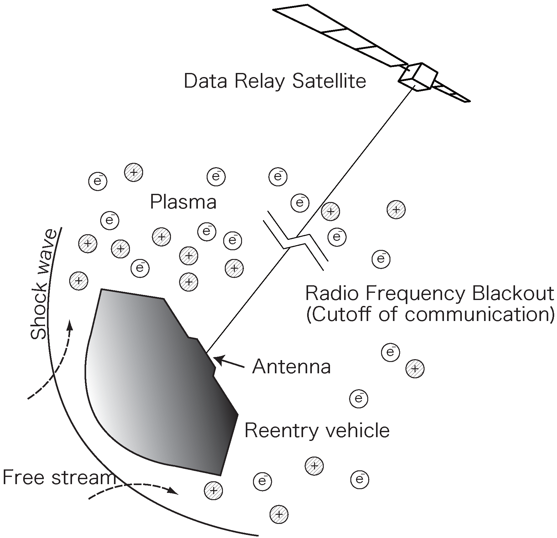
1. Introduction

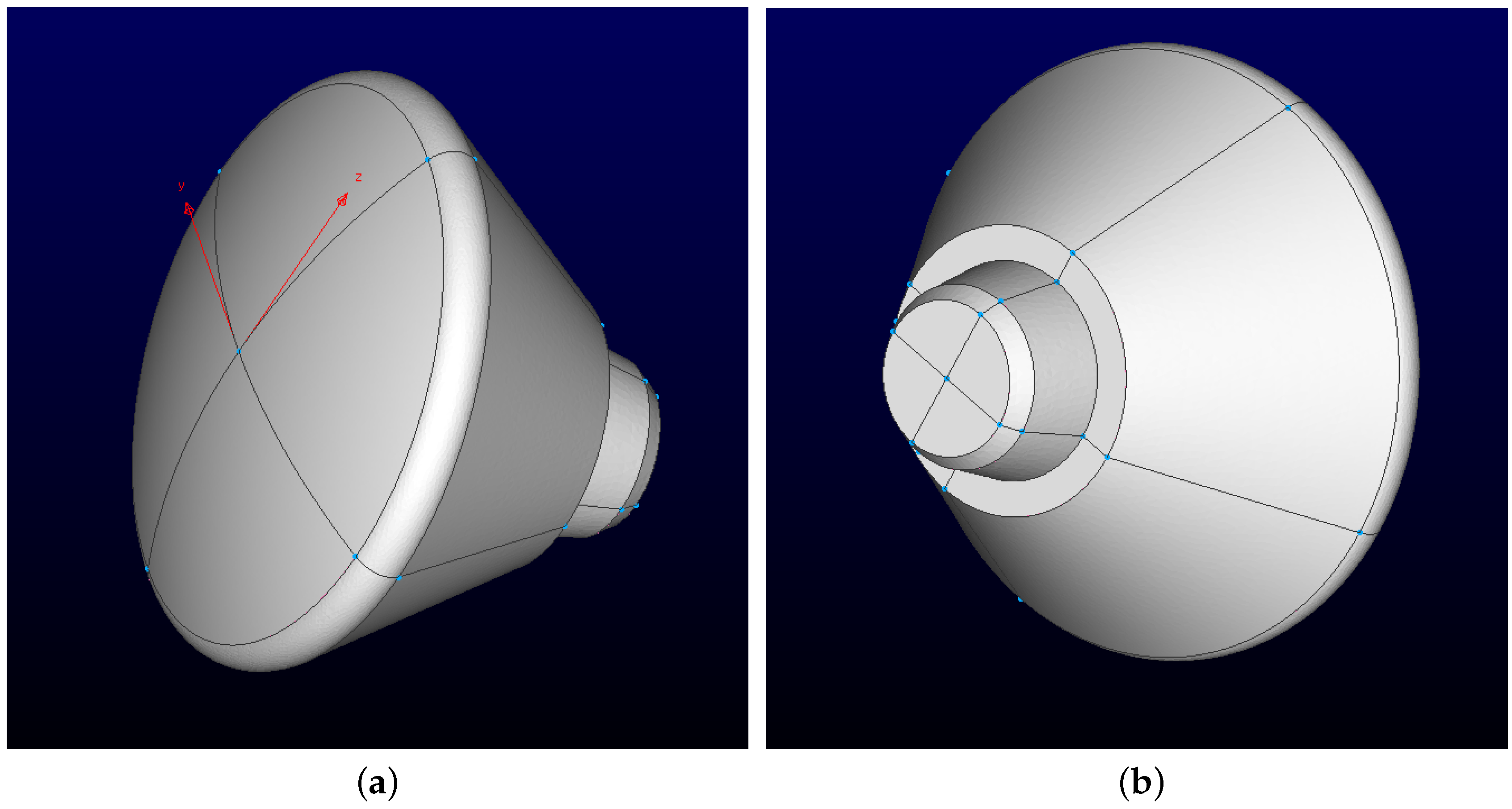
2. Reentry Vehicle


3. Flow Field Modeling
3.1. Governing Equation
3.2. Transport Properties
3.3. Chemical Reactions
3.4. Internal Energy Exchange
3.5. Implementation
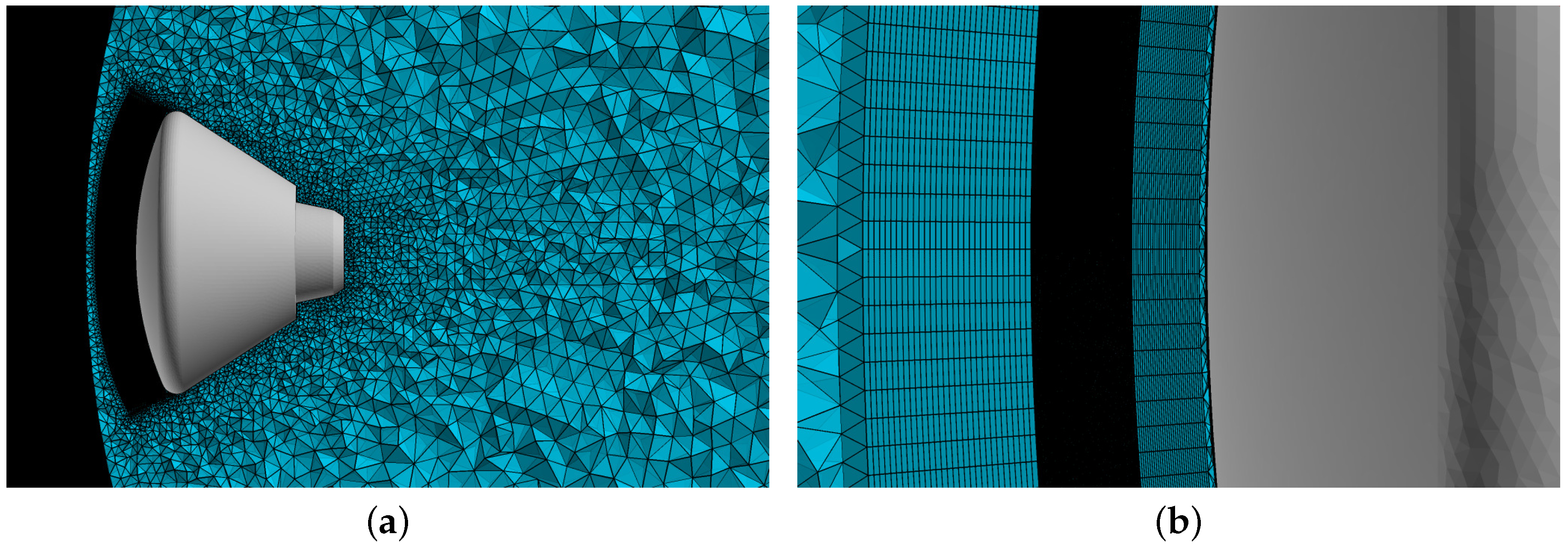
3.6. Computational and Boundary Conditions

| Altitude, km | Density, kg/m | Temperature, K | Velocity, m/s | AOA, Degree |
|---|---|---|---|---|
| 85.0 | 8.18 × 10 | 191.0 | 7577 | 20.0 |
| 80.0 | 1.85 × 10 | 195.8 | 7609 | 20.0 |
| 75.0 | 4.07 × 10 | 201.7 | 7593 | 19.2 |
| 70.0 | 8.83 × 10 | 210.9 | 7542 | 19.2 |
| 60.0 | 3.40 × 10 | 242.0 | 6105 | 19.4 |
| 50.0 | 1.15 × 10 | 265.3 | 4567 | 20.0 |


4. Electromagnetic Wave Modeling
4.1. Maxwell’s Equations
4.2. FD2TD Method
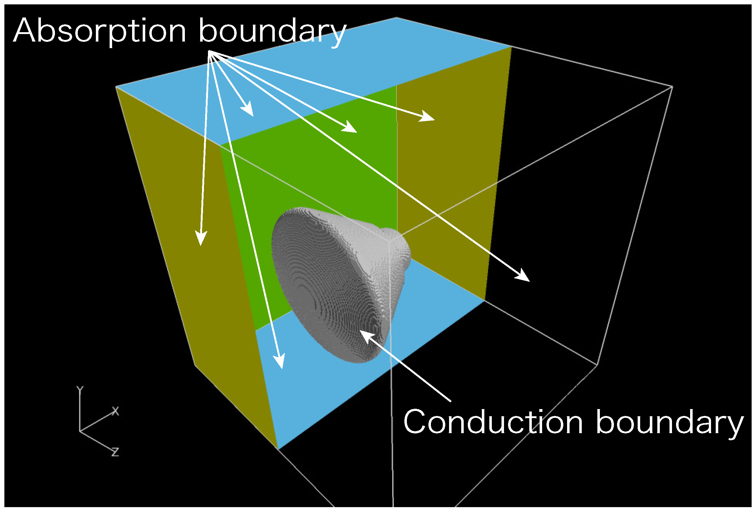
4.3. Computational Domain

5. Results and Discussion
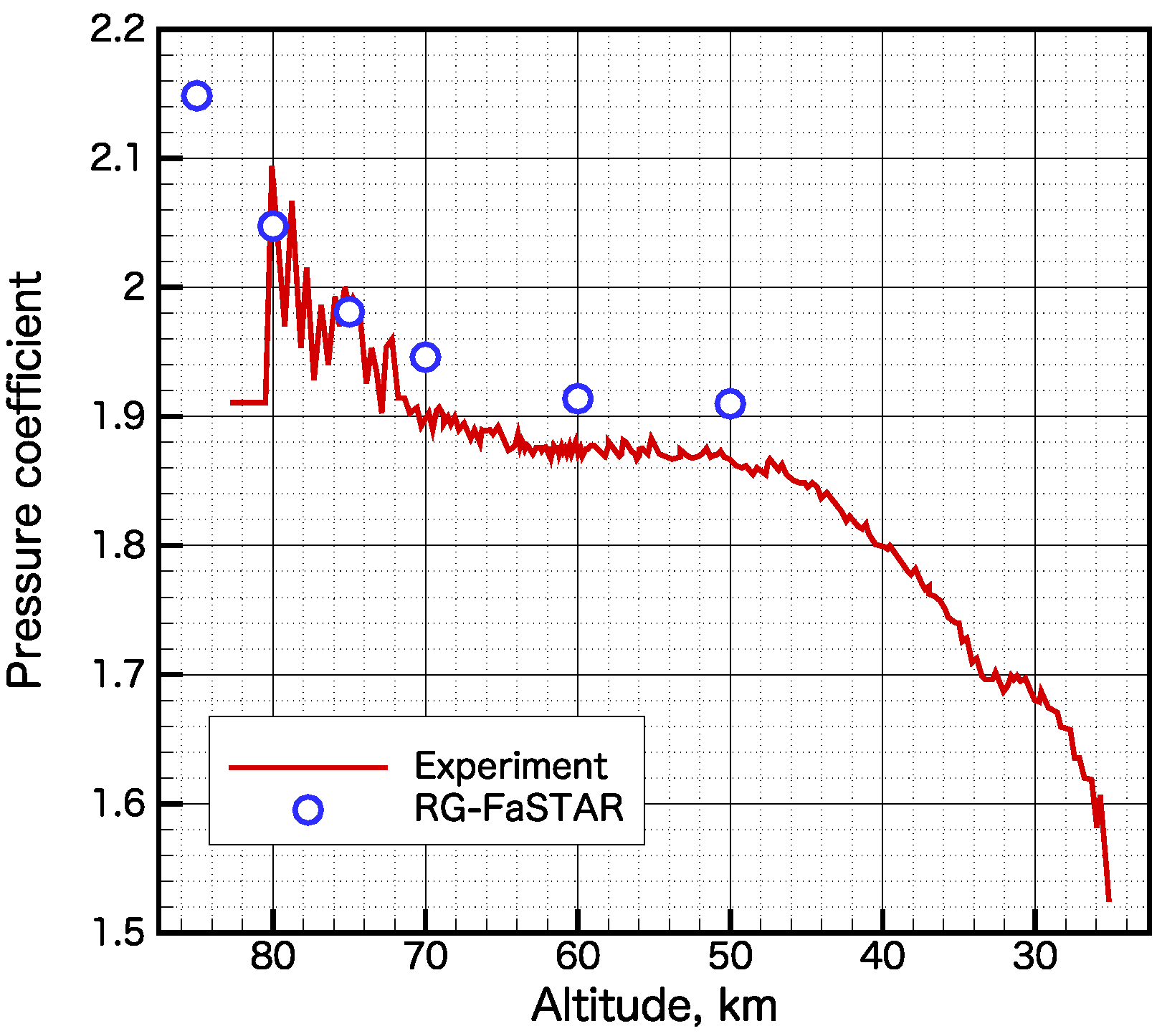
5.1. Stagnation Pressure

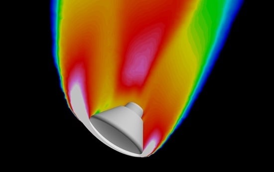
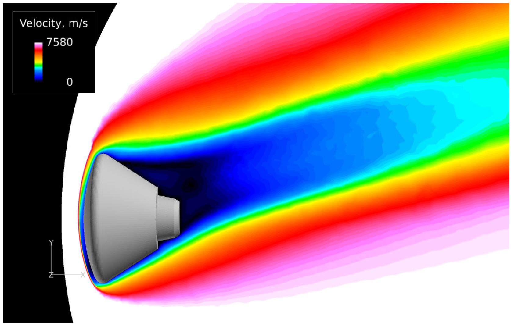
5.2. Plasma Flow Field


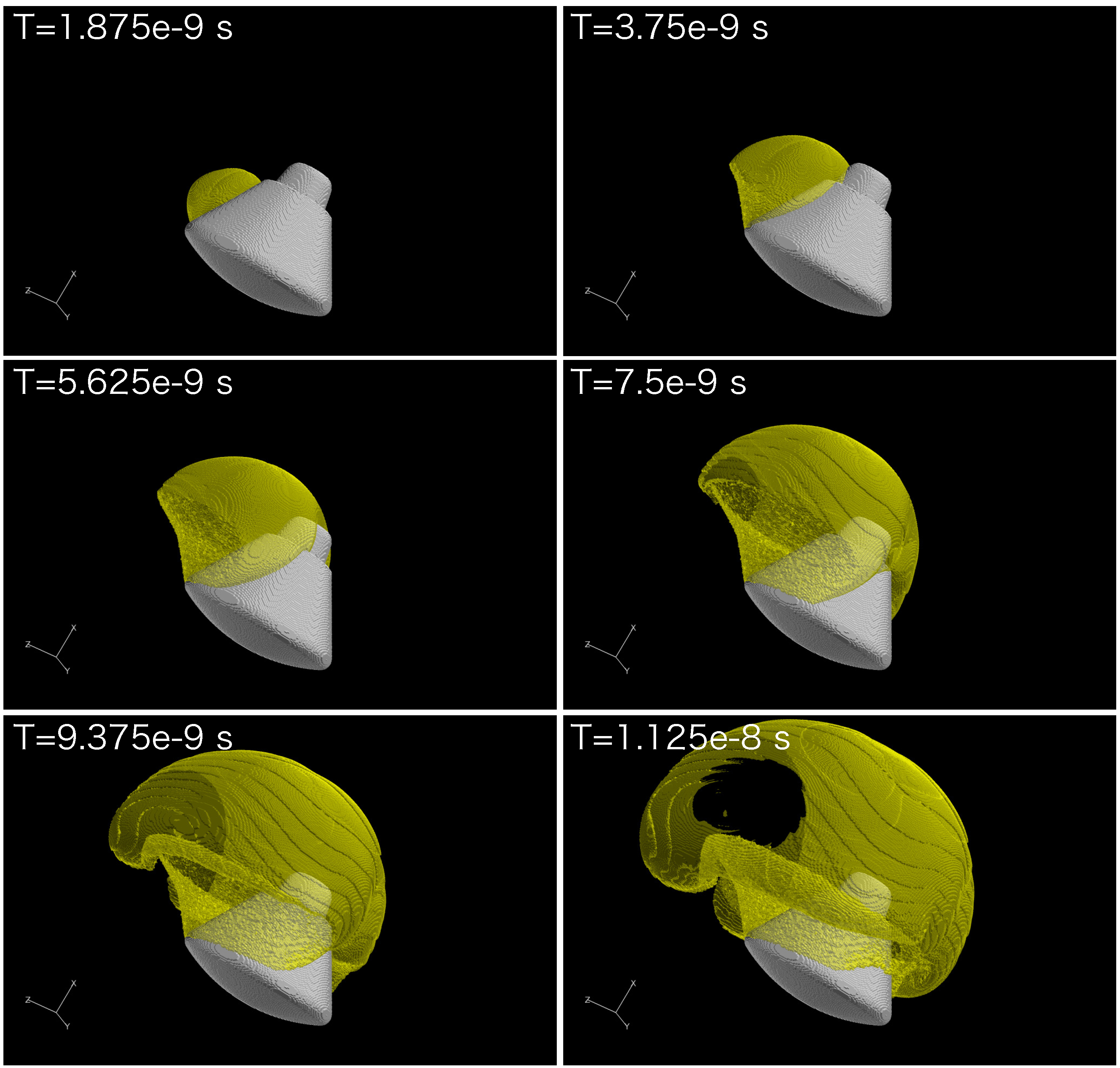
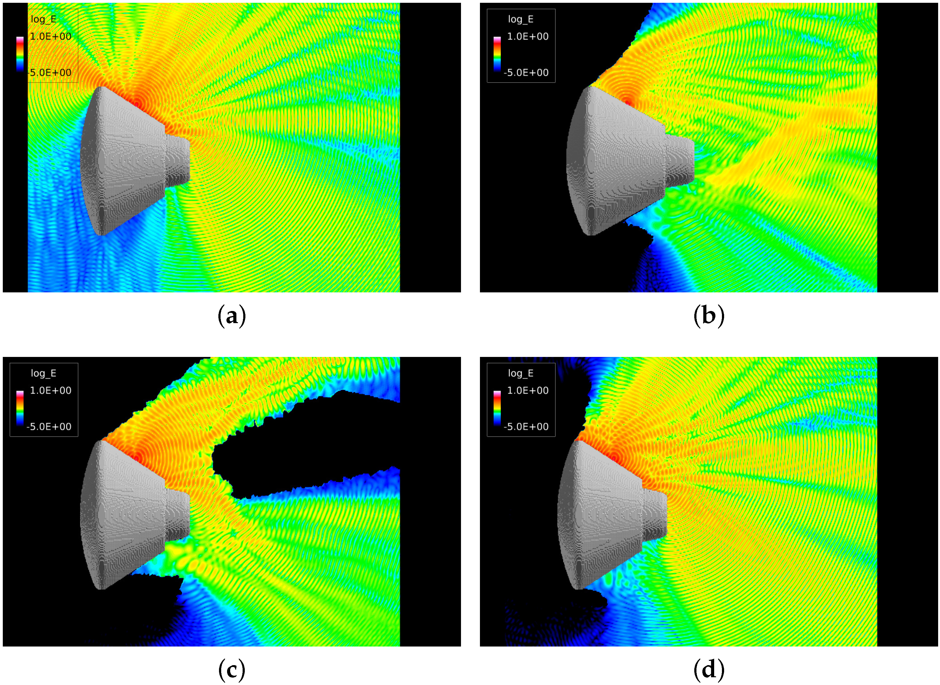
5.3. Electromagnetic Waves


6. Conclusions
Acknowledgments
Author Contributions
Conflicts of Interest
Abbreviations
| ARD | = Atmospheric reentry demonstrator |
| CFD | = Computational fluid dynamics |
| ESA | = European Space Agency |
| FD2TD | = Frequency-dependent finite-difference time-domain |
| FDTD | = Finite-difference time-domain |
| GPS | = Global Positioning System |
| JAXA | = Japan Aerospace Exploration Agency |
| LU-SGS | = Lower-upper symmetric Gauss–Seidel |
| MPI | = Message Passing Interface |
| MUSCL | = Monotonic upstream-centered scheme for interpolation of conservation laws |
| NAL | = National Aerospace Laboratory of Japan |
| NASA | = National Aeronautics and Space Administration |
| NASDA | = National Space Development Agency of Japan |
| OpenMP | = Open Multi-Processing |
| RAM | = Radio attenuation measurement |
| RF | = Radio frequency |
| TDRS | = Tracking and data relay satellite |
| = magnetic flux density vector, T | |
| D | = effective diffusion coefficient, m/s |
| = electric flux density vector, C/m | |
| e | = elementary charge, C |
| E | = internal energy J/m |
| = electric field vector, V/m | |
| = vector of advection/viscous flux | |
| = enthalpy of formation, J/kg | |
| = current density vector, A/m | |
| = magnetic field vector, A/m | |
| k | = Boltzmann constant, J/K |
| m | = mass, kg |
| n | = number density, 1/m |
| = number of molecules | |
| = number of chemical species | |
| p | = pressure, Pa |
| = vector of conservative variables | |
| R | = gas constant, J/(kg·K) |
| t | = time, s |
| T | = temperature, K |
| = velocity, m/s | |
| = vector of source terms | |
| = coordinate | |
| = relative permittivity | |
| = permittivity in free space, N/V | |
| Θ | = characteristic temperature, K |
| = permeability in free space, N/A | |
| ν | = collision frequency, Hz |
| ρ | = density, kg/m |
| σ | = conductivity, S/m |
| χ | = electric susceptibility |
| ω | = angular frequency, rad/s |
| = plasma angular frequency, rad/s | |
| Ω | = collision cross section, m |
| Subscripts | |
| = collision | |
| = electron | |
| = plasma | |
| = relative | |
| = rotation | |
| s | = species |
| = translation | |
| v | = viscous |
| = vibration | |
| ∞ | = freestream |
| Superscripts | |
| = ambipolar | |
| = equilibrium | |
| = time step | |
References
- Rybak, J.P.; Churchill, R.J. Progress in reentry communications. IEEE Trans. Aerosp. Elect. Syst. 1971, 7, 879–894. [Google Scholar] [CrossRef]
- Schroeder, L.C.; Russo, F.P. Flight Investigation and Analysis of Alleviation of Communications Blackout by Water Injection during Gemini 3 Reentry; NASA TM X-1521; NASA: Washington, DC, USA, 1968; pp. 1–56. [Google Scholar]
- Usui, H.; Matsumoto, H.; Yamashita, F.; Yamane, M.; Takenaka, S. Computer experiments on radio blackout of a reentry vehicle. In Proceedings of 6th Spacecraft Charging Technology Conference; Cooke, D.L., Ed.; Eurpean Space Agency: Paris, France, 2000; pp. 107–110. [Google Scholar]
- Kim, M.; Keidar, M.; Boyd, I.D. Analysis of an electromagnetic mitigation scheme for reetnry telemetry through plasma. J. Spacecr. Rocket. 2008, 45, 1223–1229. [Google Scholar] [CrossRef]
- Belov, I.F.; Borovoy, V.Y.; Gorelov, V.A.; Kireev, A.Y.; Korolev, A.S.; Stepanov, E.A. Investigation of remote antenna assembly for radio communication with reentry vehicle. J. Spacecr. Rocket. 2001, 38, 249–256. [Google Scholar] [CrossRef]
- Takahashi, Y.; Yamada, K.; Abe, T. Examination of radio frequency blackout for an inflatable vehicle during atmospheric reentry. J. Spacecr. Rocket. 2014, 51, 430–441. [Google Scholar] [CrossRef]
- Vecchi, G.; Sabbadini, M.; Maggiora, R.; Siciliano, A. Modelling of antenna radiation pattern of a re-entry vehicle in presence of plasma. In Antennas and Propagation Society International Symposium, 2004; IEEE: New York, NY, USA, 2004; Volume 1, pp. 181–184. [Google Scholar]
- Vecchi, G.; Vipiana, F.; Vasquez, J.A.T.; Visintin, M.; Milani, F.; Bandinelli, M.; Sabbadini, M. Reentry vehicles: Evaluation of plasma effects on RF propagation. In Proceedings of the TTC 2013, 6th ESA International Workshop on Tracking, Telemetry, and Command Systems for Space Applications, Darmstadt, Germany, 10–13 September 2013; pp. 1–8.
- Delfino, A. Modeling of the Antenna Radiation Pattern of a Re-Entry Space Vehicle in the Presence of Plasma. Master’s Thesis, University of Illinois at Chicago, Chicago, IL, USA, 2004. [Google Scholar]
- Yucel, A.C.; Gomez, L.J.; Liu, Y.; Bagci, H.; Michielssen, E. A FMM-FFT accelerated hybrid volume surface integral equation solver for electromagnetic analysis of re-entry space vehicles. In Radio Science Meeting (Joint with AP-S Symposium), 2014 USNC-URSI; IEEE: New York, NY, USA, 2014; p. 66. [Google Scholar]
- White, M.D. Simulation of communications through a weakly ionized plasma for a re-entry vehicle at Mach 23.9. In Antennas and Propagation Society International Symposium, 2005 IEEE; IEEE: New York, NY, USA, 2015; Volume 4, pp. 418–421. [Google Scholar]
- Kunz, K.S.; Luebbers, R.J. The Finite Difference Time Domain Method for Electromagnetics; CRC Press: Boca Raton, FL, USA, 1993. [Google Scholar]
- Kinefuchi, K.; Funaki, I.; Abe, T. Frequency-dependent fdtd simulation of the interaction of microwaves with rocket-plume. IEEE Trans. Antennas Propag. 2010, 58, 3282–3288. [Google Scholar] [CrossRef]
- Takahashi, Y.; Yamada, K.; Abe, T. Prediction performance of blackout and plasma attenuation in atmospheric reentry demonstrator mission. J. Spacecr. Rocket. 2014, 51, 1954–1964. [Google Scholar] [CrossRef]
- Takahashi, Y. Advanced validation of CFD-FDTD combined method using highly applicable solver for reentry blackout prediction. J. Phys. D 2016, 49, 015201. [Google Scholar] [CrossRef]
- Tran, P.; Paulat, J.C.; Boukhobza, P. Re-Entry Flight Experiments Lessons Learned—the Atmospheric Reentry Demonstrator Ard; Nato Report, RTO-EN-AVT-130-10; RTO: Neuilly-sur-Seine, France, 2007; pp. 101–146. [Google Scholar]
- Yos, J.M. Transport Properties of Nitrogen, Hydrogen Oxygen and Air to 30,000 K; TRAD-TM-63-7; AVCO Corp.: Greenwich, CT, USA, 1963. [Google Scholar]
- Hirschfelder, J.O.; Curtiss, C.F.; Bird, R.B. Molecular Theory of Gases and Liquids; Wiley: New York, NY, USA, 1954. [Google Scholar]
- Gupta, R.N.; Yos, J.M.; Thompson, R.A.; Lee, K.P. A Review of Reaction Rates and Thermodynamic and Transport Properties for an 11-Species Air Model for Chemical and Thermal Nonequilibrium Calculations to 30000 K; NASA RP-1232; NASA: Washington, DC, USA, 1990. [Google Scholar]
- Fertig, M.; Dohr, A.; Frühaufu, H.H. Transport Coefficients for High-Temperature Nonequilibrium Air Flows; AIAA Paper 98-2937; AIAA: Reston, VA, USA, 1998. [Google Scholar]
- Fertig, M.; Dohr, A.; Frühauf, H.H. Transport coefficients for high-temperature nonequilibrium air flows. J. Thermophys. Heat Transfer. 2001, 15, 148–156. [Google Scholar] [CrossRef]
- Curtiss, C.F.; Hirschfelder, J.O. Transport properties of multicomponent gas mixture. J. Chem. Phys. 1949, 17, 550–555. [Google Scholar] [CrossRef]
- Park, C. Assessment of a two-temperature kinetic model for dissociating and weakly ionizing nitrogen. J. Thermophys. Heat Transf. 1998, 2, 8–16. [Google Scholar] [CrossRef]
- Park, C. Nonequilibrium Hypersonic Aerothermodynamics; Wiley: New York, NY, USA, 1990. [Google Scholar]
- Parker, J.G. Rotational and vibrational relaxation in diatomic gases. Phys. Fluids 1959, 2, 449–462. [Google Scholar] [CrossRef]
- Millikan, R.C.; White, D.R. Systematics of vibrational relaxation. J. Chem. Phys. 1963, 39, 3209–3213. [Google Scholar] [CrossRef]
- Park, C. Problems of Rate Chemistry in the Flight Regimes of Aeroassisted Orbital Transfer Vehicles; AIAA Paper 84-1730; AIAA: Reston, VA, USA, 1984. [Google Scholar]
- Appleton, J.P.; Bray, K.N.C. The conservation equations for a nonequilibrium plasma. J. Fluid Mech. 1964, 20, 659–672. [Google Scholar] [CrossRef]
- Mitchner, M.; Kruger, C.H., Jr. Partially Ionized Gases; Wiley: New York, NY, USA, 1973. [Google Scholar]
- Gnoffo, P.A.; Gupta, R.N.; Shinn, J.L. Conservation Equations and Physical Models for Hypersonic Air Flows in Thermal and Chemical Nonequilibrium; NASA TP-2867; NASA: Washington, DC, USA, 1989. [Google Scholar]
- Park, C. Rotational Relaxation of N2 Behind a Strong Shock Wave. J. Thermophys. Heat Transf. 2004, 18, 527–533. [Google Scholar] [CrossRef]
- Nishida, M.; Matsumoto, M. Thermochemical nonequilibrium in rapidly expanding flows of high-temperature air. Z. Naturfr. Teil A 1997, 52, 358–368. [Google Scholar] [CrossRef]
- Lazdinis, S.S.; Petrie, S.L. Free electron and vibrational temperature nonequilibrium in high temperature nitrogen. Phys. Fluids 1974, 17, 1539–1546. [Google Scholar] [CrossRef]
- Lee, J.H. Electron-impact vibrational relaxation in high-temperature nitrogen. J. Thermophys. Heat Transf. 1993, 7, 399–405. [Google Scholar] [CrossRef]
- Einfeldt, B. On Godunov-type methods for gas dynamics. SIAM J. Numer. Anal. 1988, 25, 294–318. [Google Scholar] [CrossRef]
- Jameson, A.; Yoon, S. Lower-upper implicit schemes with multiple grids for the euler equations. AIAA J. 1987, 25, 929–935. [Google Scholar] [CrossRef]
- Bussing, T.R.A.; Murman, E.M. Finite-volume method for the calculation of compressible chemically reacting flows. AIAA J. 1988, 26, 1070–1078. [Google Scholar] [CrossRef]
- Hashimoto, A.; Murakami, K.; Aoyama, T.; Ishiko, K.; Hishida, M.; Sakashita, M.; Lahur, P.R. Toward the Fastest Unstructured CFD; AIAA Paper 2012-1075; AIAA: Reston, VA, USA, 2012. [Google Scholar]
- Yee, K.S. Numerical solution of initial boundary value problems involving maxwell’s equation isotropic media. IEEE Trans. Antennas Propag. 1966, 14, 302–307. [Google Scholar]
- Mur, G. Absorbing boundary conditions for the finite-difference approximation of the time-domain electromagnetic-field equations. IEEE Trans. Electromagn. Compat. 1981, 23, 377–382. [Google Scholar] [CrossRef]
© 2016 by the authors; licensee MDPI, Basel, Switzerland. This article is an open access article distributed under the terms and conditions of the Creative Commons by Attribution (CC-BY) license (http://creativecommons.org/licenses/by/4.0/).
Share and Cite
Takahashi, Y.; Nakasato, R.; Oshima, N. Analysis of Radio Frequency Blackout for a Blunt-Body Capsule in Atmospheric Reentry Missions. Aerospace 2016, 3, 2. https://doi.org/10.3390/aerospace3010002
Takahashi Y, Nakasato R, Oshima N. Analysis of Radio Frequency Blackout for a Blunt-Body Capsule in Atmospheric Reentry Missions. Aerospace. 2016; 3(1):2. https://doi.org/10.3390/aerospace3010002
Chicago/Turabian StyleTakahashi, Yusuke, Reo Nakasato, and Nobuyuki Oshima. 2016. "Analysis of Radio Frequency Blackout for a Blunt-Body Capsule in Atmospheric Reentry Missions" Aerospace 3, no. 1: 2. https://doi.org/10.3390/aerospace3010002