A New Gaskinetic Model to Analyze Background Flow Effects on Weak Gaseous Jet Flows from Electric Propulsion Devices

Abstract

Recent work on studying rarefied background and jet flow interactions is reported. A new gaskinetic method is developed to investigate two closely related problems. The first problem is how a collisionless background flow can affect a highly rarefied jet flow. The rarefied jet and background flow conditions are assumed available and described with seven parameters. Gaskinetic theories are applied and formulas are obtained for the mixture properties. Simulations are performed to validate these expressions, and excellent agreement is obtained. The second problem is to recover the collisionless background and jet flow parameters with limited measurements. A group of linearized equations are derived for the flowfield properties. The solving process includes initial estimations on the seven parameters, followed with iterations. Numerical tests are performed and the results indicate the procedure is accurate and efficient. The new method and expressions can reduce the amount of experimental work and numerical simulations to analyze facility effects. Parameter studies with particle simulations may require several months; however, the new methods may require minutes. These methods can be used to quantify and predict jet performance, vacuum chamber designs and optimization. Applications may be for many societies using vacuum conditions.

1. Introduction

For many engineering applications under near vacuum conditions, such as molecular beams [1], materials processing inside vacuum chambers [2], and electric propulsion (EP) devices in a space environment [3], there are always dilute background flows. For plume investigations, which are important to the rocket industry, the cosine law model [4] is a good example for modeling the background flow effects. These rarefied background flows have specific density, velocities, temperature, and flow directions. Under different conditions, their effects on working devices may be different, and the measured experiments are actually for the mixed jet and background flows, not merely for the jet flow. Because of different types of vacuum pumps and different installation locations, it is not surprising to see that the same devices may have different performances inside different vacuum chambers [5,6,7,8]. The same situation happens with different background atmosphere pressures in space engineering. A spacecraft, e.g., satellite, space shuttle, or a space station, may have many small EP devices for station-keeping or primary propulsion missions. At different orbits, such as a low Earth orbit or the Earth geostationary orbit, the local atmosphere densities, velocities, orientation angles, and temperatures are different; hence, the performances of EP devices may be different from those inside a ground test vacuum chamber.

These background flows or facility effects have received much attention and there are reports in the literature; most of which are about experimental or numerical studies [9,10,11,12,13,14,15,16,17,18,19,20] performed by NASA and the Air Force Research Laboratory (AFRL). Jones [9] reported that with a lower vacuum chamber pressure, a magneto-plasma-dynamic (MPD) arc thruster can have better performances. Sovey [10] reported that a certain low pressure is needed inside a vacuum chamber to test certain EP devices. Nakles [11] reported background pressure effects on ion velocity distributions within a medium-power Hall thruster. Randolph [12] reported that high vacuum chamber background pressure may help plume entrain background flows, and create higher propulsion efficiency. Randolph proposed criteria that establish proper pressure for performance and plume measurements, and spacecraft interaction studies. These criteria ensure more consistent measurements of thruster performance from facility to facility, and have been widely adopted and expanded. Hofer [13], Walker [14], and Rovey [15] measured background pressures in two large vacuum chambers. Kamhawi [16] performed several tests inside a vacuum chamber at the NASA Glenn Research Center, which can create a background pressure lower than the space environment. He concluded that with a certain amount of background pressure, EP devices could have better performance. Huang [17] performed experimental studied on the background flow effect on EP devices, and extrapolations are used to predict the limiting situation of a true vacuum condition, which can never be achieved in a ground vacuum chamber. Li [18] numerically simulated ground test facility background pressure effects on the lifetime of an ion thruster, with a pressure range of ${10}^{-2}$–${10}^{-5}$ Pascal, and recommended a specific background pressure for the lifetime test of the ion thruster. Yim and Burt [19] reported that the vacuum background flows are neither static nor uniform. They performed direct simulation Monte Carlo (DSMC) [20] simulations to study the background flow effects, and proposed several background pressure formulas. Surprisingly, even though there are many expensive experimental and numerical investigations on these facility/background flow effects on EP devices, there are not many analytical investigations with proper modeling on collisionless jet and background flow interactions, i.e., the mixed flowfield bulk density, velocities, temperature and pressure.

The purpose of this paper is to address this issue by developing new and unique models to analyze dilute background flow effects on dilute weak jet flows. In space engineering, a weak jet is usually dilute, and can create a very small force, but a large specific impulse. Gaskinetic theories can be used for analytic investigations on this type of jet flows. For the problem of a collisionless jet expanding into a vacuum, there are many theoretical investigations in the literature, and here only list a few. Narasimha [21] and Liepmann [22] presented expressions for collisionless jet density fields. Recently, more comprehensive results for collisionless jets into a vacuum and the corresponding impingement flows are obtained [23,24]. For vacuum pump effects, related pure theoretical work is rare. Cai [25] obtained the detailed collisionless local flow field patterns around an absorptive cryogenic plate. The mass flow conservation relation is also used to study the pump absorption coefficient effect, and can be considered as a full-scale model for the whole vacuum chamber. Several middle-scale gaskinetic models [26,27] were also developed involving multiple vacuum chamber sections, aiming to provide detailed background flow distributions.

More gas kinetic models may be proposed concentrating on local regions around the jet exits; as such, these models may be more accurate. Developing these models may take several steps. The first is to demonstrate that the gaskinetic theory can accurately predict the combined flow-fields formed by the jet and background flows, and how much can a dilute background flow affect the primary collisionless jet or plume flows. The second question is how to quickly recover the parameters describing the jet and background flows from limited measurements. The process to quantify the background flow effect on the jet flow are more rigorous, not merely in a descriptive manner. This paper intends to address these two questions, the work is a feasibility study, aiming to help analyze facility effects on plume/jet flows with better accuracy and faster speeds.

The next sections are organized as follows. Section 2 addresses the first problem, and it presents a simple gaskinetic model for highly dilute plume flows with an extra dilute background flow. Section 2.1 presents derived gaskinetic formulas, Section 2.2 includes numerical evaluations and validations with the DSMC method, and Section 2.3 presents estimations on impacts from a background flow on an EP device. Section 3 aims to address the second problem, and it reports a new method to recover the parameters for the rarefied jet and background flows, based on limited measurements, such as density or number density fluxes. Section 3.1 presents the new method, and Section 3.2 includes validation results. In the end, Section 4 summarizes this study with several conclusions.

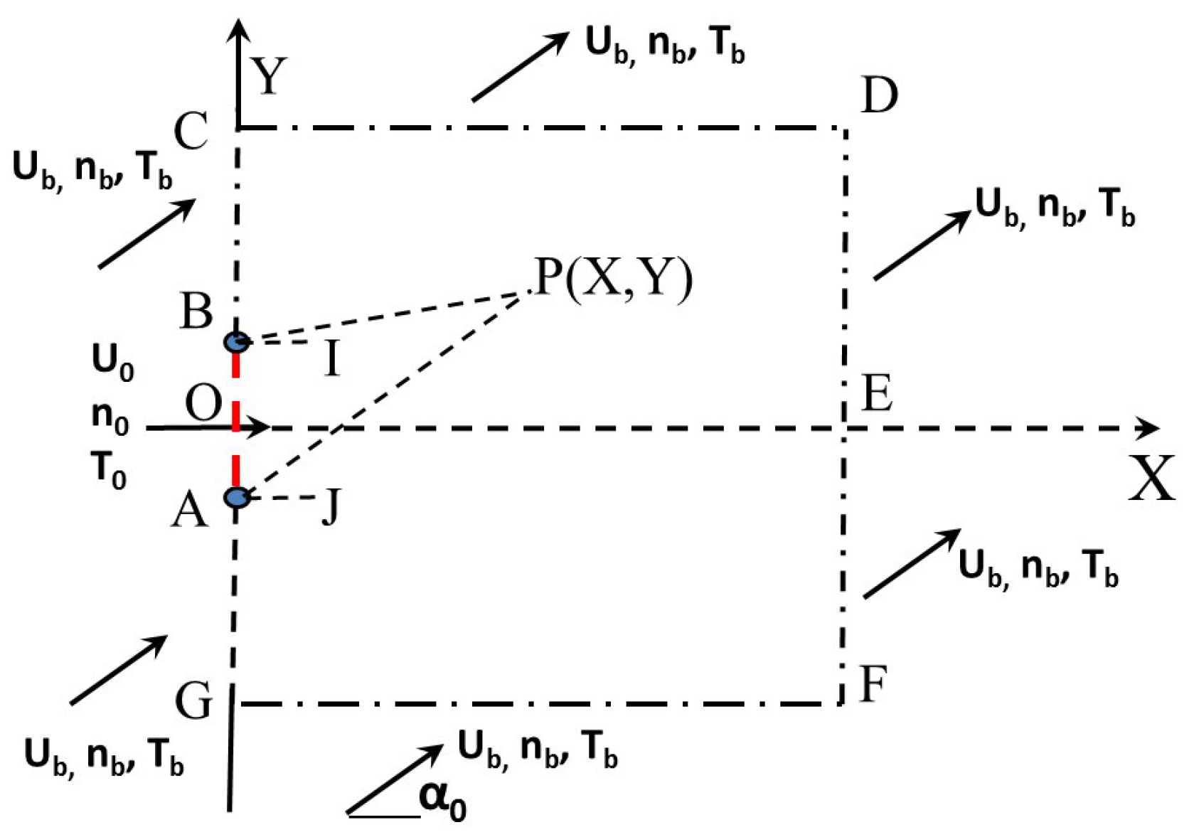
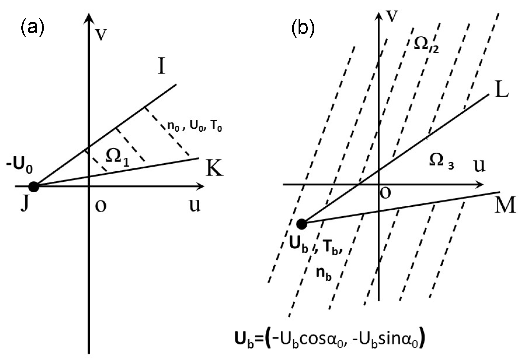
2. Collisionless Jet Expanding into a Uniform Dilute Background Flow

2.1. Derivations for the Mixture Density, Velocities, Temperature, and Pressure

Figure 1 illustrates the problem. In general, combined plume and background gas flows are three-dimensional. A simpler two-dimensional flow model is presented in this paper to demonstrate the procedure; however, it can conveniently extend to a three-dimensional situation. The problem can be summarized as follows. A collisionless jet expands into a near-vacuum place with a uniform dilute background flow. The jet and background flows are assumed to be described by Maxwellian velocity distribution functions, characterized by two bulk number densities $n_0$ and $n_b$, two bulk speeds $U_0$ and $U_b$, two temperatures $T_0$ and $T_b$, and the relative angle between these two flows defined as ${\alpha }_0$. The values for these seven parameters are assumed available. The nozzle exit is represented by segment $AoB$ in Figure 1. The background flow enters the simulation domain through $BC$, $CD$, $DEF$, $FG$, and $GA$; all the boundary edges except segment $AoB$. The goal of this section is to obtain formulas for the final mixture properties, including density, velocity components, pressure, and temperature.

The work in this paper is based on the classical gaskinetic theory [20], with the following definitions. At a specific flowfield point $P(X,Y)$, if there are several groups of molecules, their velocity distribution functions are $f_i$, and their corresponding velocity phase domains are ${\mathsf{\Omega }}_i$, then the bulk number density, velocity, and temperature at point $P(X,Y)$ can be computed as:

$$\begin{array}{ccc}\hfill n(X,Y)& =\hfill & {\displaystyle \sum _i}{\int }_{{\mathsf{\Omega }}_i}{f}_{i}dudvdw,\hfill \\ \hfill U(X,Y)& =\hfill & \frac{1}{n(X,Y)}{\displaystyle \sum _i}{\int }_{{\mathsf{\Omega }}_i}{u}_i{f}_{i}dudvw,\hfill \\ \hfill V(X,Y)& =\hfill & \frac{1}{n(X,Y)}{\displaystyle \sum _i}{\int }_{{\mathsf{\Omega }}_i}{v}_i{f}_{i}dudvdw,\hfill \\ \hfill T(X,Y)& =\hfill & \frac{1}{3Rn(X,Y)}{\displaystyle \sum _i}{\int }_{{\mathsf{\Omega }}_i}[{(u_i-U)}^2+{(v_i-V)}^2+w_i^2]f_{i}dudvdw\hfill \end{array}$$

(1)

where $u_i$, $v_i$, and $w_i$ are the instantaneous velocity components. The local pressure for point $P(X,Y)$ can be computed by using the equation of state.

The problem of a collisionless free jet expanding into a vacuum from an exit with different shapes was investigated in the past, and there are complete flowfield solutions for jet number density, velocity components, temperature, and pressure [23,24]. For a two-dimensional collisionless jet flow, the results are listed as follows:

$$\begin{array}{ccc}\hfill \frac{n_j(X,Y)}{n_0}& =\hfill & \frac{{\theta }_2-{\theta }_1}{2\pi }{e}^{-S_0^2}+\frac{1}{4}\left[\mathrm{erf}\left(S_0\sin {\theta }_2\right)-\mathrm{erf}\left(S_0\sin {\theta }_1\right)\right]+\frac{e^{-S_0^2}}{2\sqrt{\pi }}{\int }_{{\theta }_1}^{{\theta }_2}a{e}^{a^2}\mathrm{erf}\left(a\right)d\theta ,\hfill \end{array}$$

(2)

$$\begin{array}{ccc}\hfill \frac{n_j}{n_0}\frac{U_j(X,Y)}{\sqrt{2R{T}_0}}& =\hfill & \frac{e^{-S_0^2}}{4\pi }\{S_0({\theta }_2-{\theta }_1)+\frac{S_0}{2}\left[\sin \left(2{\theta }_2\right)-\sin \left(2{\theta }_1\right)\right]\hfill \\ & & +\sqrt{\pi }{\int }_{{\theta }_1}^{{\theta }_2}(1+2a^2)\cos \theta e^{a^2}\left[1+\mathrm{erf}\left(a\right)\right]d\theta \},\hfill \end{array}$$

(3)

$$\begin{array}{ccc}\hfill \frac{n_j}{n_0}\frac{V_j(X,Y)}{\sqrt{2R{T}_0}}& =\hfill & \frac{1}{4\sqrt{\pi }}\{\exp (-S_0^2{\sin }^2{\theta }_1)\cos {\theta }_1\left[1+\mathrm{erf}\left(S_0\cos {\theta }_1\right)\right]\hfill \\ & & -\exp (-S_0^2{\sin }^2{\theta }_2)\cos {\theta }_2\left[1+\mathrm{erf}\left(S_0\cos {\theta }_2\right)\right]\},\hfill \end{array}$$

(4)

$$\frac{T_j(X,Y)}{T_0}=-\frac{U_j^2+V_j^2}{3R{T}_0}+\frac{2e^{-S_0^2}}{3\pi }\frac{n_0}{n_j}{\int }_{{\theta }_1}^{{\theta }_2}{B}_0\left(a\right)d\theta ,$$

(5)

$$B_0\left(a\right)=\frac{\sqrt{\pi }}{4}[1+\mathrm{erf}\left(a\right)]e^{a^2}(4a+2a^3)+\frac{3}{4}+\frac{a^2}{2},$$

(6)

where “$j$” is for jet property, $S_0=U_0/\sqrt{2R{T}_0}$ is the specific speed ratio for the jet flow, $\theta =\mathrm{atan}(Y/X)$, ${\theta }_1=\mathrm{atan}\left((Y-H)/X\right)$, ${\theta }_2=\mathrm{atan}\left((Y+H)/X\right)$, H is the semi-height of the nozzle exit, and $a=S_0\cos \theta$. It shall be pointed out that, Noller [28] proposed a “starter surface” method to describe how to compute the jet density. The work in this paper is related but with significant differences. For example, the exact expression for jet density is accurately derived and presented in this paper, not in a descriptive manner. Only with this accurate formula for the density, the formulas for velocity and temperature can be further derived.

The problem of a jet expanding into a uniform, dilute background flow can be investigated with the gaskinetic theory as well, by following the same procedure as the simple jet situation [23]. An extra integration domain for the background gas flow is needed, and the combined domains ${\mathsf{\Omega }}_1$, ${\mathsf{\Omega }}_2$ for the combined flows are shown in Figure 2. Two groups of molecules from the jet and the background are assumed neutral and collisionless. Starting from Equation (1), with quite lengthy derivations, the following final combined flowfield results are obtained:

$$\begin{array}{ccc}\hfill \frac{n_m(X,Y)}{n_0}& =\hfill & -\frac{{\theta }_2-{\theta }_1}{2\pi }\frac{n_b}{n_0}{e}^{-S_b^2}-\frac{1}{4}\frac{n_b}{n_0}\left[\mathrm{erf}\left(S_b\sin ({\theta }_2-{\alpha }_0)\right)-\mathrm{erf}\left(S_b\sin ({\theta }_1-{\alpha }_0)\right)\right]\hfill \\ & & -\frac{e^{-S_b^2}}{2\sqrt{\pi }}\frac{n_b}{n_0}{\int }_{{\theta }_1-{\alpha }_0}^{{\theta }_2-{\alpha }_0}b{e}^{b^2}\mathrm{erf}\left(b\right)d\theta +\frac{n_j(X,Y)}{n_0}+\frac{n_b}{n_0},\hfill \end{array}$$

(7)

$$\begin{array}{ccc}\hfill \frac{n_m(X,Y)U_m(X,Y)}{n_0\sqrt{2R{T}_0}}& =\hfill & \frac{n_j(X,Y)U_j(X,Y)}{n_0\sqrt{2R{T}_0}}+\frac{n_b{U}_b}{n_0\sqrt{2R{T}_0}}-\hfill \\ & & \frac{n_b}{n_0}\frac{e^{-S_b^2}}{\pi }\sqrt{\frac{T_b}{T_0}}{\int }_{{\theta }_1-{\alpha }_0}^{{\theta }_2-{\alpha }_0}\cos (\theta +{\alpha }_0)\left[\frac{\sqrt{\pi }}{4}{e}^{b^2}\left[1+erf\left(b\right)\right](1+2b^2)+\frac{b}{2}\right]d\theta ,\hfill \end{array}$$

(8)

$$\begin{array}{ccc}\hfill \frac{n_m(X,Y)V_m(X,Y)}{n_0\sqrt{2R{T}_0}}& =\hfill & \frac{n_j(X,Y)V_j(X,Y)}{n_0\sqrt{2R{T}_0}}+\frac{n_b{V}_b}{n_0\sqrt{2R{T}_0}}-\hfill \\ & & \frac{n_b}{n_0}\frac{e^{-S_b^2}}{\pi }\sqrt{\frac{T_b}{T_0}}{\int }_{{\theta }_1-{\alpha }_0}^{{\theta }_2-{\alpha }_0}\sin (\theta +{\alpha }_0)\left[\frac{\sqrt{\pi }}{4}{e}^{b^2}\left[1+\mathrm{erf}\left(b\right)\right](1+2b^2)+\frac{b}{2}\right]d\theta ,\hfill \end{array}$$

(9)

$$\frac{T_m(X,Y)}{T_0}=-\frac{U_m^2+V_m^2}{3R{T}_0}+\frac{2}{3}\frac{n_0}{n_m}\left(\frac{e^{-S_0^2}}{\pi }{\int }_{{\theta }_1}^{{\theta }_2}{B}_0\left(a\right)d\theta +\frac{e^{-S_b^2}}{\pi }\frac{n_b}{n_0}\frac{T_b}{T_0}{\int }_{{\theta }_2-{\alpha }_0}^{{\theta }_1+2\pi -{\alpha }_0}{B}_0\left(b\right)d\theta \right),$$

(10)

$$\frac{p_m(X,Y)}{p_0}=\frac{n_m{T}_m}{n_0{T}_0},$$

(11)

where subscript “m” represents a mixture property; subscript “b” represents a background flow property; $S_b=\sqrt{(U_b^2+V_b^2)/\left(2R{T}_b\right)}$; $U_b=S_b\sqrt{2R{T}_b}\cos {\alpha }_0$; $V_b=S_b\sqrt{2R{T}_b}\sin {\alpha }_0$; and $b=S_b\cos \theta$. Formulas for $n_j$, $U_j$, and $V_j$ are Equations (2)–(4). Flowfield temperature and pressure for the jet/background gas mixture are obtained, by following flowfield properties of non-dimensional number density and velocity components.

If the angle between the X-axis and line $OP$ in Figure 1 is defined as $\lambda \equiv \mathrm{atan}(Y/X)$, then from Equations (8) and (9), the normalized mixture number flux along the radial direction can be computed:

$$\begin{array}{ccc}\hfill \frac{{\dot{n}}_m}{n_0\sqrt{2R{T}_0}}& =\hfill & \frac{n_m(U_m\cos \lambda +V_m\sin \lambda )}{n_0\sqrt{2R{T}_0}}=\frac{n_j(U_j\cos \lambda +V_j\sin \lambda )+n_b(U_b\cos \lambda +V_b\sin \lambda )}{n_0\sqrt{2R{T}_0}}-\hfill \\ & & \frac{n_b}{n_0}\frac{e^{-S_b^2}}{\pi }\sqrt{\frac{T_b}{T_0}}{\int }_{{\theta }_1-{\alpha }_0}^{{\theta }_2-{\alpha }_0}\cos (\theta +{\alpha }_0-\lambda )\left[\frac{\sqrt{\pi }}{4}{e}^{b^2}\left[1+\mathrm{erf}\left(b\right)\right](1+2b^2)+\frac{b}{2}\right]d\theta .\hfill \end{array}$$

(12)

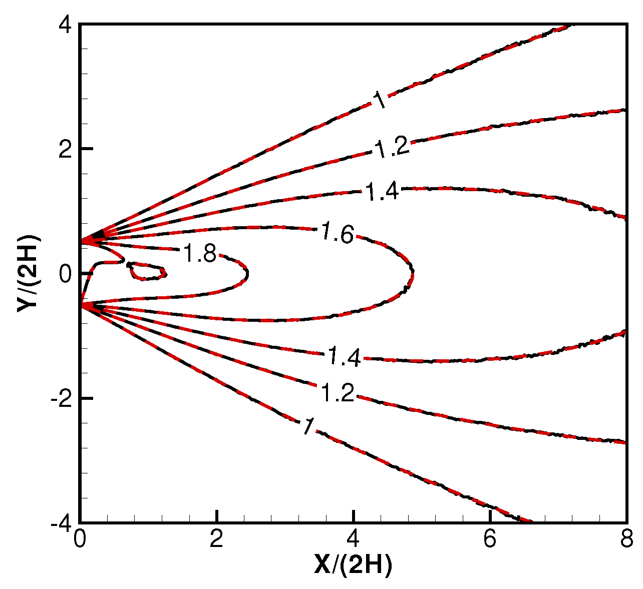
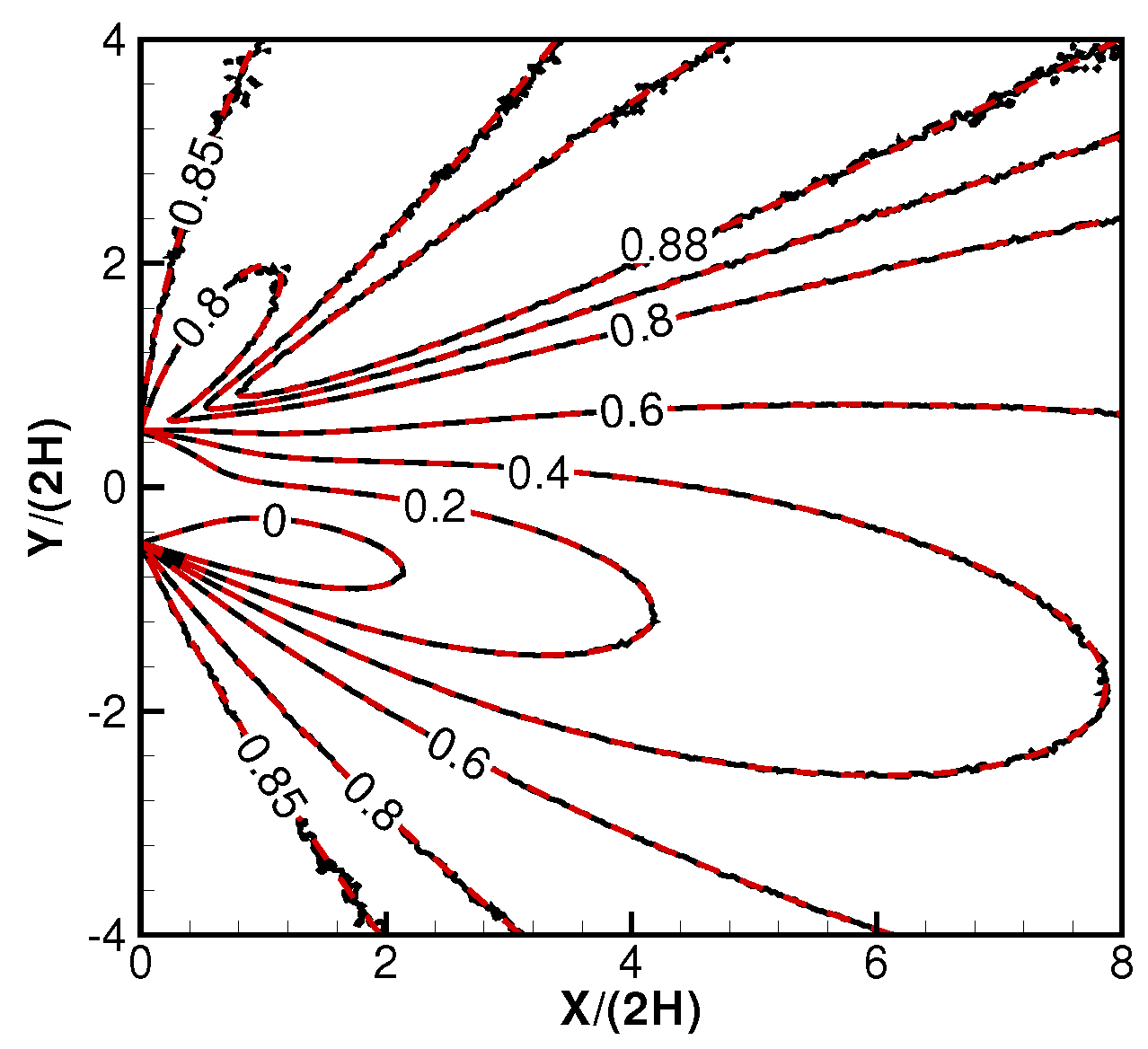
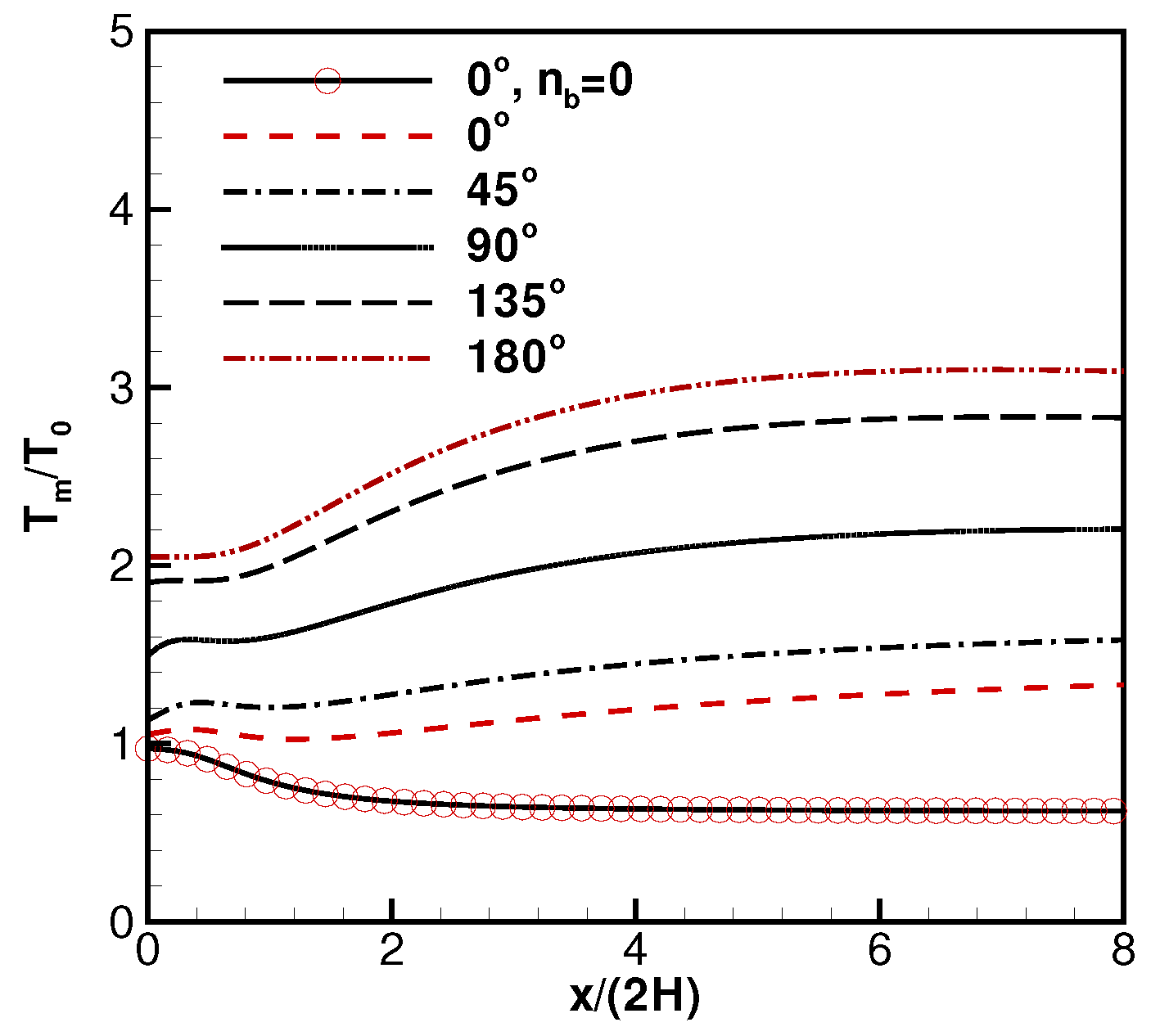
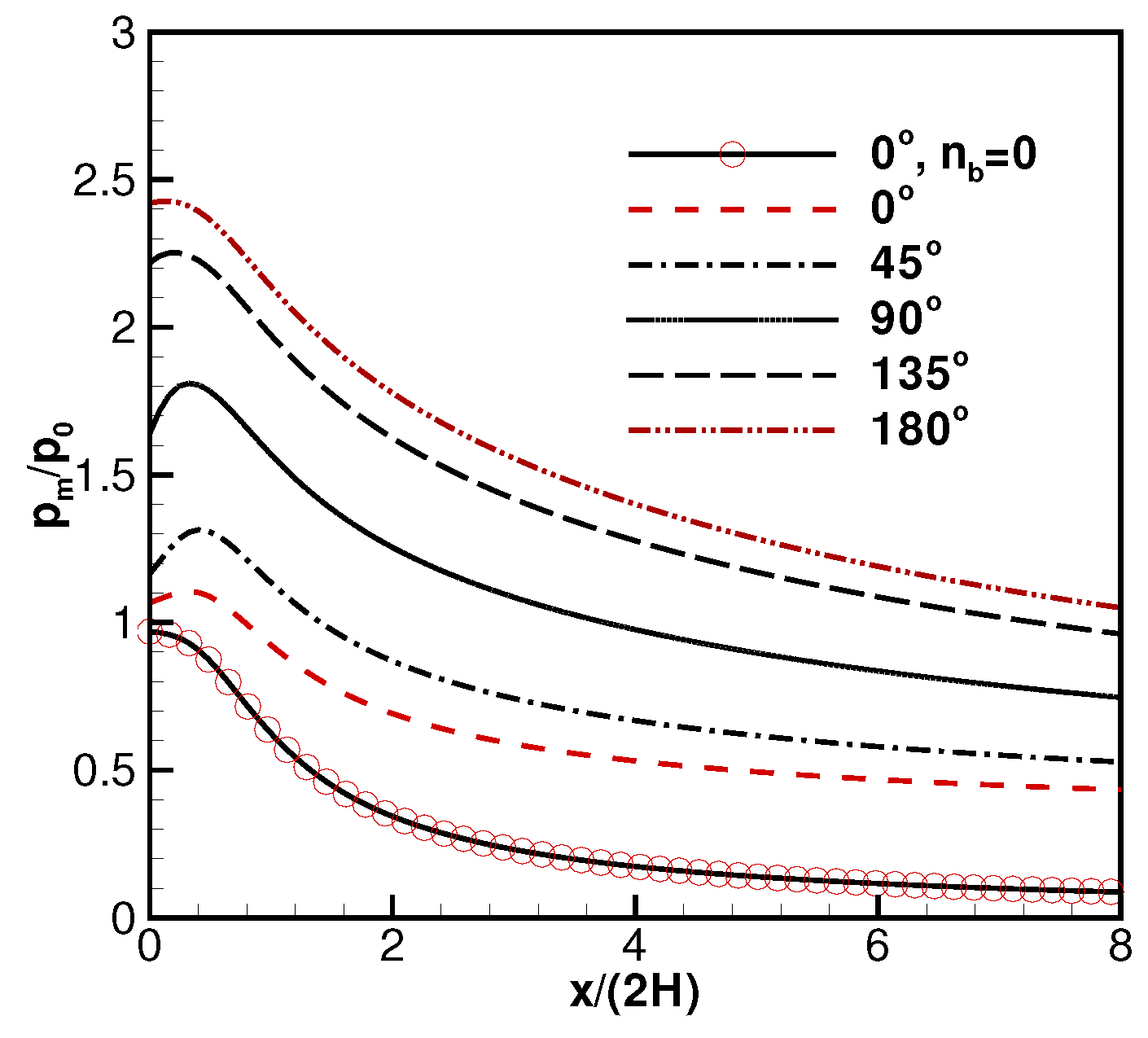
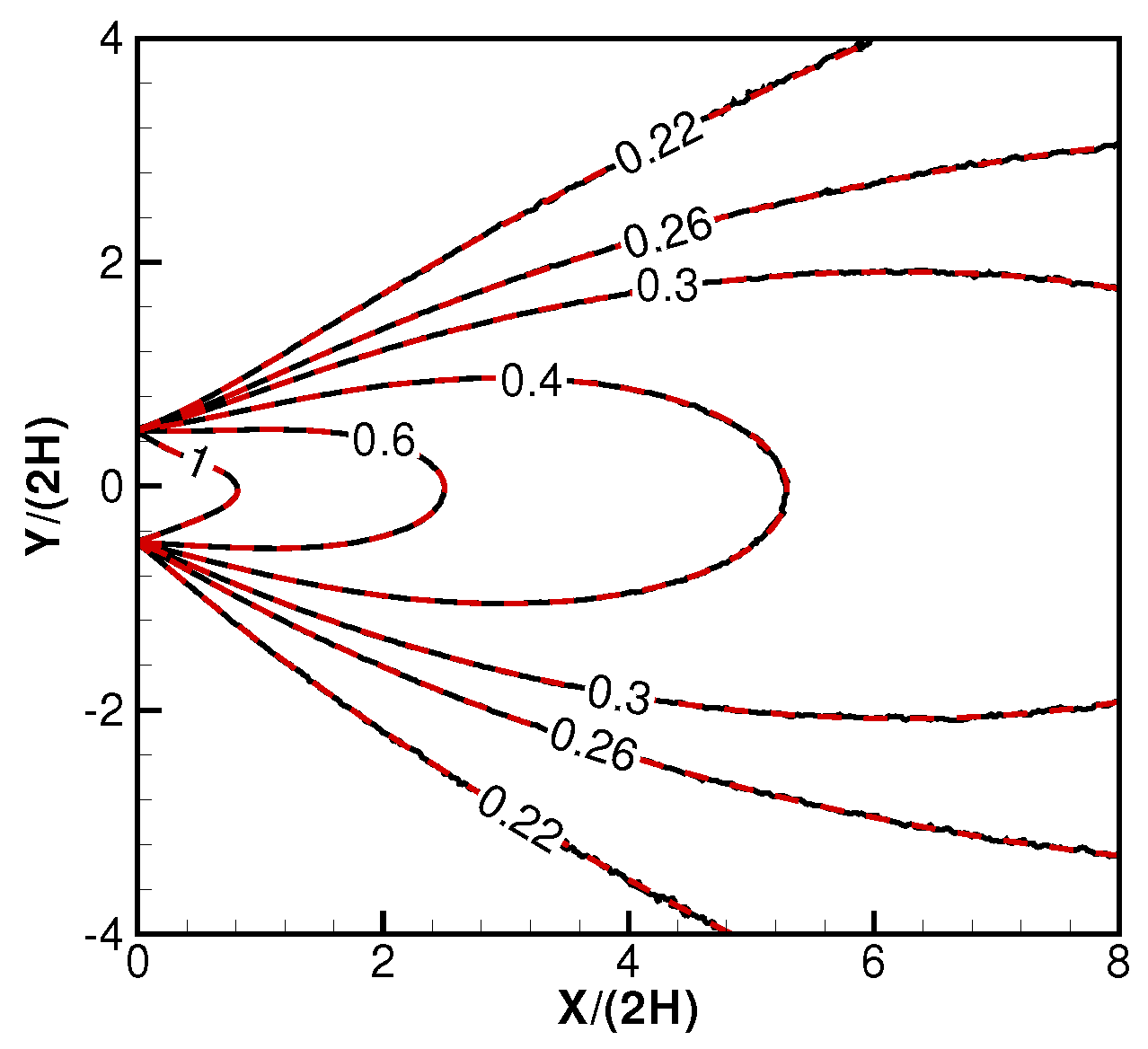
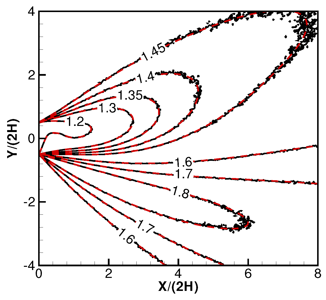
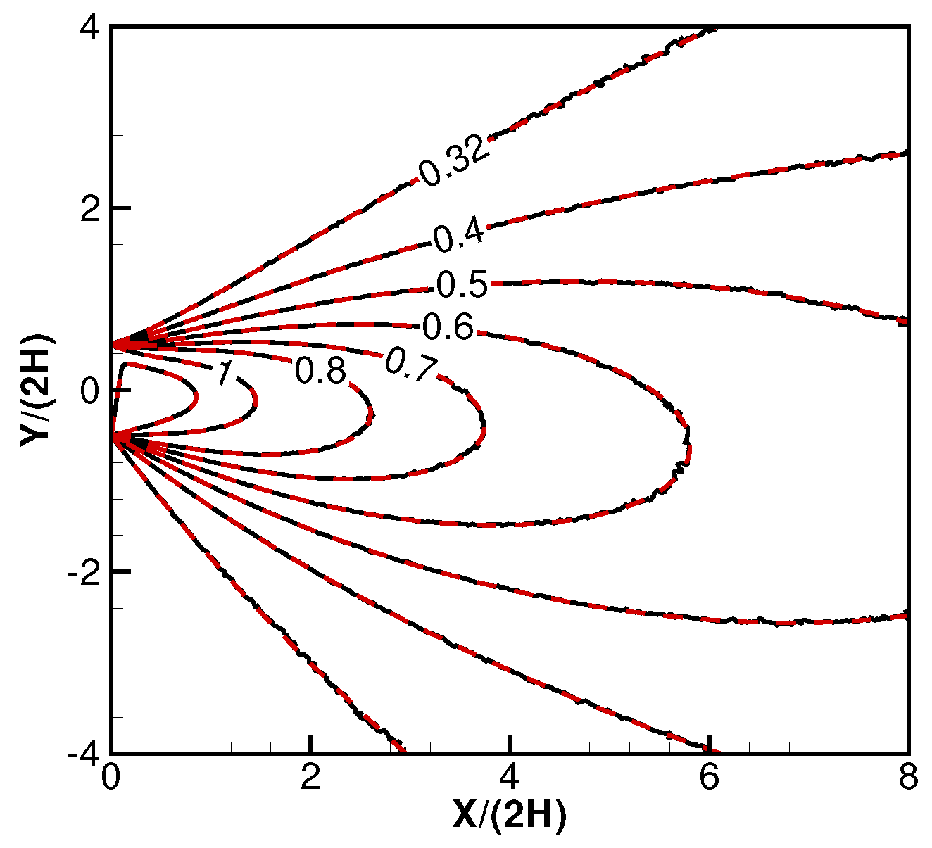
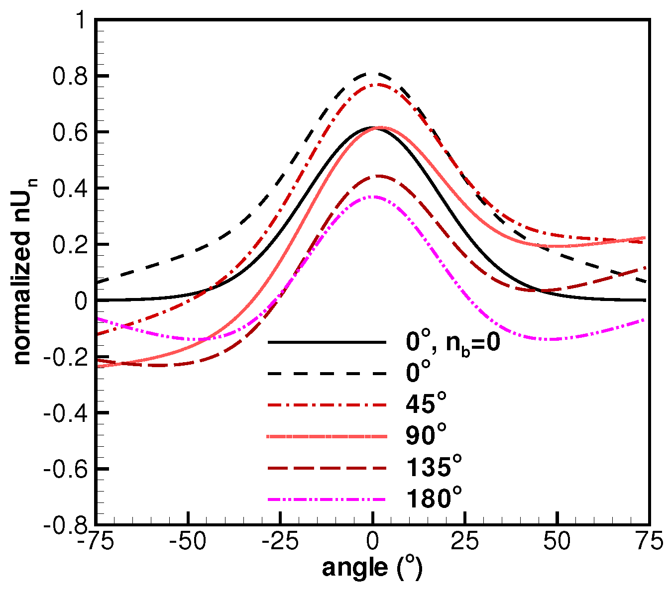
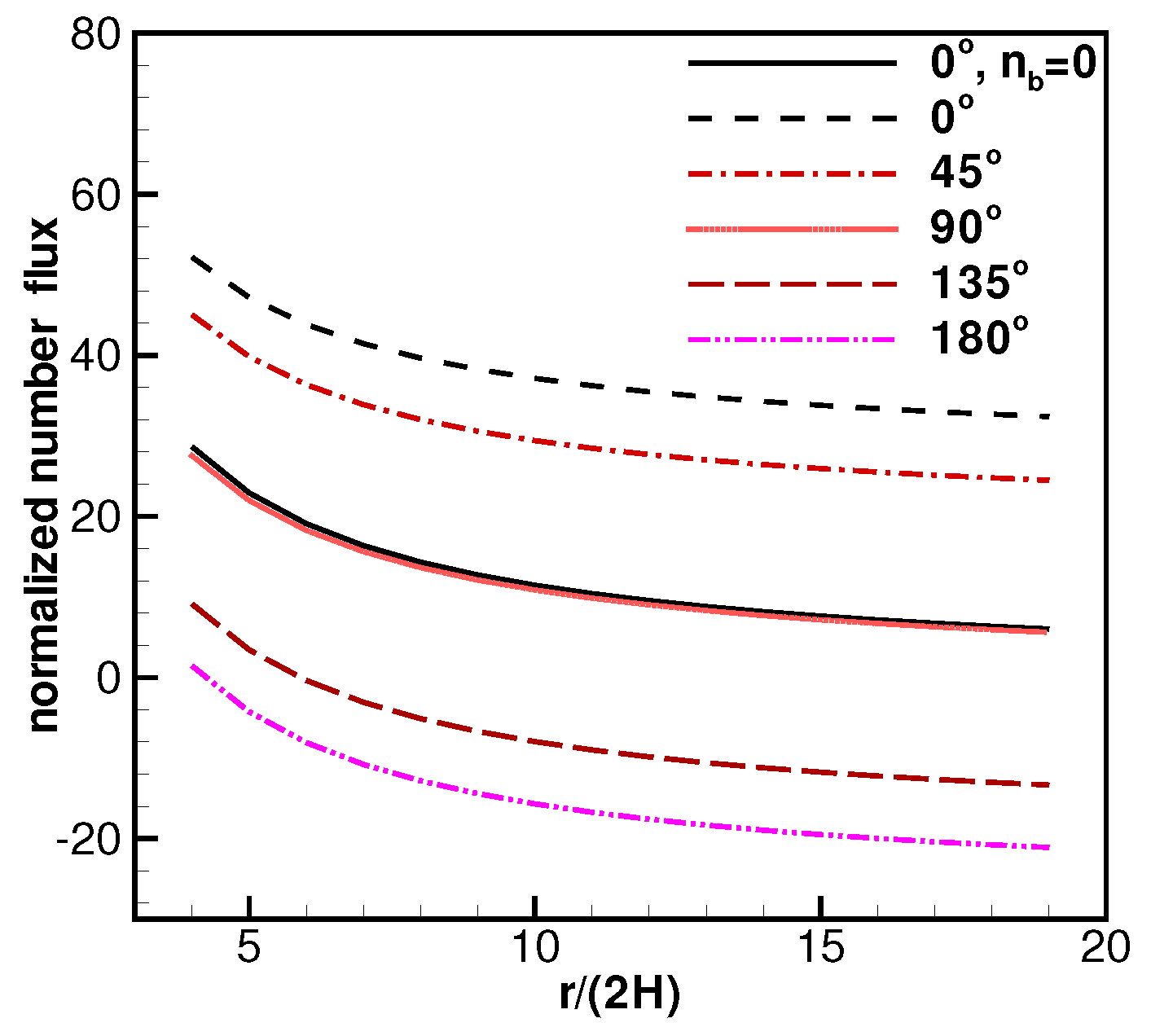
2.2. Validations and Discussions on the Derived Formulas

Equations (7)–(11) are complex with several non-dimensional parameters; hence, numerical evaluations and validations are necessary. A specific DSMC simulation package named GRASP [29] is adopted for the simulations. Argon gas is assumed as the rarefied jet and background flows. Figure 1 shows the boundary conditions. Line $AoB$ is treated as a jet exit and an inlet into the simulation domain. The rest of the simulation domain boundaries are treated as inlets for the collisionless background flow. For DSMC simulations, an inlet boundary condition means within each time step, a certain number of simulation particles are introduced into the simulation domain from that boundary, and a particle is removed from the simulation if it hits that boundary from inside. It shall be emphasized that the background particles are introduced into the domain from all the boundaries except segment $AoB$—the nozzle exit blocks the background flow particles. The flow is collisionless with an infinitely large Knudsen number, and the DSMC simulations assume no collisions.

A DSMC simulation is performed to validate the whole flow field solutions with the following simulation parameters: $n_b/n_0=0.2$, $S_0=2$, ${\alpha }_0={45}^{\circ }$, $S_b=1.0$, $T_0=200$ Kelvin, and $T_b=300$ Kelvin. The jet number density $n_0$ is chosen to be $1\times {10}^{10}$ m${}^{-3}$. These numbers are randomly selected to demonstrate the overall effects. The height and width for the whole simulation domain are set as 8 m, i.e., segments $DEF$, $GF$, $GABC$, and $CD$ in Figure 1, and the nozzle exit width $AB$ is 1 m.

Figure 3 shows the normalized density contours, $n_m/n_0$. The gradients around the exit are fairly large, and the two nozzle exit lips are singularity points where the density drops rapidly to the background density outside the nozzle. Figure 4 and Figure 5 show contours for normalized mixture velocity components, $U_m/\sqrt{2R{T}_0}$ and $V_m/\sqrt{2R{T}_0}$, along the X- and Y-directions, respectively. Due to the background flows, the velocity contours, especially for the V-velocity component, are distorted. For the U-velocity component contours, the topology patterns change from the scenario of a collisionless jet expanding into a true vacuum, where the velocity continues to increase monotonically along the X-direction [23]. Figure 6 and Figure 7 are normalized temperature and pressure contours, $T_m/T_0$ and $p_m/p_0$. The analytical and numerical simulation results are essentially identical, and the simulation results validate Equations (7)–(11), for the combined flowfield with jet and background flows. These validated formulas provide solid foundations for further discussions, and no extra simulations are needed.

Figure 8, Figure 9, Figure 10 and Figure 11 present several jet centerline properties, calculated with Equations (7), (8), (10) and (11). The parameters are: $n_b/n_0=0.2$, $S_0=2$, $S_b=1$, $T_0=200$ Kelvin, and $T_b=300$ Kelvin, and the background flow direction ${\alpha }_0$ varies to demonstrate the background flow effects on the primary jet flows. Figure 8 shows the centerline density profiles. Circular symbols are added on the pure jet curve for clarity. For mixed flows, the scenarios of ${\alpha }_0=0^{\circ }$ and ${180}^{\circ }$ form two bounding limits, and all the curves for mixed flows have an asymptote of $n_b/n_0=0.2$ at farfield. By comparison, the profile for a pure jet scenario approaches zero at farfield. This figure demonstrates that the effects from the background density shall be quantified. For example, in the upper atmosphere, the background density decreases at higher altitudes and the effects may diminish.

Figure 9 shows the non-dimensional centerline U-velocity profiles for the mixture. The curve for the pure jet scenario (i.e., $n_b=0$) continues to accelerate along the centerline because fast molecules have larger opportunities to be observed at downstream. For other situations with background flows ($n_b>0$), eventually the centerline velocity profiles merge into the slow background flows. This figure warns us that a measured velocity in a vacuum chamber may not represent the free jet flows at farfield. The background flow with ${\alpha }_0=0^{\circ }$ has the highest mixed velocity while the ${\alpha }_0={180}^{\circ }$ case has the lowest averaged centerline velocity. Low speed background flows, such as inside a ground vacuum chamber, completely change the jet centerline speeds from accelerations to deceleration. The speed for the background flow at upper atmosphere orbit is about $7.9$ km/s that the jet flow shall merge into; hence, it is understandable that the flowfield patterns inside a ground vacuum chamber and at a high altitude are different.

Figure 10 shows the non-dimensional centerline temperature profiles for the jet/background flow mixture. The relatively hotter background flow changes the farfield profiles. For the pure free jet situation with $n_b=0$, at farfield, faster molecules have larger opportunities to appear and their velocity deviations from their local bulk velocities become smaller, resulting in a decreasing temperature profile. However, for mixed flows with $n_b>0$, they must eventually merge into the hot background flow ($T_0=200$ Kelvin $<T_b=300$ Kelvin). In a ground vacuum chamber, a room temperature is proper to describe the background flows, but at upper atmosphere, the temperature is low. This figure indicates that the background flow temperature effects shall be carefully quantified.

Figure 11 shows the non-dimensional centerline pressure profiles for the mixture, where the pure jet flow case ($n_b=0$) has the lowest value. With background flows, different ${\alpha }_0$ values affect the final mixture pressure. For example, ${\alpha }_0=0^{\circ }$ leads to a low pressure. Figure 12 shows the number flux for the mixture, along a constant radius, $r/\left(2H\right)=4$, and the angle span formed by the curve ends and the exit center is $-{75}^{\circ }<\theta <{75}^{\circ }$. All the other parameters remain the same as the above test case for the centerline profiles. For the pure jet situation without background flows, the number flux profile is symmetric. For the other test cases with background flows $n_b>0$ but different ${\alpha }_0$ values, most number flux profiles are distorted and asymmetric. For the situations with ${\alpha }_0=0^{\circ }$ or ${180}^{\circ }$, the profiles are symmetric about the centerline. Figure 11 and Figure 12 can explain Yim and Burt’s conclusion [19] that different pump locations may affect the measured experimental data. Because vacuum pumps remove gas molecules and form local background flows towards the pumps, different pump locations create different local ${\alpha }_0$ values. As can be understood, different vacuum chambers installed different types of pumps at different locations. These two figures show adverse facility or background flow effects due to different flow directions.

Usually, for jet flows inside vacuum chambers, a collisionless flow is a reasonable assumption due to the related low jet and background flow densities. At the farfield boundaries, the nozzle exit can be considered as a point source. It is generally accepted that there is a constant total number flux across an arc within the same angle span but of different radius. As shown in Figure 13, for the pure jet situation with $n_b=0$, the integration results of mass flux over curves $AB$ and $DC$ shall be the same. This assumption is not always valid with a background flow. If there is a uniform background flow, e.g., assuming from left to right with ${\alpha }_0=0^{\circ }$, the background number flux through $CD$ shall be larger than that through $AB$, because the former curve has a larger width. The total number fluxes through $CD$ and $AB$ shall be larger than that out of the nozzle exit. By comparison, if the background flow is from right to left with ${\alpha }_0={180}^{\circ }$, then a portion of jet flux is “canceled” by the background flows. The measured total number flux across curve $CD$ shall be smaller than that across $AB$, and both are smaller than that out of the nozzle. Figure 14 shows the integrated total number flux with different radii, within an angle span of $-{75}^{\circ }<\theta <{75}^{\circ }$. For the scenario of a pure jet into a true vacuum, $n_b=0$, the total number flux conservation relation holds. For the situation that the background flow is not perpendicular to the jet flow, the number flux curve is shifted from the pure jet flow case.

In summary, Figure 3, Figure 4, Figure 5, Figure 6 and Figure 7 confirm that with the seven known parameters characterizing the jet and background flows, the new formulas accurately predict the background flow effects. The background facility effects may be undesirable, and further investigations are necessary. Plume property patterns can completely change with opposite trends, even within a short distance from the exit.

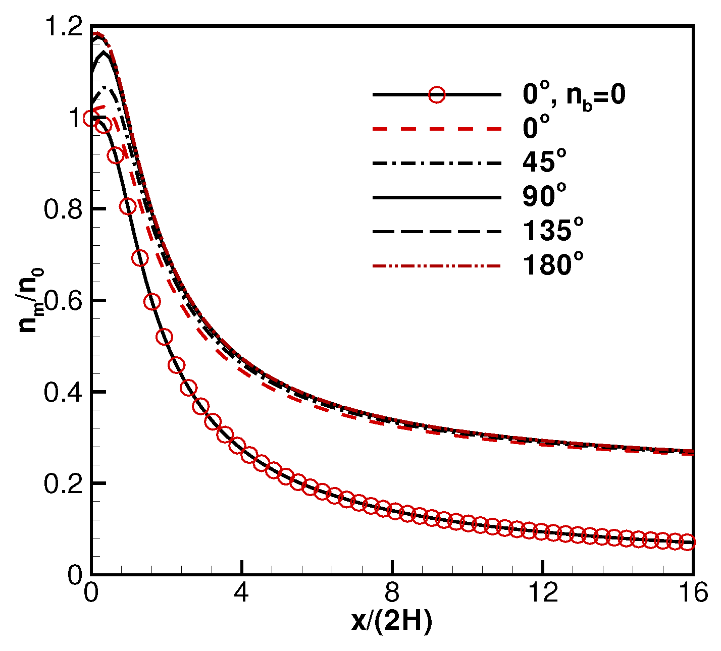
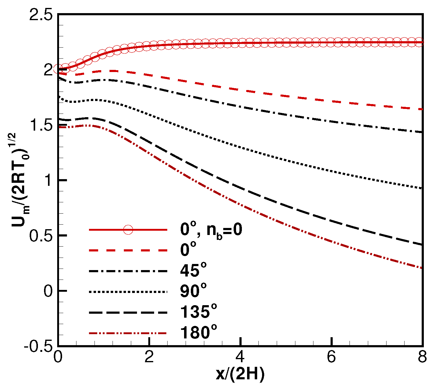
2.3. Background Flow Effects on Electric Propulsion (EP) Devices’ Performance

If the background flow parameters are available, then the background flow impacts on an EP device can be estimated conveniently with the gaskinetic theory. For example, a certain amount of background gas may enter the EP devices, and the mass flow ratio can be computed as:

$$\begin{array}{ccc}\hfill \frac{{\dot{m}}_b}{{\dot{m}}_j}& =\hfill & -n_b\sqrt{\frac{{\beta }_b}{\pi }}{\int }_{-\infty }^{0}u{e}^{-{(u-S_b\sqrt{2R{T}_b}\cos {\alpha }_0)}^2/\left(2R{T}_b\right)}du/(n_0\sqrt{\frac{{\beta }_0}{\pi }}{\int }_0^{\infty }u{e}^{-{(u-U_0)}^2/\left(2R{T}_0\right)}du)\hfill \\ & =\hfill & \frac{n_b}{n_0}\sqrt{\frac{T_0}{T_b}}\frac{S_b\cos {\alpha }_0\sqrt{\pi }[1+\mathrm{erf}\left(S_b\cos {\alpha }_0\right)]-2S_b\cos {\alpha }_0+e^{-S_b^2{\cos }^2{\alpha }_0}}{S_0\sqrt{\pi }[1+\mathrm{erf}\left(S_0\right)]+e^{-S_0^2}}\hfill \end{array}$$

(13)

where ${\dot{m}}_b$ is the amount of background gas entering the exit, and ${\dot{m}}_j$ is the jet flow out of the exit.

The extra forces on the EP devices due to the background flow consist of at least three terms: (1) the pressure force components on the device surface along the jet direction; (2) the shear stress force components on the device surface along the jet direction; and (3) the force to reverse the background flow direction, or at least to stop background gas flow into the devices. It shall be emphasized that there may be lateral forces and moments on the device as well. Many factors may affect the results, such as, the EP device geometries, and the relative flow angle ${\alpha }_0$ between the jet and background flows, the temperature ratio, and the speed ratios.

It can be shown that the force to stop the background flow gas into the device is:

$$\frac{F_0}{\left(2R{T}_b\right)n_{b}m{A}_{exit}}=\left(\frac{1}{4}+\frac{1}{2}{S}_b^2{\cos }^2{\alpha }_0\right)[1-\mathrm{erf}\left(S_b\cos {\alpha }_0\right)]-\frac{S_b\cos {\alpha }_0}{2\sqrt{\pi }}{e}^{-S_b^2{\cos }^2{\alpha }_0}$$

(14)

where $A_{exit}$ is the nozzle exit area.

The pressure forces acting on the back and front sides of the device can also be computed. For simplicity, these two surfaces are assumed flat. Then the force on a specular reflective surface is:

$$\frac{F_1}{\left(2R{T}_b\right)n_{b}m{A}_b}=\left(\frac{1}{2}+S_b^2{\cos }^2{\alpha }_0\right)[1+\mathrm{erf}\left(S_b\cos {\alpha }_0\right)]+\frac{S_b\cos {\alpha }_0}{\sqrt{\pi }}{e}^{-S_b^2{\cos }^2{\alpha }_0}$$

(15)

where $A_b$ is the area at the backside of the EP devices without the nozzle exit. The force acting on the other side of the device is:

$$\frac{F_2}{\left(2R{T}_b\right)n_{b}m{A}_f}=\left(\frac{1}{2}+S_b^2{\cos }^2{\alpha }_0\right)[1-\mathrm{erf}\left(S_b\cos {\alpha }_0\right)]-\frac{S_b\cos {\alpha }_0}{\sqrt{\pi }}{e}^{-S_b^2{\cos }^2{\alpha }_0}$$

(16)

where $A_f$ is the solid surface area at the other side with the nozzle exit.

It is also possible to compute the pressure forces on a diffuse surface, which are related with the mass flow rates for background gas flows impinging on the back and front surfaces:

$$\frac{{\dot{m}}_1}{n_{b}m{A}_b}=\sqrt{\frac{{\beta }_b}{\pi }}{\int }_0^{+\infty }u{e}^{-{\beta }_b{(u-U_b)}^2}du=\frac{S_b\cos {\alpha }_0}{2}\sqrt{2R{T}_b}[1+\mathrm{erf}\left(S_b\cos {\alpha }_0\right)]+\sqrt{\frac{R{T}_b}{2\pi }}{e}^{-S_b^2{\cos }^2{\alpha }_0}$$

(17)

$$\frac{{\dot{m}}_2}{n_{b}m{A}_f}=\sqrt{\frac{{\beta }_b}{\pi }}{\int }_{-\infty }^{0}u{e}^{-{\beta }_b{(u-U_b)}^2}du=\frac{S_b\cos {\alpha }_0}{2}\sqrt{2R{T}_b}[1-\mathrm{erf}\left(S_b\cos {\alpha }_0\right)]-\sqrt{\frac{R{T}_b}{2\pi }}{e}^{-S_b^2{\cos }^2{\alpha }_0}$$

(18)

The corresponding pressure forces are:

$$F_3=\frac{F_1}{2}+\sqrt{\frac{\pi R{T}_w}{2}}{\dot{m}}_1;F_4=\frac{F_2}{2}+\sqrt{\frac{\pi R{T}_w}{2}}{\dot{m}}_2$$

(19)

The friction forces. lateral force, and moment on the device’s surface are closely related to its geometry, and they are all computable.

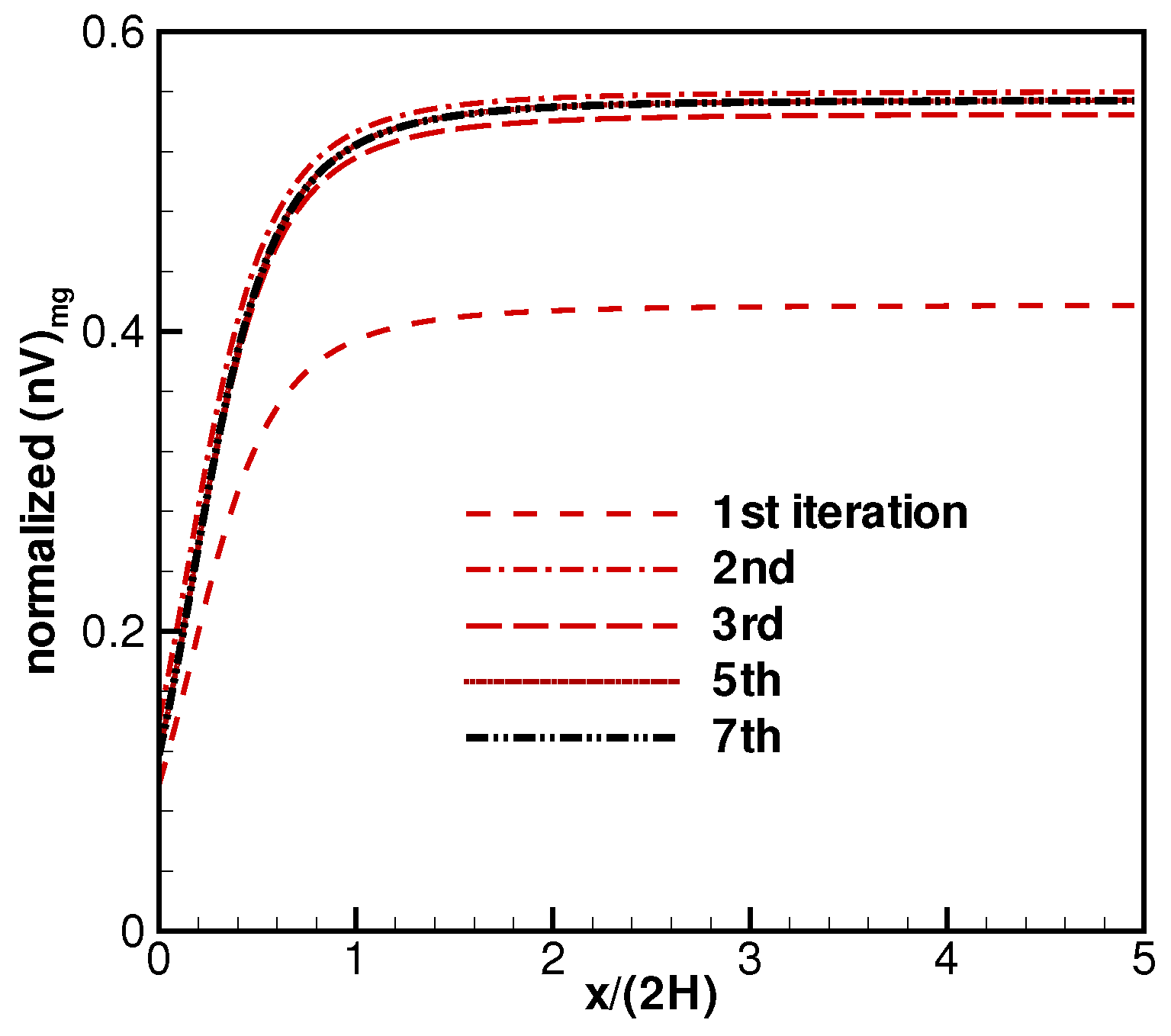
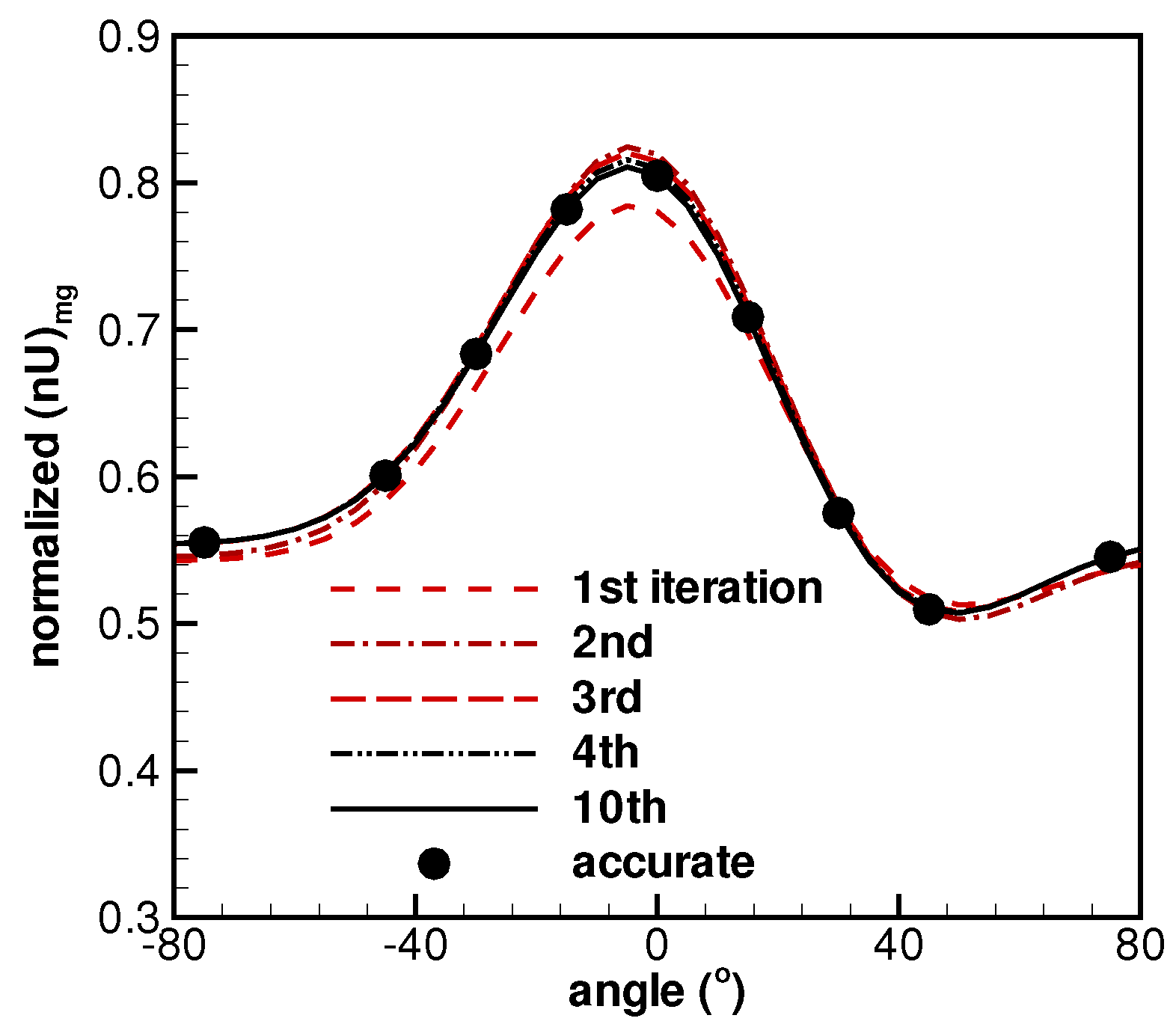
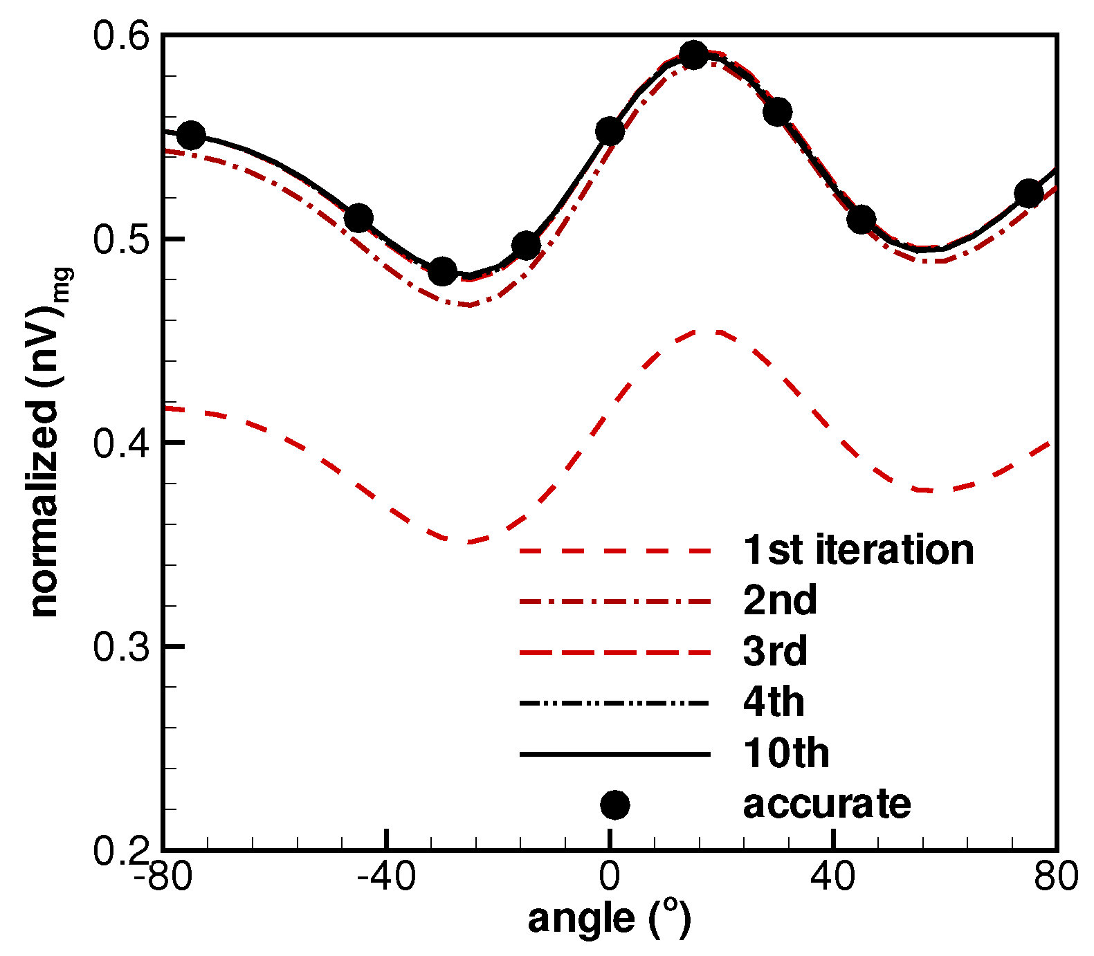
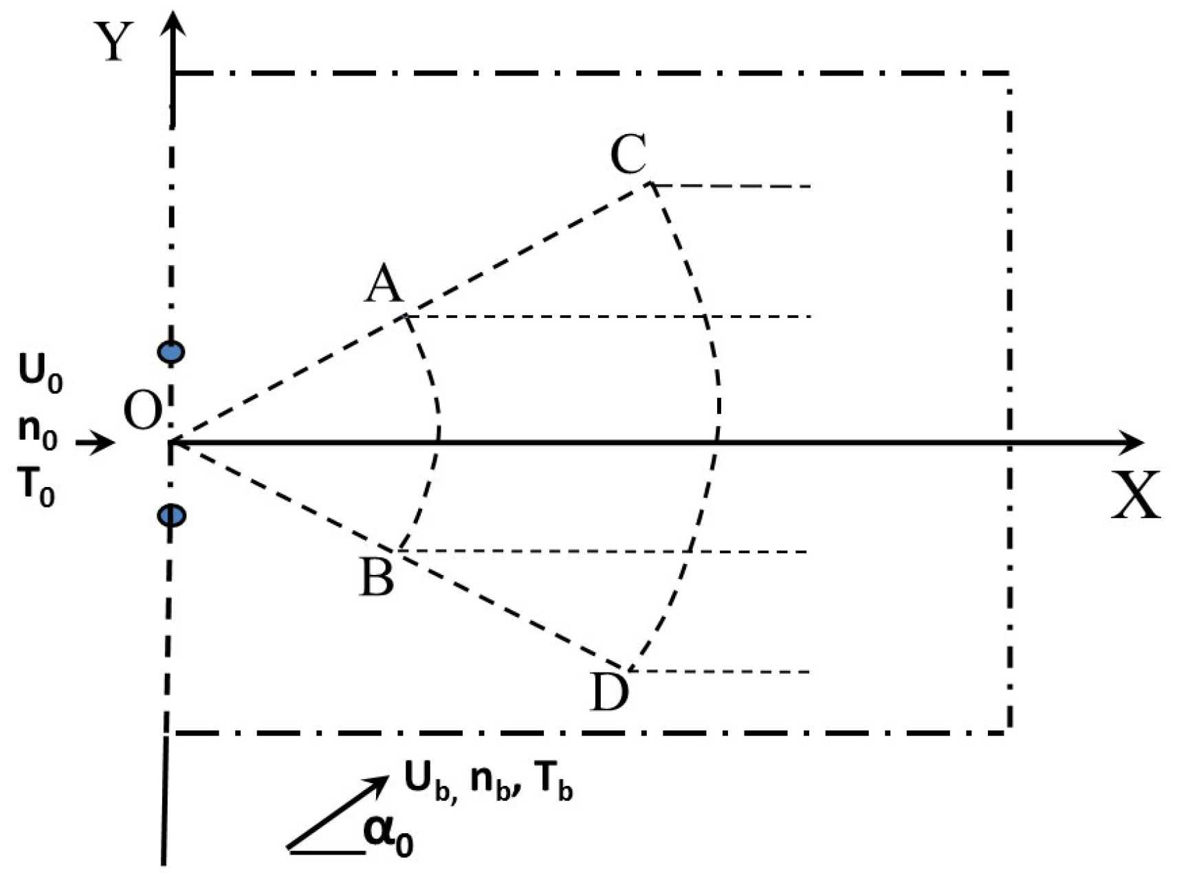
3. New Methods to Recover the Flow Parameters with Limited Measurements

The above section demonstrates how to determine the combined flowfield properties from background and jet flows, which are described by the seven parameters, $n_0$, $S_0$, $T_0$, $n_b$, $S_b$, $T_b$, and ${\alpha }_0$. The reverse problem is more practical and important: from limited experimental measurements, is it possible to recover the seven parameters? If DSMC simulations are adopted for this parameter recover work, then a large number of different parameter combinations must be assumed, and the simulations shall be performed in trial-and-error, just like shooting in dark, to find the combinations with the best match between the simulated results and the measurements. The procedure must be very lengthy because there is no information about towards which direction shall the parameters be tuned. This section aims to address this question with a new approach.

3.1. Linearized Governing Equations for the Density and Number Fluxes

Because there are seven parameters describing the rarefied background and jet flows, only seven relations or equations are needed, with a minimum of seven experimental measurements.

The critical step in this new method is to linearize Equations (7)–(9), for the number density and number fluxes. The process starts with good initial estimations on the seven parameters, denoted as $n_{0g}$, $S_{0g}$, $n_{bg}$, $S_{bg}$, ${\alpha }_{0g}$, $T_{0g}$ and $T_{bg}$, where the subscript $“g^{″}$ represents a guessed or estimated value. These guessed values are assumed to have small deviations from the corresponding true values, and a set of small perturbation parameters, ${ϵ}_i$, are introduced:

$$\begin{array}{ccc}\hfill n_0& =\hfill & n_{0g}(1+{ϵ}_1),S_0=S_{0g}(1+{ϵ}_2),n_b=n_{bg}(1+{ϵ}_3),S_b=S_{bg}(1+{ϵ}_4),\hfill \\ \hfill {\alpha }_0& =\hfill & {\alpha }_{0g}(1+{ϵ}_5),T_0=T_{0g}(1+{ϵ}_6),T_b=T_{bg}(1+{ϵ}_7).\hfill \end{array}$$

(20)

These seven guessed values will update by multiplying $1+{ϵ}_i$ after each iteration; hence, if these parameters ${ϵ}_i$ continue to decrease, then the guessed values approach to the true parameter values.

Equations (7)–(9) and (20) lead to the following linearized expressions:

$$A_1{ϵ}_1+A_2{ϵ}_2+A_3{ϵ}_3+A_4{ϵ}_4+A_5{ϵ}_5+{\left(n_m\right)}_g=n_m(X,Y),$$

(21)

$$B_1{ϵ}_1+B_2{ϵ}_2+B_3{ϵ}_3+B_4{ϵ}_4+B_5{ϵ}_5+B_6{ϵ}_6+B_7{ϵ}_7+{\left(n_m{U}_m\right)}_g=\left(n_m{U}_m\right)(X,Y),$$

(22)

$$C_1{ϵ}_1+C_2{ϵ}_2+C_3{ϵ}_3+C_4{ϵ}_4+C_5{ϵ}_5+C_6{ϵ}_6+C_7{ϵ}_7+{\left(n_m{V}_m\right)}_g=\left(n_m{V}_m\right)(X,Y),$$

(23)

where $A_i$, $B_i$ and $C_i$ are expressions with current estimated properties, and their specific expressions are included in the Appendix; the right hand side terms $n_m(X,Y)$, $\left(n_m{U}_m\right)(X,Y)$ and $\left(n_m{V}_m\right)(X,Y)$ represent measured number density, number fluxes along the X- and Y-directions; ${\left(n_m\right)}_g(X,Y)$, ${\left(n_m{U}_m\right)}_g(X,Y)$ and ${\left(n_m{V}_m\right)}_g(X,Y)$ represent the corresponding density and number flux values computed by using Equations (7)–(9) with the seven estimated parameters.

The expression for the mixture temperature is based on those expressions for the mixture number density and number fluxes, it is unnecessary to introduce a new perturbation parameter which shall be a combination of the other seven small perturbation parameters. It is inconvenient to use the temperature result for perturbations because the expressions are rather complex.

To determine the seven parameters can be achieved with different approaches. For example, by measuring the number densities, and number fluxes along the X- and Y- directions, at several points. The coefficients $A_i$, $B_i$, and $C_i$ have different values at each point, due to the different geometry factors, i.e., ${\theta }_1$ and ${\theta }_2$, and the local flowfield properties.

The new methods take the following steps to recover the seven parameters.

Step 1:

perform initial estimations on the seven parameters: $n_{0g}$, $S_{0g}$, $n_{bg}$, $S_{bg}$, ${\alpha }_{0g}$, $T_{0g}$ and $T_{bg}$;

Step 2:

select a total of $N_1$ measured densities $n_m$ at different points, $0\le N_1<6$;

Step 3:

select a total of $N_2$ measured number fluxes along the X-direction, ${\left(nU\right)}_m$, $N_2\ge 0$;

Step 4:

select a total of $N_3$ measured number fluxes along the Y-direction, ${\left(nV\right)}_m$, $N_3\ge 0$;

Here $N_1+N_2+N_3\ge 7$. The properties can be from the same or different points, e.g., measured number density and fluxes at one point offer three relations.

Step 5:

for each selected point, compute the corresponding ${\theta }_2$ and ${\theta }_1$;

Step 6:

for each of the $N_1$ measured densities, use ${\theta }_1$ and ${\theta }_2$, and the five guessed parameters, $n_{0g}$, $S_{0g}$, $n_{bg}$, $S_{bg}$, and ${\alpha }_{0g}$, to compute the corresponding $A_1$–$A_5$, and a total of $N_1$ guessed jet number number density $n_{jg}$ can be computed by using Equation (2). With the measured densities, $n_m$, a total of $N_1$ linear algebraic equations about ${ϵ}_1$–${ϵ}_5$, are properly constructed;

Step 7:

for each of the $N_2$ measured number fluxes along the X-direction, ${\left(nU\right)}_m$, by using the ${\theta }_1$ and ${\theta }_2$ for each point, and the seven guessed parameters, $n_{0g}$, $S_{0g}$, $n_{bg}$, $S_{bg}$, ${\alpha }_{0g}$, $T_{0g}$ and $T_{bg}$, a set of coefficients $B_1$–$B_7$ can be computed, and a guessed jet number flux ${\left(nU\right)}_{jg}$ can also be computed by using Equation (3). A total of $N_2$ linear algebraic equations about ${ϵ}_1$–${ϵ}_7$ are properly constructed;

Step 8:

for each of the $N_3$ measured number fluxes along the Y-direction, ${\left(nV\right)}_m$, by using the ${\theta }_1$ and ${\theta }_2$, and the seven guessed parameters, $n_{0g}$, $S_{0g}$, $n_{bg}$, $S_{bg}$, ${\alpha }_{0g}$, $T_{0g}$ and $T_{bg}$, seven coefficients $C_1$–$C_7$ can be computed. A guessed jet number fluxes along the Y-direction, ${\left(nV\right)}_{jg}$ can also be computed by using Equation (4). Together with the measured data ${\left(nV\right)}_m$, a total of $N_3$ linear algebraic equations about ${ϵ}_1$–${ϵ}_7$ are properly constructed;

Step 9:

solve the above seven linear algebraic equations, e.g., by using a Gaussian elimination method, and obtain ${ϵ}_1$–${ϵ}_7$;

Step 10:

if these seven small perturbation parameters are sufficiently small, then stop the iterations; the seven true parameters characterizing the whole flowfield are recovered;

Step 11:

if these seven small perturbation numbers are not small, then update the guessed values by multiplying with $1+{ϵ}_1$, $1+{ϵ}_2$, $1+{ϵ}_3$, $1+{ϵ}_4$, $1+{ϵ}_5$, $1+{ϵ}_6$ and $1+{ϵ}_7$; go to Step 5, and repeat the above steps.

The above process is fast, because in the end, it only requires to solve seven linear algebraic equations, and the whole process may require seconds. Most time in the above procedure is spent on computing coefficients $A_i$, $B_i$, and $C_i$. This method requires as fewer as seven measurements, and the whole flowfield can be further computed by using the seven recovered parameters for the jet and background flows. The three recovered parameters for the jet can be used to compute the pure jet flow (in a true vacuum condition) very conveniently by adopting Equations (2)–(5). It is also possible to estimate the background flow effects on the thruster by using the four recovered parameters for the background flows and Equations (13)–(19). For example, the amount of background flow may entrain or enter the thruster exit, if the exit area is available; and the extra force that the background flow may create on the devices, if the devices’ surface geometry information is available.

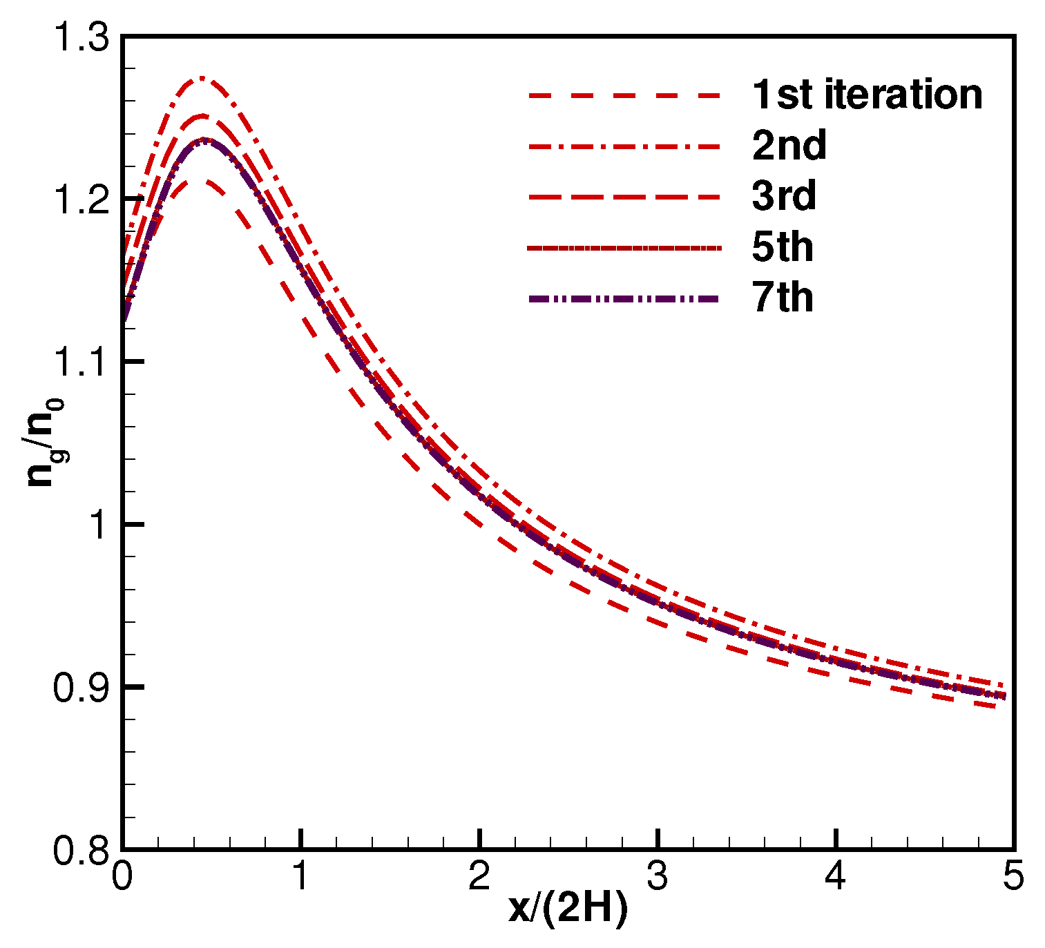
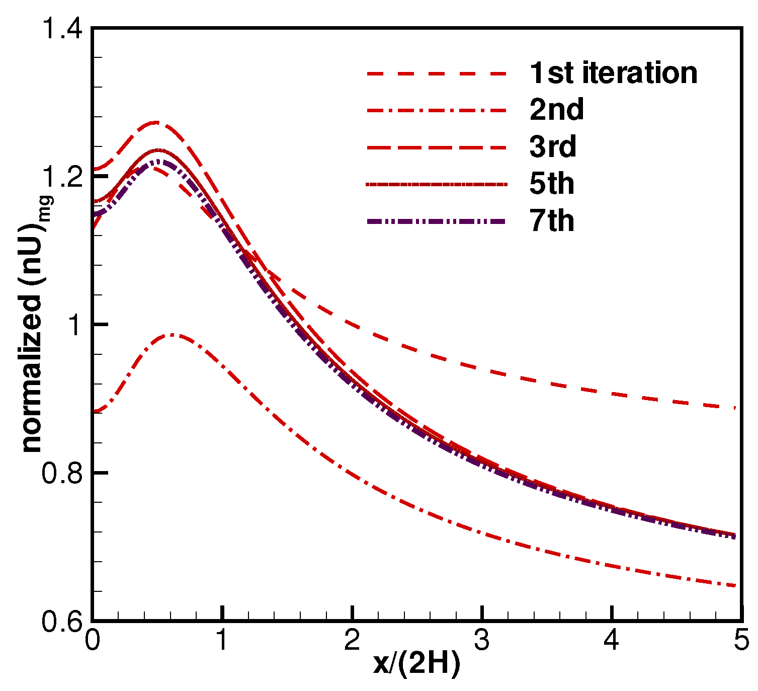
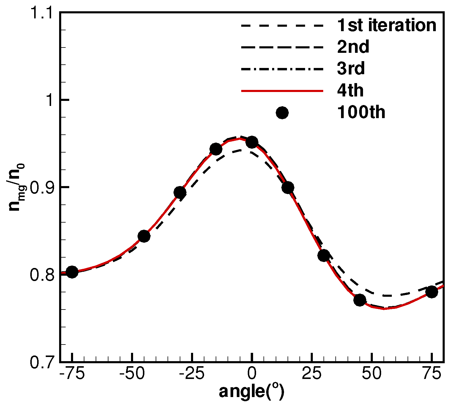
3.2. Test Cases and Discussions

A test case is presented here to demonstrate the procedure. The jet and background flows are assumed as argon with the following parameters: $n_b/n_0=0.8$, $S_0=1.2$, $S_b=0.8$, ${\alpha }_0={45}^{\circ }$, $T_0=200$ Kelvin and $T_b=300$ Kelvin. The number density at the jet exit is $n_0=1\times {10}^{10}$ $m^{-3}$, and it is used as a reference to normalize the background density. Those seven numbers are selected at random for demonstration.

Table 1. Test Parameters: $n_0=1.0$ (non-dimensionalized), $S_0=1.2$, $n_b/n_0=0.8$, $S_b=0.8$, ${\alpha }_0={45}^{\circ }$, $T_0=200$ Kelvin, $T_b=300$ Kelvin. Number densities and fluxes are normalized by $n_0$ and $n_0\sqrt{2R{T}_0}$.

Point	Angle (${}^{\circ }$)	x (m)	y (m)	${\mathit{n}}_{\mathit{m}}$	${\left(\mathit{nU}\right)}_{\mathit{m}}$	${\left(\mathit{nV}\right)}_{\mathit{m}}$
A	−75	0.776	−2.898	0.803	0.542	0.538
B	−45	2.122	−2.121	0.844	0.586	0.498
C	−30	2.598	−1.500	0.894	0.667	0.472
D	−15	2.898	−0.776	0.944	0.763	0.485
E	0.000	3.000	0.000	0.952	0.785	0.539
F	15	2.898	0.776	0.899	0.691	0.576
G	30	2.598	1.500	0.822	0.561	0.549
H	45	2.122	2.121	0.771	0.497	0.497
I	75	0.776	2.898	0.780	0.532	0.509

shows data for density, number fluxes along the X- and Y-directions, at nine points with a radius of 3 m from the jet exit center, but with different relative angles. The jet exit height is 1 m. The values in Table 1 are assumed as accurate measured data.

The following initial estimated parameters are assumed to start the recover procedure: $n_{0g}=0.6$, $S_{0g}=1.0$, $n_{bg}/n_{0g}=1.2$, $S_{bg}=1.0$, ${\alpha }_{0g}={25}^{\circ }$, $T_{0g}=250$ Kelvin, and $T_{bg}=250$ Kelvin. The following properties are taken from Table 1 and assumed known: number densities at points A, C; number fluxes along the X-direction at points D, E, H; and number fluxes along the Y-directions at points H, I. These values form the right hand side terms for the seven equations: two from Equation (21), three from Equation (22), and two from Equation (23).

Table 2. Parameter convergence histories. True values: $n_0=1.0$ (non-dimensionalized), $S_0=1.2$, $n_b/n_0=0.8$, $S_b=0.8$, ${\alpha }_0={45}^{\circ }$, $T_0=200$ Kelvin, $T_b=300$ Kelvin.

Parameter Names	Initial Values	1st Iteration	2nd	3rd	4th	8th	15th
$n_{0g}$	0.60	0.989	1.007	1.018	1.002	0.999	1.000
$S_{0g}$	1.0	1.175	1.232	1.197	1.205	1.201	1.199
$n_{bg}$	1.2	0.802	0.801	0.799	0.799	0.800	0.799
$S_{bg}$	1.0	0.649	0.697	0.779	0.794	0.800	0.799
${\alpha }_{0g}$	25.0	37.57	46.59	44.99	44.99	44.99	45.00
$T_{0g}$	250.0	220.8	127.1	221.5	178.9	195.3	200.4
$T_{bg}$	250.0	346.7	381.5	306.2	303.9	299.9	300.0

shows the development histories for the absolute values for the seven parameters, as shown, after fifteen iterations, the seven estimated parameters are sufficiently close to the true parameters.

Table 3. Parameter convergence histories: relative corrections.

Relative Errors	Initial Values	1st Iteration	2nd	3rd	4th	8th	15th
${ϵ}_1$	$-40.0\%$	$+64.9\%$	$+1.73\%$	$+1.09\%$	$-1.59\%$	$+0.04\%$	$+3.4\times {10}^{-5}$
${ϵ}_2$	$-16.7\%$	$+17.5\%$	$+4.90\%$	$-2.86\%$	$+0.69\%$	$+0.16\%$	$-1.5\times {10}^{-4}$
${ϵ}_3$	$+50.0\%$	$-33.1\%$	$-0.16\%$	$-0.18\%$	$+0.09\%$	$3.3\times {10}^{-6}$	$-1.8\times {10}^{-7}$
${ϵ}_4$	$+25.0\%$	$-35.1\%$	$+7.46\%$	$+11.8\%$	$+1.96\%$	$0.14\%$	$-1.0\times {10}^{-4}$
${ϵ}_5$	$+45.0\%$	$+50.3\%$	$+24.0\%$	$-3.46\%$	$+0.001\%$	$-0.04\%$	$+3.9\times {10}^{-5}$
${ϵ}_6$	$+40.0\%$	$-11.7\%$	$-42.4\%$	$+74.3\%$	$-19.3\%$	$-5.41\%$	$+5.0\times {10}^{-3}$
${ϵ}_7$	$-16.7\%$	$+38.6\%$	$+10.0\%$	$-19.7\%$	$-0.76\%$	$-0.25\%$	$+1.7\times {10}^{-4}$

shows the parameter convergence histories for ${ϵ}_i$, each of them is correction percentage to the values from the previous iteration. As illustrated, the differences among the guessed and true values are negligible after the fifteen iterations. Figure 15, Figure 16 and Figure 17 show the corresponding developing profiles for the jet centerline number density and number fluxes along the X- and Y-directions. Those profiles are computed with updated parameters. These three figures indicate that after three rounds of iterations, the profiles are actually close to the true profiles. At farfield, the profiles merge into the background flows. As discussed in Section 2, the background flow can distort the jet flowfield patterns significantly, or even create totally opposite trends. Figure 18, Figure 19 and Figure 20 show the corresponding profiles for the number density and number fluxes along the arc $R=3$ m, where the data from Table 1 are presented as solid points. As shown, the convergence develops quite fast, the differences are minor among the results obtained by using the parameters obtained after four and ten iterations. It is reasonable to conclude that by using the parameters obtained at the fifteen iterations, the whole flowfield parameters recovered accurately.

Some discussions are offered at the end of this section.

First, it is interesting to compare how this model and the DSMC simulations can recover the seven parameters from very limited measurements. DSMC simulations must start with specific given parameters, it is reasonable to adopt five values for each of the seven parameters, e.g., $n_{0g1}<n_{0g2}<n_{0g3}<n_{0g4}<n_{0g5}$; $S_{0g1}<...<S_{0g5}$; $n_{bg1}<...<n_{bg5}$; $S_{bg1}<...<S_{bg5}$; ${\alpha }_{0g1}<...<{\alpha }_{0g5}$; $T_{0g1}<...<T_{0g5}$, and $T_{bg1}<...<T_{bg5}$. Then there will be $5^7$ = 78,125 sets of parameter combinations from which to obtain the optimal parameter set, if the DSMC simulations are used. The simulation process may require one or several years. However, if the method developed in this paper is adopted, it may only take 10 seconds, with the same computer. This fact illustrates the significance of this new model.

Secondly, this work presents linearized density, and number fluxes along the X- and Y-directions. Is it feasible to derive expressions for the number fluxes along a radial direction? The answer is affirmative. If the angle is assumed as λ, then Equations (22) and (23) can be combined linearly as:

$$\begin{array}{c}(B_1\cos \lambda +C_1\sin \lambda ){ϵ}_1+(B_2\cos \lambda +C_2\sin \lambda ){ϵ}_2+(B_3\cos \lambda +C_3\sin \lambda ){ϵ}_3+\hfill \\ (B_4\cos \lambda +C_4\sin \lambda ){ϵ}_4+(B_5\cos \lambda +C_5\sin \lambda ){ϵ}_5+(B_6\cos \lambda +C_6\sin \lambda ){ϵ}_6+\hfill \\ (B_7\cos \lambda +C_7\sin \lambda ){ϵ}_7+{\left(n_m{U}_m\right)}_g\cos \lambda +{\left(n_m{V}_m\right)}_g\sin \lambda =n_m{U}_m\cos \lambda +n_m{V}_m\sin \lambda ,\hfill \end{array}$$

(24)

Correspondingly, measurements of the number flux along the radial directions are required to form linear equations.

Thirdly, is it feasible to derive a linearized equation for the temperature from Equation (10) or even one equation for pressure? The answer is affirmative. However, the process is lengthier and final results are more complex. The effort will be more demanding, and is not one concern of this feasibility study. This paper aims to demonstrate the method with simple examples.

Fourthly, what if there are more measured data points? They can help further develop more reasonable models. It is reasonable to assume there are at least two groups of highly rarefied background flows in a vacuum chamber. A group of molecules are from the chamber walls with a room temperature, and the other groups of molecules are from pumps with a low temperature. An advanced but similar model can be developed with four additional parameters for a pump, $n_p$, $S_p$, $T_p$, and ${\alpha }_p$, where subscript “$p$” represents pump related property. There will be a total of 7 + 4 = 11 parameters involved in this new model. The new equations corresponding to Equations (7)–(9) shall include extra four new parameters. Each of the linearized Equations (21)–(23) shall include four extra coefficients. The expressions will be more complex, the effort will be more demanding; however, the procedures are the same as those described in this paper.

Fifthly, these approaches and results are superior than results obtained by using the Buckingham PI theorem. The PI theorem can only determine possible numbers of non-dimensional parameters, and possible parameter combinations. However, the PI theorem can not obtain detailed formulas with all factors explicitly embedded, like Equations (7)–(9).

Sixthly, these new approaches can conveniently explain the reasons for differences among measurements, even for the situation with the same nozzle exit parameters but in different vacuum chambers. Due to the geometry differences (e.g., distances and relative angles from the pumps) among ground vacuum chambers, or within the same chamber but different plume firing directions, the background parameters (e.g., the relative angle ${\alpha }_0$ ) may vary. The measurements may be quite different because they are actually for the mixture of jet and background flows, not only for the jet. With these new approaches presented in this paper, the recovered jet parameters $(n_0,U_0,T_0)$ shall be almost identically or quite close. It is also feasible to determine some special chamber characters for a ground vacuum chamber by performing extensive experimental tests and analysis, or even develop general guidelines applicable to many ground vacuum chambers.

Probably the most important question is, can the approaches applicable to more realistic problems, e.g., dilute neutral gas with collisions, or even dilute plasma flows? For the first problem to determine the mixed flowfield with given parameters, simple DSMC or Particle-In-Cell simulations can be performed, or the analytical results from this study can be used for crude approximations. For the second problem to recover the flow parameters from limited measurements, the same recovery procedure presented in this paper, can be applied first by assuming the flow is collisionless neutral or plasma flows. A set of 7 parameters can be recovered. The true parameters must be within the neighborhood of these recovered parameters in the parameter space. This is because the jet and background flows are assumed dilute and weak. A few more particle simulations, either DSMC (for collisional neutral gas), or DSMC+PIC (Particle-In-Cell) (for dilute plasma flows), with parameters from the neighborhood region can lead to the most close parameter set. It is feasible to offset these seven recovered parameters, e.g., each by $\pm 10\%$, then there are $2^7=128$ sets of parameters, with which DSMC or DSMC/PIC simulations can be performed and they may yield more accurate results. By doing this, the simulation amount can reduce by a factor of $78125/128=610$ times.

In this end, it shall be emphasized that the methods from this work do not intend to replace DSMC and any Computational Fluid Dynamics (CFD) simulations, instead, they can help simulations by providing a proper starting point, and significantly reducing the amount of work by narrowing down the parameter ranges. Similarly, this work does not compare the differences among existing experimental methods, nor intends to propose a new experimental method. Instead, the methods from this paper can help analyze the measurements, and perform proper predictions which may be very difficult to measure.

4. Conclusions

In this paper, recent feasibility study results on investigating rarefied background flow effects on a weak jet are presented. The work includes two parts: (1) quantify the background flow or facility effects on a weak jet; and (2) more importantly, recover the related parameters from limited measurements, and with these recovered parameters, the whole flowfield can be recovered, by applying Equations (7)–(11).

First a gaskinetic model is proposed to study collisionless jet and rarefied background flow interactions, in Section 2. New formulas are derived and they accurately capture the combined mixture flowfield. Numerical simulations with the DSMC method were performed and the results validated these new formulas. Based on these new formulas, discussions on the finite background flow effects are offered. It illustrates that background flows may have significant adverse effects on the primary jet flows. Equations (2)–(10) accurately quantify the background facility effects on the jet flowfield, e.g., a change of percentages. All physical factors are explicitly included in these formulas, and a quick glance or evaluation can allow us to understand the roles that a specific non-dimensional parameter plays in the results. Equations (19)–(13) present examples of potential impacts from background flow on EP devices’ performances.

The second part of this paper concentrates on the problem along the opposite direction. Based on the new formulas in Section 2, small perturbation methods are applied with several linearization processes. The analysis yields complex coefficients for linear algebraic equations to solve for the seven parameters characterizing the jet and background flows. An iteration method is developed by first assuming specific values for the seven parameters, and the Gaussian elimination method is used to solve for the deviations. The guessed values are updated after each iteration, until acceptable minor differences among the updated and the measured flowfield densities and/or number fluxes are obtained. To summarize, from as fewer as seven measurements, this new and unique procedure can recover the whole flowfield.

These problems and work are fundamental, the new formulas are for the mixtures with several non-dimensional parameters characterizing the primary and background flows. Analytical solutions can tell at a glance how various physical attributes may affect an answer, or where certain features may dominate a portion of a domain of interest. The ability to produce approximate answers quickly is a tremendous advantage when having to perform a parametric study efficiently. Even though their formats are complex and need computers to evaluate, the evaluation speed is fast for collisionless flows, and no DSMC simulations are needed. Only seven measured data are required to recover the whole flowfield. The performance of convergence speed and accuracy are truly remarkable. For dilute collisional neutral or plasma flows, similar approaches can be developed and they can reduce the amount of simulations by a factor of a few hundreds or even thousands.

In summary, the work is unique, it proposed new analytical approaches to analyze dilute background flow or facility effects on weak jets. Applications may apply for EP device test or performance estimations in a space environment or tested in a vacuum chamber. These new methods can be supplemental tools which are far more fast and inexpensive, to help experimental test and numerical simulations.

References

1. Sanna, G.; Tomassetti, G. Introduction to Molecular Beams Gas Dynamics; Imperial College Press: London, UK, 2005. [Google Scholar]
2. Maev, R.; Leshchynsky, V. Introduction to Low Pressure Gas Dynamic Spray; Wiley-Vch: Weinheim, Germany, 2008. [Google Scholar]
3. Hastings, D.; Garrett, H. Spacecraft-Environment Interactions; Cambridge University Press: Cambridge, UK, 1996. [Google Scholar]
4. Simons, G.A. Effects of nozzle boundary layers on rocket exhaust plumes. AIAA J. 1972, 10, 1534–1535. [Google Scholar] [CrossRef]
5. Jian, H.; Chu, Y.; Cao, H.; Cao, Y.; He, X.; Xia, G. Three-dimensional IFE-PIC numerical simulation of background pressure’s effect on accelerator grid impingement current for ion optics. Vacuum 2015, 116, 130–138. [Google Scholar] [CrossRef]
6. Byers, C.C.; Dankanich, J.W. A review of facility effects on Hall effect thrusters. In Proceedings of the 31st International Electric Propulsion Conference, Ann Arbor, MI, USA, 20–24 September 2009. IEPC-2009-076.
7. Gildea, S.R.; Sanchez, M.M.; Nakles, M.R.; Hargus, W.A. Experimentally characterizing the plume of a divergent cusped field thruster. In Proceedings of the 31st International Electric Propulsion Conference, Ann Arbor, MI, USA, 20–24 September 2009. AFRL-RZ-ED-TP-2009-316.
8. Dankanich, J.W.; Swiatek, M.W.; Yim, T. A step towards electric propulsion testing standards: Pressure measurements and effective pumping speeds. In Proceedings of the48th AIAA/ASME/SAE/ASEE Joint Propulsion Conference and Exhibit, Altanta, GA, USA, 30 July–1 August 2012. AIAA paper 2012-3737.
9. Jones, M.L. Results of large vacuum facility tests of an MPD arc thruster. AIAA J. 1966, 4, 1455–1456. [Google Scholar] [CrossRef]
10. Sovey, J.S.; Mantenieks, M.A. Performance and lifetime assessment of MPD arc thruster technology. In Proceedings of the 24th AIAA/ASME/SAE/ASEE Joint Propulsion Conference, Boston, MA, USA, 11–13 July 1988. AIAA Paper 88-3211.
11. Nakles, M.R.; Hargus, W.A. Background pressure effects on ion velocity distribution within a medium-power Hall thruster. J. Propuls. Power 2011, 27, 737–743. [Google Scholar] [CrossRef]
12. Randolph, T.; Kim, V.; Kozubsky, K.; Zhurin, V.; Day, M. Facility effects on stationary plasma thruster testing. In Proceedings of the 23rd International Electric Propulsion Conference, Seattle, WA, USA, 13–16 September 1993. IEPC-93-93 844.
13. Hofer, R.R.; Peterson, P.Y.; Gallimore, A.D. Characterizing vacuum facility back pressure effects on the performance of a Hall thruster. In Proceedings of the 27th International Electric Propulsion Conference, Pasadena, CA, USA, 15–19 October 2001. IEPC-01-045.
14. Walker, M.L.R.; Gallimore, A.D.; Boyd, I.D.; Cai, C. Vacuum chamber pressure maps of a Hall thruster cold-flow expansion. J. Propuls. Power 2004, 20, 1127–1132. [Google Scholar] [CrossRef]
15. Rovey, J.L.; Walker, M.L.R.; Gallimore, A. Magnetically filtered Faraday probe for measuring the ion current density profile of a Hall thruster. Rev. Sci. Instrum. 2006, 77, 013503. [Google Scholar] [CrossRef] [Green Version]
16. Kamhawi, H.; Huang, W.; Haag, T.; Spektor, R. Investigation of the effects of facility background pressure on the performance and voltage-current characteristics of the high voltage Hall accelerator. In Proceedings of the 50th AIAA/ASME/SAE/ASEE Joint Propulsion Conference 2014, Cleveland, OH, USA, 28–30 July 2014. AIAA Paper 2014-17063.
17. Huang, W.; Kamhawi, H.; Hagg, W. Facility effect characterization test of NASA’s HERMes Hall thruster. In Proceedings of the 52nd AIAA/SAE/ASEE Jointed Propulsion Conference, Salt Lake City, UT, USA, 25–27 July 2016. AIAA paper 2016-4842.
18. Li, X.; Zhang, T.; Jia, Y.; Chen, J. Numerical simulations of space background pressure effects on stability parameters for ion thruster grids. Vac. Cryog. 2012, 18, 71–76. Available online: http://www.cqvip.com/qk/95890x/201202/43092185.html (accessed on 1 December 2016). (In Chinese)[Google Scholar]
19. Yim, J.; Burt, J. Characterization of vacuum facility background gas through simulation and considerations for electric propulsion ground testing chambers. In Proceedings of the 51st AIAA/SAE/ASEE Joint Propulsion Conference, Orlando, FL, USA, 27–29 July 2015. AIAA paper 2015-3825.
20. Bird, G. Molecular Gas Dynamics and the Direct Simulation of Gas Flows, 2nd ed.; Clarendon Press: Oxford, UK, 1994. [Google Scholar]
21. Narasimha, R. Collisionless expansion of gases into vacuum. J. Fluid Mech. 1962, 12, 294–308. [Google Scholar] [CrossRef]
22. Liepmann, H.W. Gas kinetics and gasdynamics of orifice flow. J. Fluid Mech. 1961, 10, 65–79. [Google Scholar] [CrossRef]
23. Cai, C.; Zou, C. Gaskinetic solutions for high Knudsen number planar jet impingement flows. Commun. Comput. Phys. 2013, 14, 960–978. [Google Scholar] [CrossRef]
24. Cai, C.; Huang, X. High speed rarefied round jet impingement flows. AIAA J. 2012, 50, 2908–2911. [Google Scholar] [CrossRef]
25. Cai, C.; Khasawneh, K. Collisionless gas flows over a flat cryogenic pump plate. J. Vac. Sci. Technol. A 2009, 27, 601–610. [Google Scholar] [CrossRef]
26. Cai, C.; Boyd, I.D.; Sun, Q. Free molecular background flow in a vacuum chamber equipped with two-sided pumps. J. Vac. Sci. Technol. A 2006, 24, 9–19. [Google Scholar] [CrossRef]
27. Cai, C.; Boyd, I.D.; Sun, Q. Free molecular flows between two plates equipped with pumps. J. Thermophys. Heat Transf. 2007, 21, 95–104. [Google Scholar] [CrossRef]
28. Noller, H.G. Approximate calculation of expansion of gas from nozzles into high vacuum. J. Vac. Sci. Technol. 1966, 6, 202. [Google Scholar] [CrossRef]
29. Liu, H.; Cai, C.; Zou, C. An object-oriented implementation of the DSMC method. Comput. Fluids 2012, 57, 65–75. [Google Scholar] [CrossRef]
Figure 1. Problem illustration.
Aerospace 04 00005 g001
Figure 2. Velocity phases. (a) Jet; (b) Background flow. K J u = M U b u = θ 1 , I J u = L U b u = θ 2 .
Aerospace 04 00005 g002
Figure 3. Nondimensional density contours for the jet/background mixture, n b / n 0 = 0.2 , S 0 = 2.0 , α 0 = 45 , S b = 1.0 , T 0 = 200 Kelvin, and T b = 300 Kelvin. Red: analytical, black: direct simulation Monte Carlo (DSMC).
Aerospace 04 00005 g003
Figure 4. Nondimensional U-velocity component contours for the jet/background mixture, n b / n 0 = 0.2 , S 0 = 2.0 , α 0 = 45 , S b = 1.0 , T 0 = 200 Kelvin, and T b = 300 Kelvin. Red: analytical, black: DSMC.
Aerospace 04 00005 g004
Figure 5. Nondimensional V-velocity component contours for the jet/background mixture, n b / n 0 = 0.2 , S 0 = 2.0 , α 0 = 45 , S b = 1.0 , T 0 = 200 Kelvin, and T b = 300 Kelvin. Red: analytical, black: DSMC.
Aerospace 04 00005 g005
Figure 6. Nondimensional translational temperature contours for the jet/background mixture, n b / n 0 = 0.2 , S 0 = 2.0 , α 0 = 45 , S b = 1.0 , T 0 = 200 Kelvin, and T b = 300 Kelvin. Red: analytical, black: DSMC.
Aerospace 04 00005 g006
Figure 7. Nondimensional pressure contours for the jet/background mixture, n b / n 0 = 0.2 , S 0 = 2.0 , α 0 = 45 , S b = 1.0 , T 0 = 200 Kelvin, and T b = 300 Kelvin. Red: analytical, black: DSMC.
Aerospace 04 00005 g007
Figure 8. Background flow effects on centerline number density profiles for the mixture, n b / n 0 = 0.2 , S 0 = 2.0 , S b = 1.0 , T 0 = 200 Kelvin, and T b = 300 Kelvin.
Aerospace 04 00005 g008
Figure 9. Background flow effects on centerline u-velocity component profiles for the mixture, n b / n 0 = 0.2 , S 0 = 2.0 , S b = 1.0 , T 0 = 200 Kelvin, and T b = 300 Kelvin.
Aerospace 04 00005 g009
Figure 10. Background flow effects on centerline temperature profiles for the mixture, n b / n 0 = 0.2 , S 0 = 2.0 , S b = 1.0 , T 0 = 200 Kelvin, and T b = 300 Kelvin.
Aerospace 04 00005 g010
Figure 11. Background flow effects on centerline pressure profiles for the mixture, n b / n 0 = 0.2 , S 0 = 2.0 , S b = 1.0 , T 0 = 200 Kelvin, and T b = 300 Kelvin.
Aerospace 04 00005 g011
Figure 12. Background flow effects on the local number flux (normalized by n 0 2 R T 0 , along r / ( 2 H ) = 4 . , n b / n 0 = 0.5 , S 0 = 0.2 , S b = 0.1 , T 0 = 200 Kelvin, and T b = 300 Kelvin.
Aerospace 04 00005 g012
Figure 13. Illustration for different number flux across different curves.
Aerospace 04 00005 g013
Figure 14. Background flow effects on the total number flux rate across different radius (normalized by n 0 2 R T 0 ), within angle span 75 < θ < 75 , n b / n 0 = 0.5 , S 0 = 0.2 , S b = 0.1 , T 0 = 200 Kelvin, and T b = 300 Kelvin.
Aerospace 04 00005 g014
Figure 15. Test case: mixture centerline density profile development history.
Aerospace 04 00005 g015
Figure 16. Test case: mixture centerline number flux n U / ( n 0 2 R T 0 ) profile development history.
Aerospace 04 00005 g016
Figure 17. Test case: mixture centerline number flux n V / ( n 0 2 R T 0 ) profile development history.
Aerospace 04 00005 g017
Figure 18. Test case: mixture density profile development history, along R = 3 m.
Aerospace 04 00005 g018
Figure 19. Test case: mixture number flux n U / ( n 0 2 R T 0 ) profile development history, along R = 3 m.
Aerospace 04 00005 g019
Figure 20. Test case: mixture number flux n V / ( n 0 2 R T 0 ) profile development history, along R = 3 m.
Aerospace 04 00005 g020