
Electromagnetic Simulation and Alignment of Dual-Polarized Array Antennas in Multi-Mission Phased Array Radars †


Abstract
:
1. Introduction
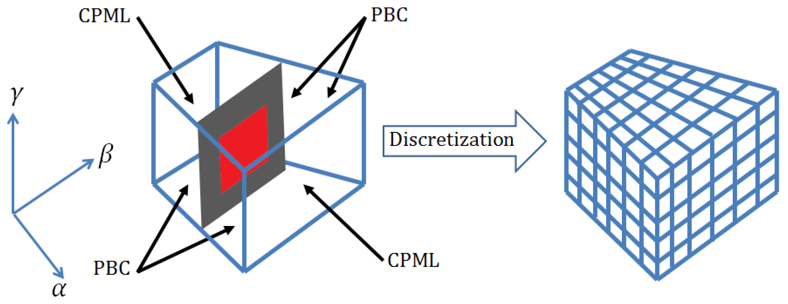
2. Theory
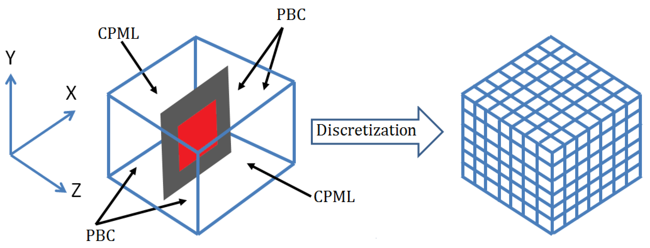
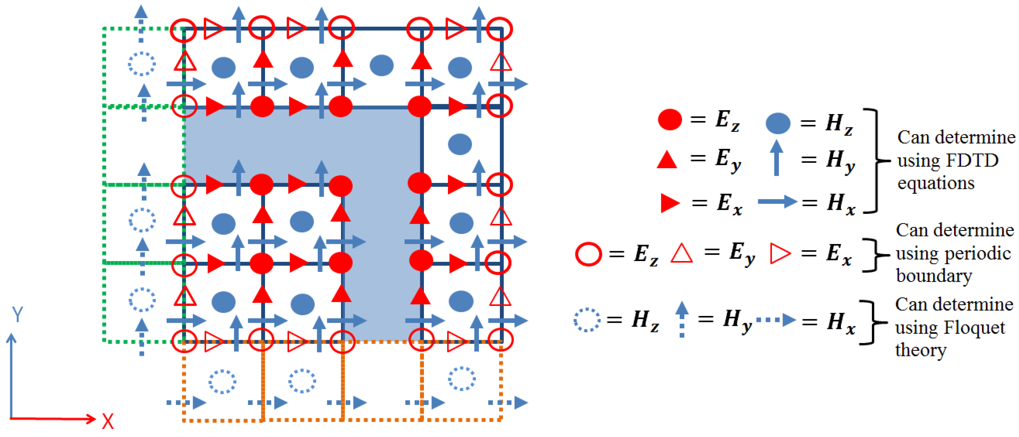
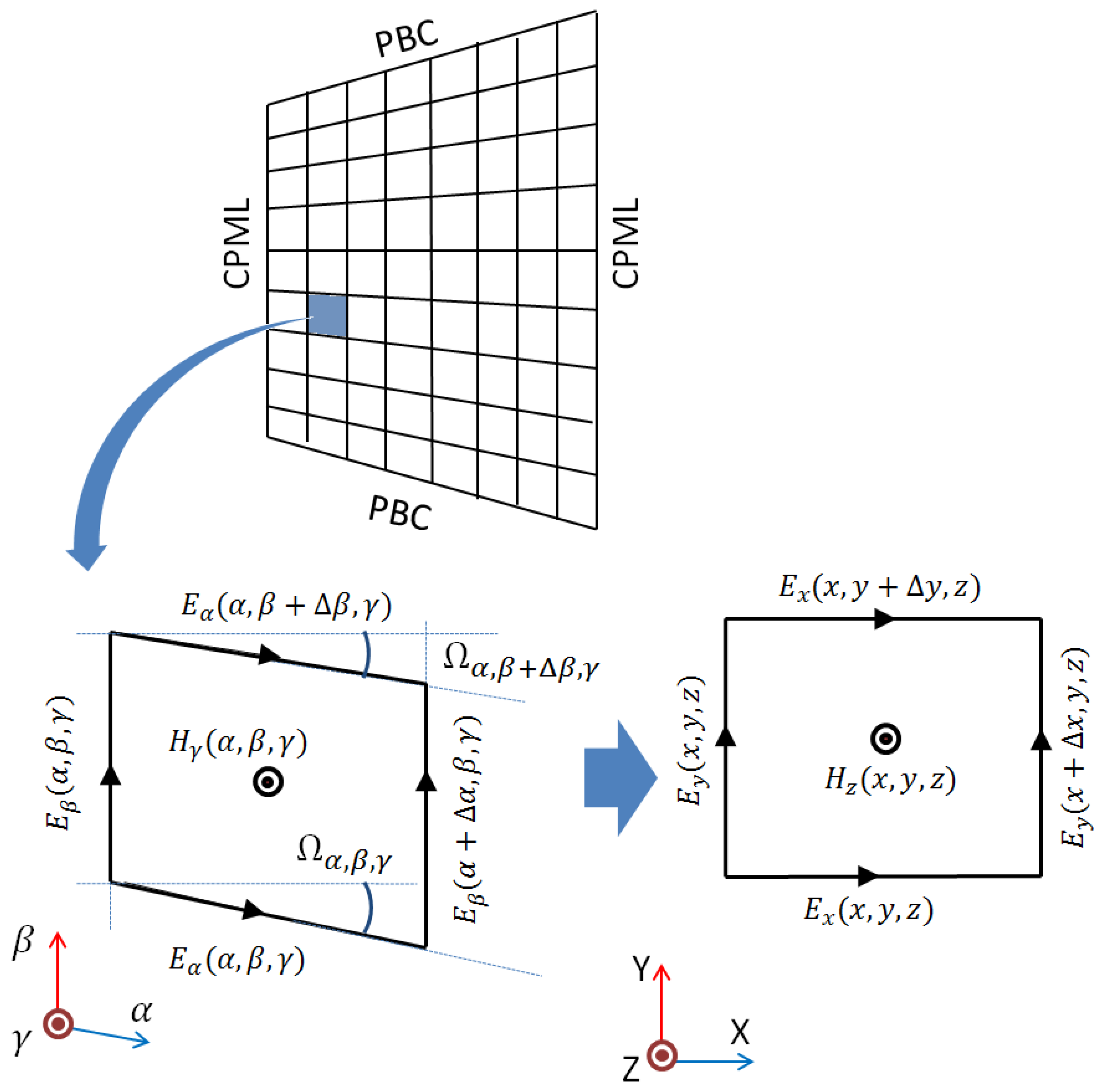
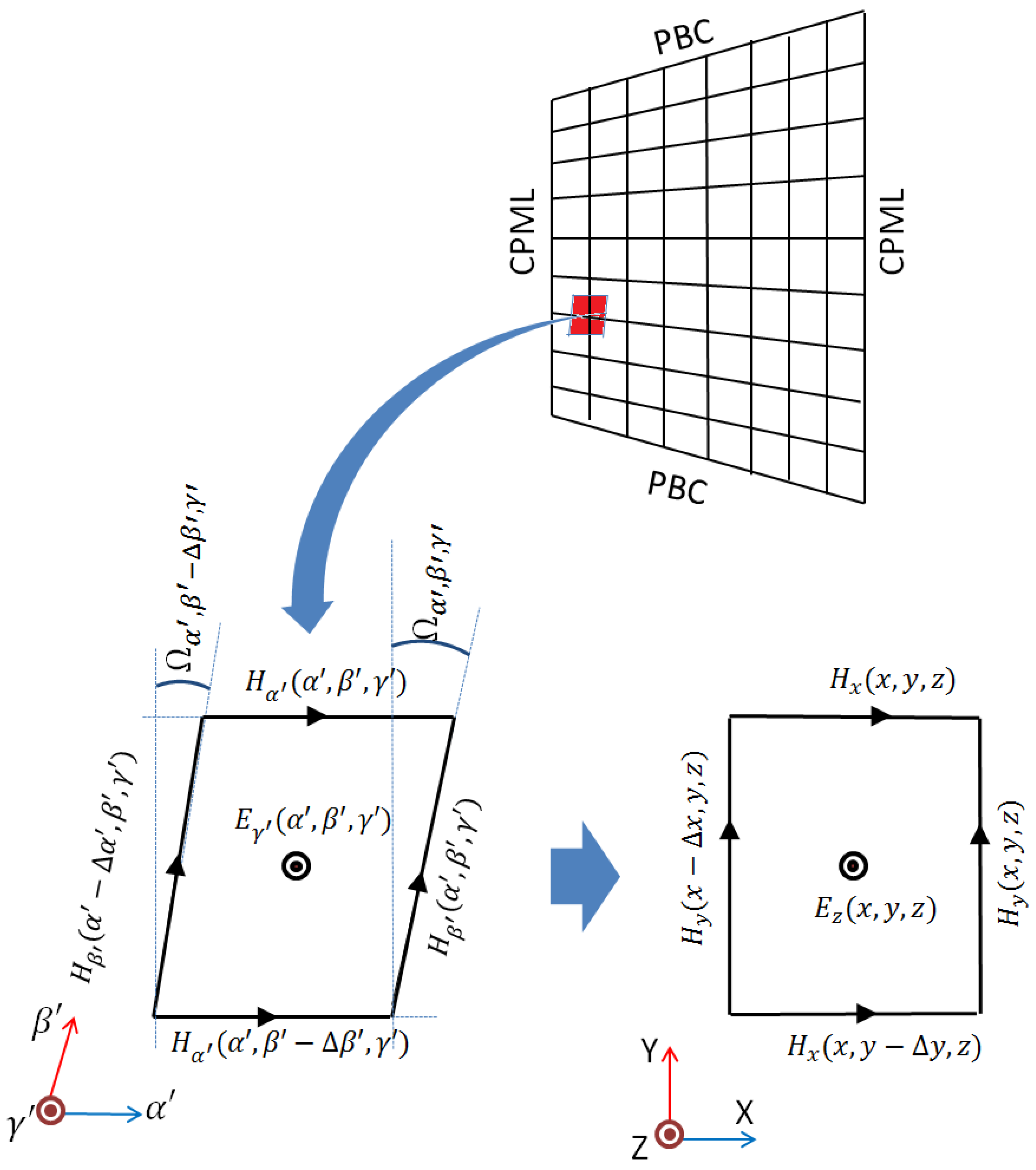
2.1. Rectangular Grid
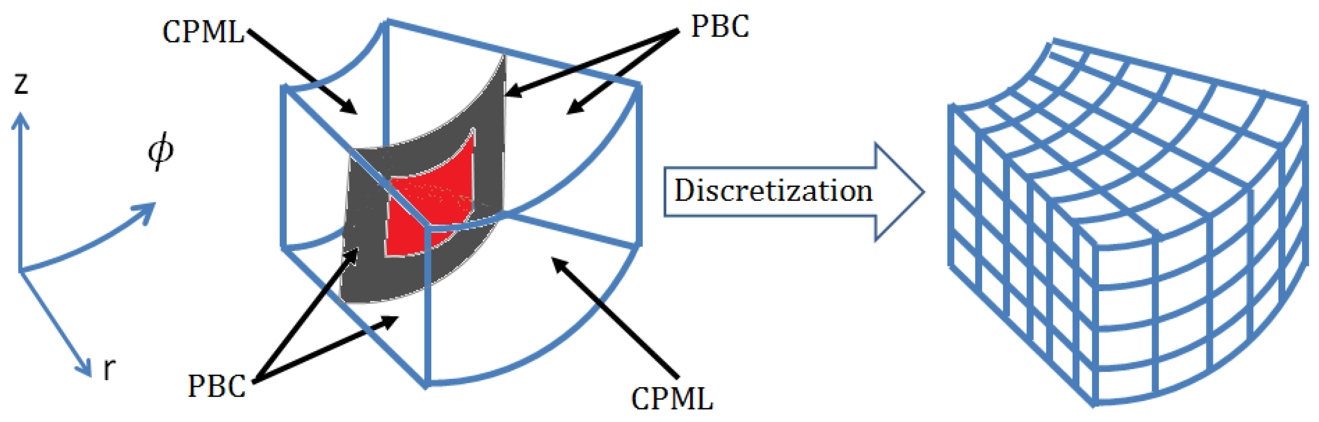
2.2. Cylindrical Grid
2.2.1. Periodicity in the Direction
2.2.2. Periodicity in the Direction
2.2.3. At the Corners
2.3. Nonorthogonal Grid
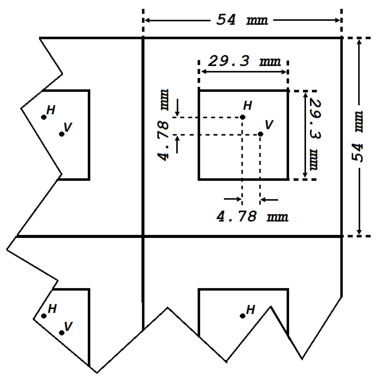
3. Simulation of Active Element Patterns
3.1. Computational Load
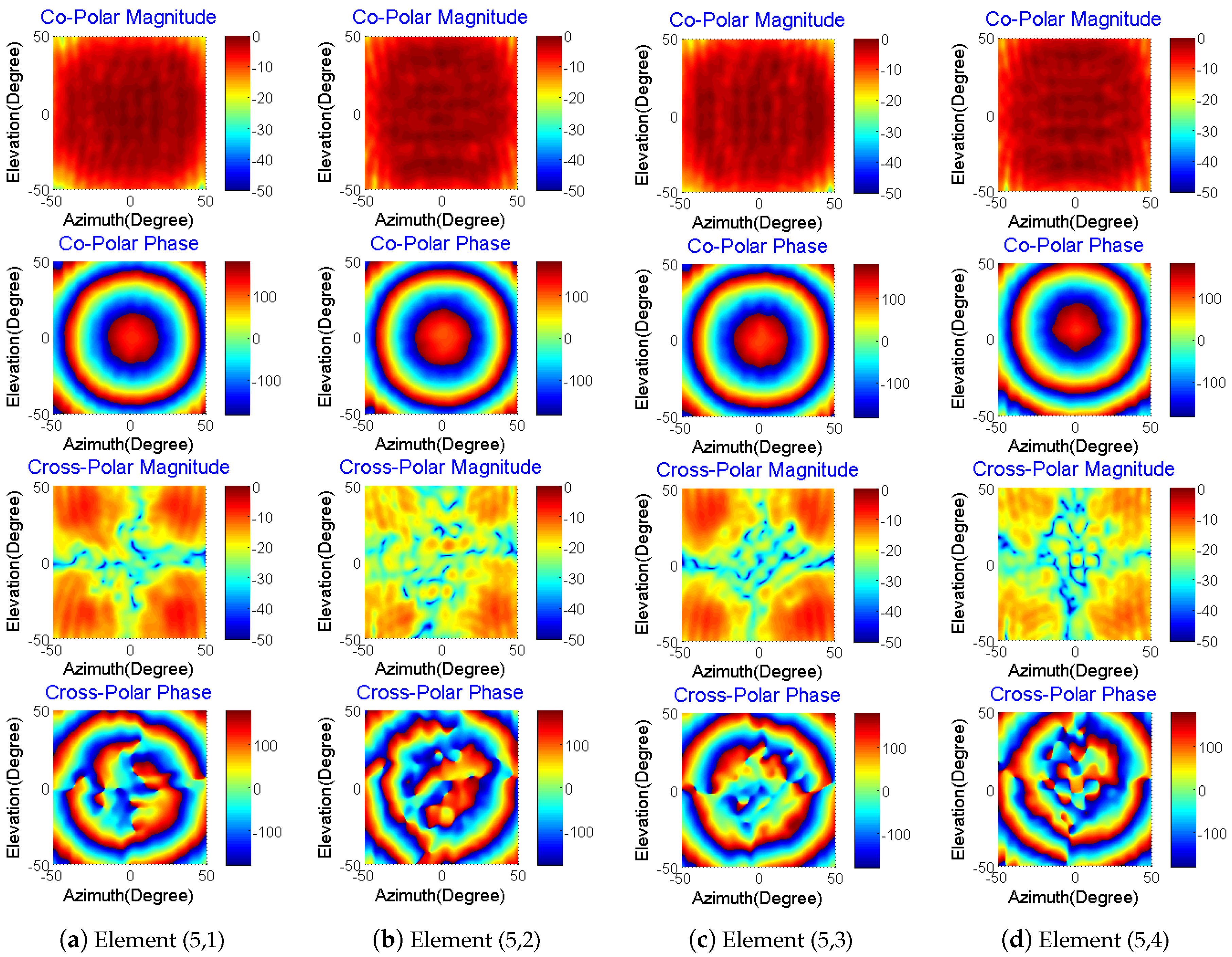
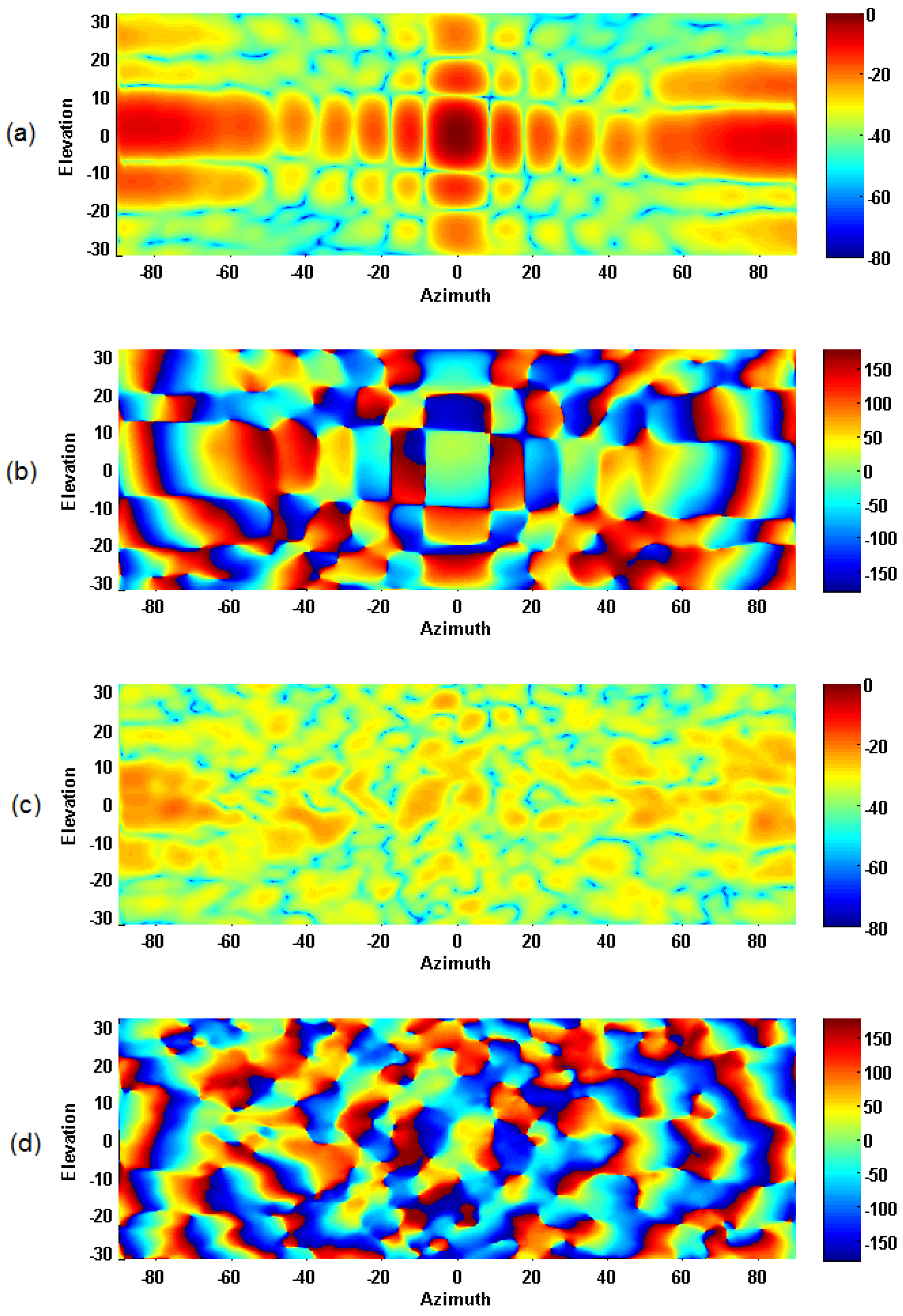
3.2. Example Results of Simulated AEP
4. Measurements of Active Element Patterns
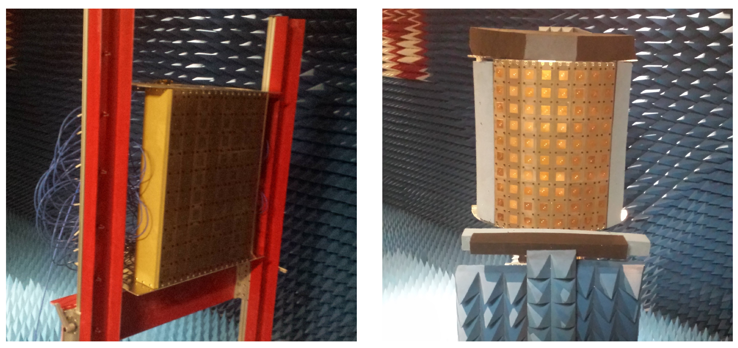
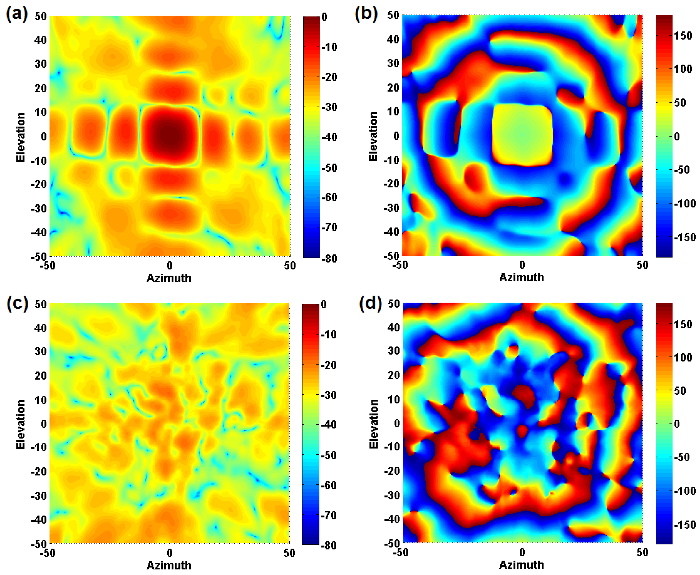
4.1. Planar Array Example Measurement Results
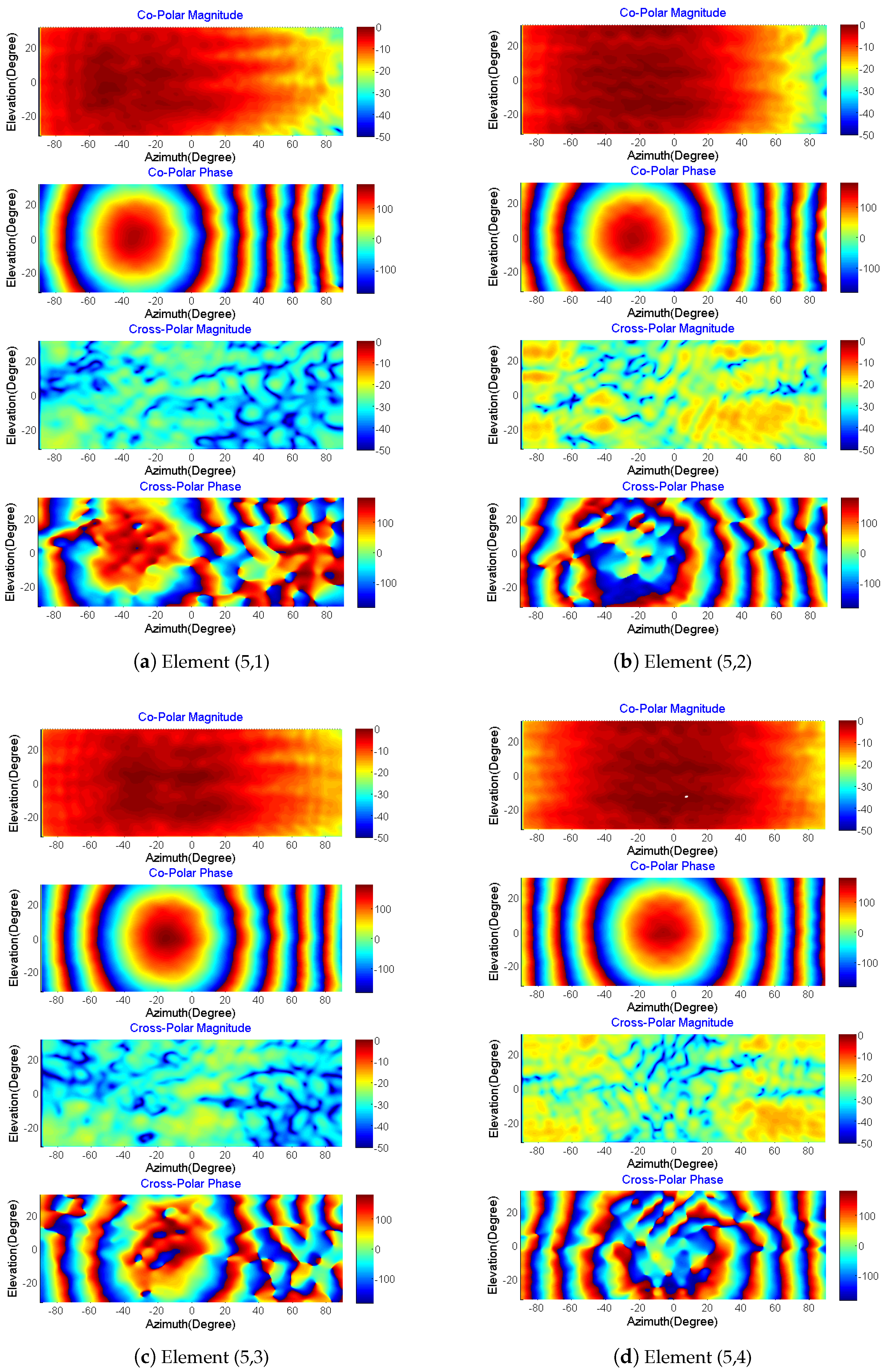
4.2. Faceted-Cylindrical Array Example Measurement Results
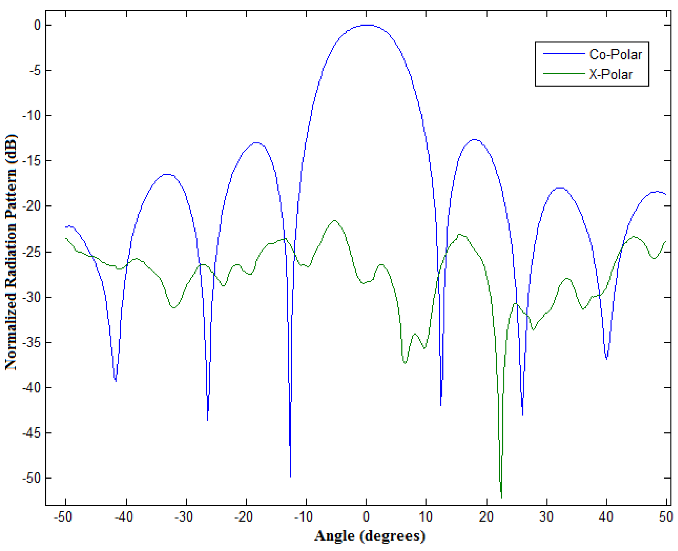
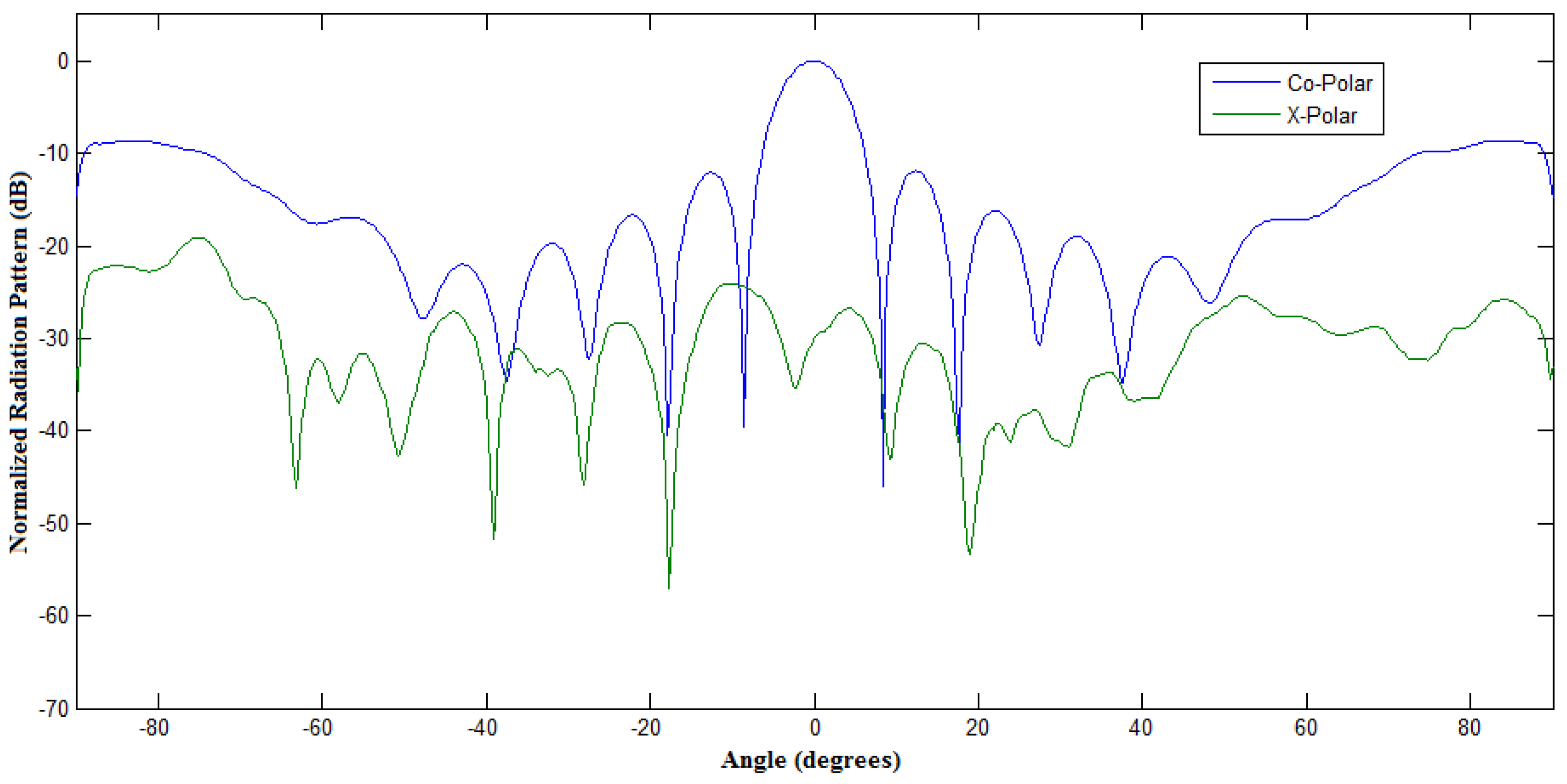
5. Generation of The Array Pattern from Measured AEP
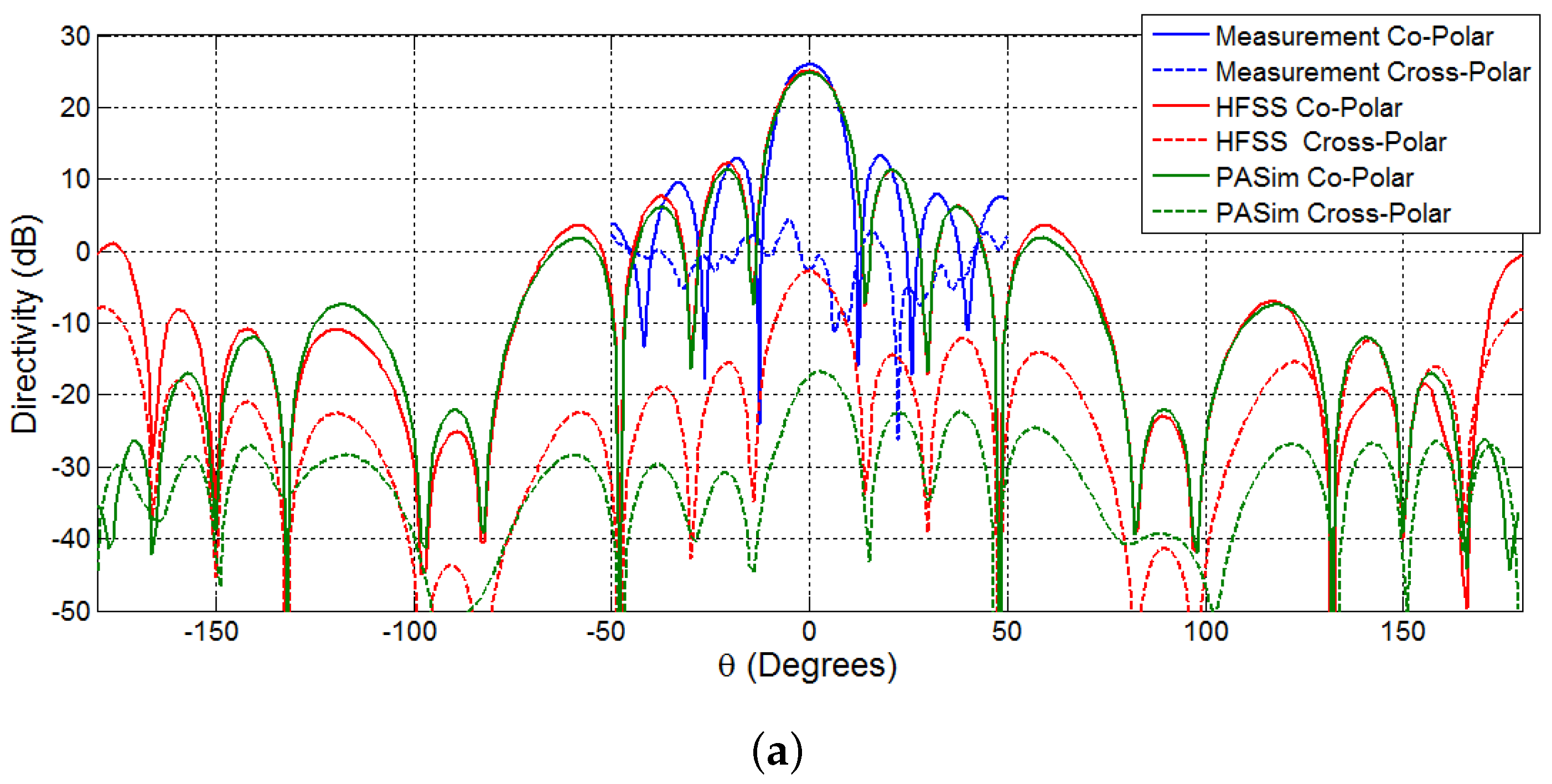
5.1. The Planar Array (Case I)
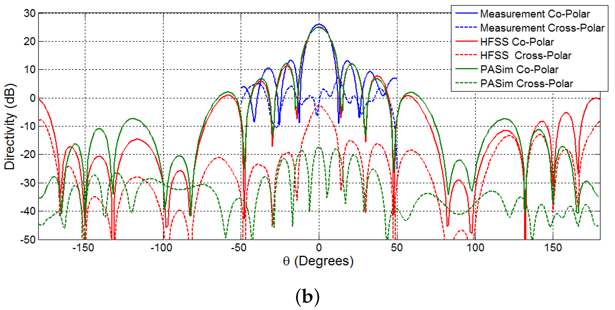
5.2. The Faceted-Cylindrical Array (Case II)
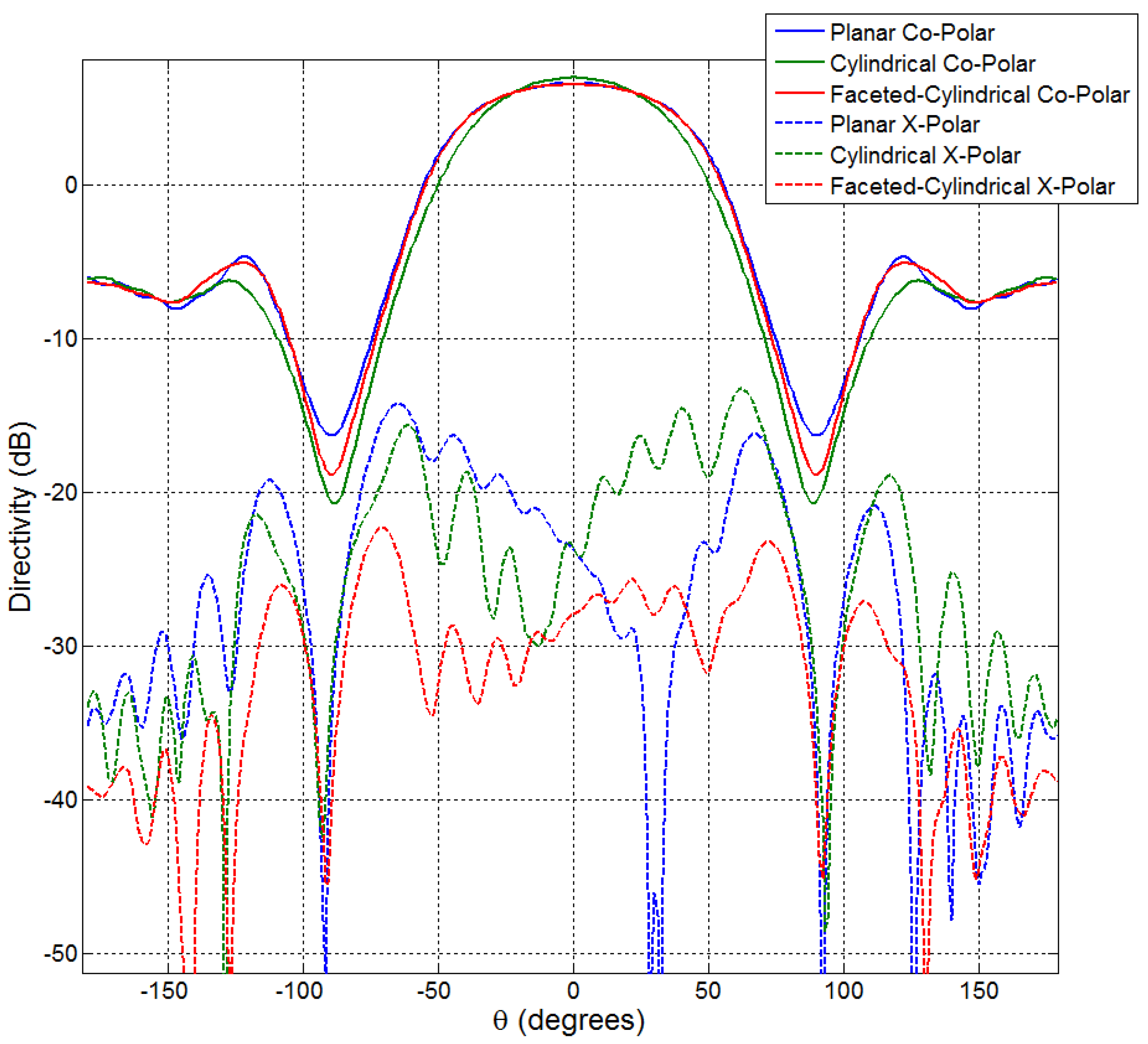
5.3. Comparison of the Results of the Planar Array vs. the Facet Cylindrical Array
6. Large Finite Array Antennas
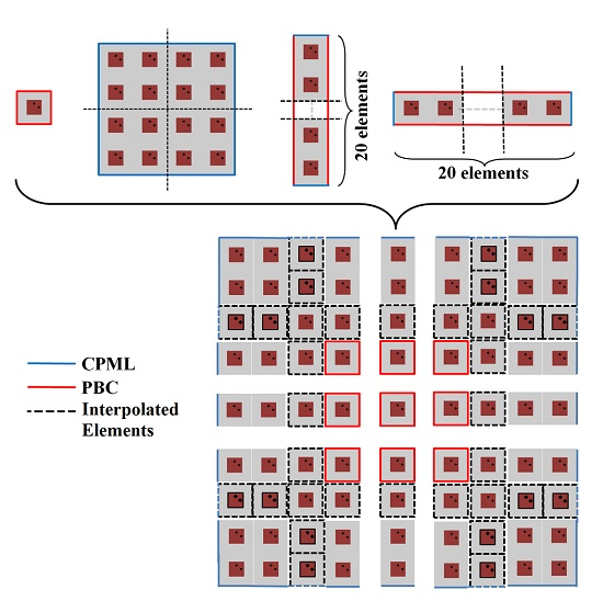
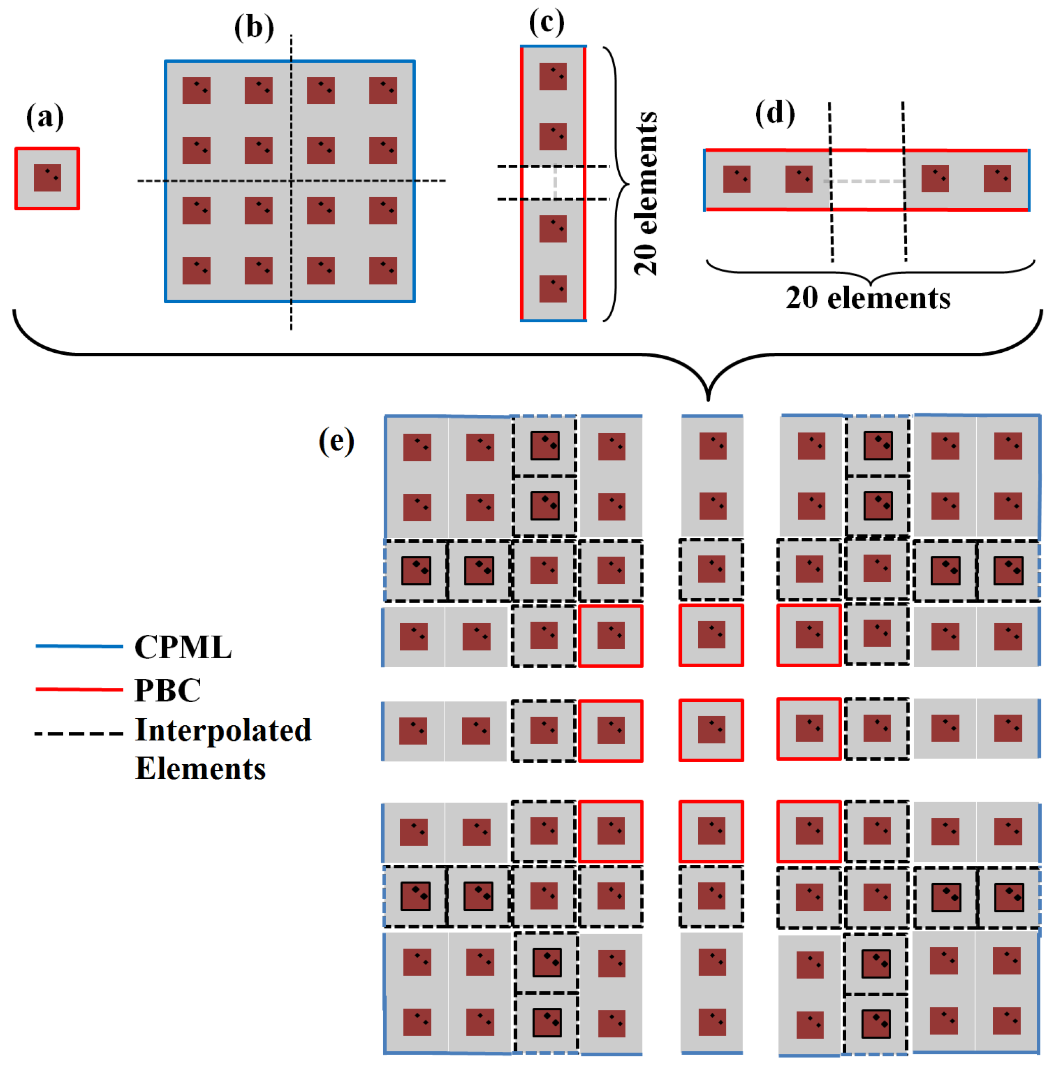
6.1. Near-Field Aperture Merging Technique
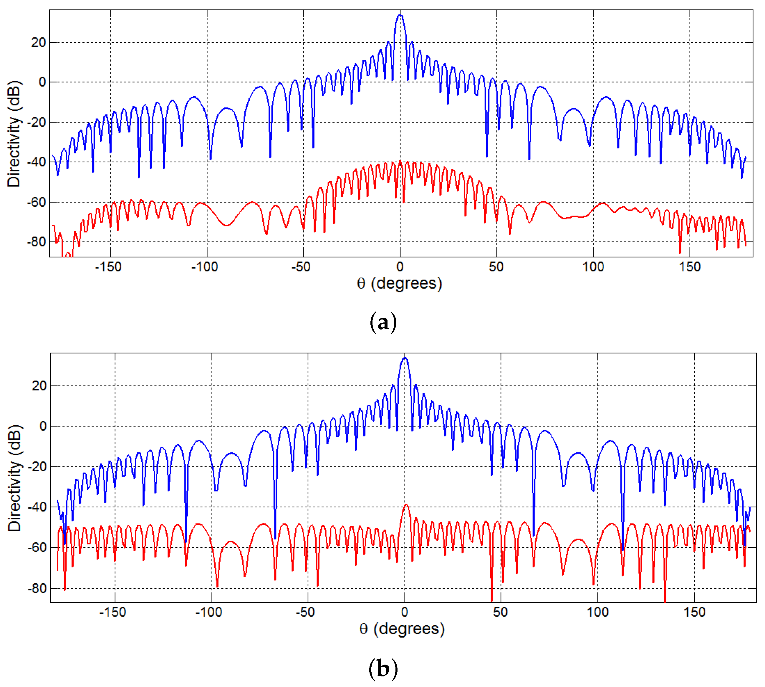
6.2. Simulation of Larger Scale Cylindrical and Facet Arrays
6.3. Simulation of Larger Scale Planar Arrays
7. Summary and Conclusions
Acknowledgments
Author Contributions
Conflicts of Interest
Abbreviations
| EM | Electromagnetic |
| PASim | Phased Array Simulator |
| FDTD | Finite Difference Time Domain |
| CPAD | Configurable Polarimetric Array Demonstrator |
| AEP | Active Element Pattern |
| MPAR | Multi-Functional Phased Array Radar |
| PAA | Phased Array Antenna |
| PBC | Periodic Boundary Condition |
| CPML | Convolutional Perfectly Matched Layer |
| NF | Near-Field |
| CPU | Central Processing Unit |
| RAM | Random-Access Memory |
| HFSS | High Frequency Structural Simulator |
| GPGPU | General-Purpose Graphic Processing Unit |
| NOAA | National Oceanic and Atmospheric Administration |
| NSSL | National Severe Storms Laboratory |
Appendix A. FDTD Updating Equation Based on the Cylindrical Grid in an Anisotropic Material
Appendix B. FDTD Updating Equation Based on the Nonorthogonal Grid in an Isotropic Material
References
- Stutzman, W.; Thiele, G. Antenna Theory and Design; John Wiley & Sons: Hoboken, NJ, USA, 2012. [Google Scholar]
- Balanis, C. Antenna Theory: Analysis and Design; John Wiley & Sons: Hoboken, NJ, USA, 2005. [Google Scholar]
- Fenn, A. Adaptive Antennas and Phased Arrays for Radar and Communications; Artech House: Norwood, MA, USA, 2007. [Google Scholar]
- Herd, J.; Carlson, D.; Duffy, S.; Weber, M.; Brigham, G.; Rachlin, M.; Weigand, C. Multifunction Phased Array Radar (MPAR) for Aircraft and Weather Surveillance. In Proceedings of the 2010 IEEE Radar Conference, Washington, DC, USA, 10–14 May 2010; pp. 945–948.
- Weber, M.; Cho, J.; Herd, J.; Flavin, J.; Benner, W.; Torok, G. The next-generation multimission US surveillance radar network. Bull. Am. Meteorol. Soc. 2007, 88, 1739. [Google Scholar] [CrossRef]
- Karimkashi, S.; Zhang, G. A dual-polarized series-fed microstrip antenna array with very high polarization purity for weather measurements. IEEE Trans. Antennas Propag. 2013, 61, 5315–5319. [Google Scholar] [CrossRef]
- Munk, B. Finite Antenna Arrays and FSS; John Wiley & Sons: Hoboken, NJ, USA, 2003. [Google Scholar]
- Perera, S.; Pan, Y.; Zhao, Q.; Zhang, Y.; Zrnic, D.; Doviak, R. A fully reconfigurable polarimetric phased array testbed: Antenna integration and initial measurements. In Proceedings of the 2013 IEEE International Symposium on Phased Array Systems & Technology, Waltham, MA, USA, 15–18 October 2013.
- Perera, S.; Pan, Y.; Zhang, Y.; Yu, X.; Zrnic, D.; Doviak, R. A fully reconfigurable polarimetric phased array antenna testbed. Int. J. Antennas Propag. 2014, 2014, 439606. [Google Scholar] [CrossRef]
- Perera, S.; Zhang, Y. Dual Polarized Phased Array Antenna Simulation Using Optimized FDTD Method With PBC. In Proceedings of the 37th Conference on Radar Meteorology, Norman, OK, USA, 14–18 September 2015.
- Perera, S.; Zhang, Y.; Zrnic, D.; Doviak, R. Scalable EM Simulation and Validations of Dual-Polarized Phased Array Antennas for MPAR. In Proceedings of the 2016 IEEE International Symposium on Phased Array Systems & Technology, Waltham, MA, USA, 18–21 October 2016.
- Josefsson, L.; Patrik, P. Conformal Array Antenna Theory and Design; John Wiley & Sons: Hoboken, NJ, USA, 2006; Volume 29. [Google Scholar]
- Yee, K. Numerical solution of initial boundary value problems involving Maxwell’s equations in isotropic media. IEEE Trans. Antennas Propag. 1966, 14, 302–307. [Google Scholar]
- Elsherbeni, A.; Demir, V. The Finite Difference Time Domain Method for Electromagnetics: With MATLAB Simulations; SciTech Publishing: Raleigh, NC, USA, 2016. [Google Scholar]
- Taflove, A.; Hagness, S. Computational Electrodynamics; Artech House Publishers: Norwood, MA, USA, 2000. [Google Scholar]
- Fulton, C.; Mirkamali, A. A Computer-Aided Technique for the Analysis of Embedded Element Patterns of Cylindrical Arrays [EM Programmer’s Notebook]. IEEE Antennas Propag. Mag. 2015, 57, 132–138. [Google Scholar] [CrossRef]
- ElMahgoub, K.; Yang, F.; Elsherbeni, A.; Demir, V.; Chen, J. FDTD analysis of periodic structures with arbitrary skewed grid. IEEE Trans. Antennas Propag. 2010, 58, 2649–2657. [Google Scholar] [CrossRef]
- Turner, G.; Christodoulou, C. FDTD analysis of phased array antennas. IEEE Trans. Antennas Propag. 1999, 47, 661–667. [Google Scholar] [CrossRef]
- Chen, Y.; Liu, Y.; Chen, B.; Zhang, P. A cylindrical higher-order FDTD algorithm with PML and quasi-PML. IEEE Trans. Antennas Propag. 2013, 61, 4695–4704. [Google Scholar] [CrossRef]
- He, J.; Liu, Q. A nonuniform cylindrical FDTD algorithm with improved PML and quasi-PML absorbing boundary conditions. IEEE Trans. Geosci. Remote Sens. 1999, 37, 1066–1072. [Google Scholar]
- Liu, Y.; Chen, Y.; Chen, B.; Xu, X. A cylindrical MRTD algorithm with PML and quasi-PML. IEEE Trans. Microw. Theory Tech. 2013, 61, 1006–1017. [Google Scholar] [CrossRef]
- Teixeira, F.; Chew, W. PML-FDTD in cylindrical and spherical grids. IEEE Microw. Guided Wave Lett. 1997, 7, 285–287. [Google Scholar] [CrossRef]
- Bhattacharyya, A. Phased Array Antennas: Floquet Analysis, Synthesis, BFNs and Active Array Systems; John Wiley and Sons: Hoboken, NJ, USA, 2006; Volume 179. [Google Scholar]
- Ludwig, A. The definition of cross polarization. IEEE Trans. Antennas Propag. 1973, 21, 116–119. [Google Scholar] [CrossRef]
- Mailloux, R. Phased Array Antenna Handbook; Artech House: Norwood, MA, USA, 2005. [Google Scholar]


© 2017 by the authors. Licensee MDPI, Basel, Switzerland. This article is an open access article distributed under the terms and conditions of the Creative Commons Attribution (CC BY) license ( http://creativecommons.org/licenses/by/4.0/).
Share and Cite
Perera, S.; Zhang, Y.; Zrnic, D.; Doviak, R. Electromagnetic Simulation and Alignment of Dual-Polarized Array Antennas in Multi-Mission Phased Array Radars. Aerospace 2017, 4, 7. https://doi.org/10.3390/aerospace4010007
Perera S, Zhang Y, Zrnic D, Doviak R. Electromagnetic Simulation and Alignment of Dual-Polarized Array Antennas in Multi-Mission Phased Array Radars. Aerospace. 2017; 4(1):7. https://doi.org/10.3390/aerospace4010007
Chicago/Turabian StylePerera, Sudantha, Yan Zhang, Dusan Zrnic, and Richard Doviak. 2017. "Electromagnetic Simulation and Alignment of Dual-Polarized Array Antennas in Multi-Mission Phased Array Radars" Aerospace 4, no. 1: 7. https://doi.org/10.3390/aerospace4010007