Experimental Implementation of a Passive Millimeter-Wave Fast Sequential Lobing Radiometric Seeker Sensor

Abstract

The paper investigates the theory of operation of a passive millimeter-wave seeker sensor using a fast electronic sequential-lobing technique and the experimental validation obtained through laboratory trials. The paper analyzes in detail the theoretical performance of a difference channel sensor and a pseudo-monopulse sensor deriving agile formulas for the estimation of target angular tracking accuracy and the subsequent experimental validation.

1. Introduction

Passive millimetre-wave sensors are widely used nowadays for different purposes. Principal civil applications of such sensors concern surveillance [1,2] and navigation aid in adverse weather conditions [3], as well as concealed weapon and explosive detection in airports [4,5]. Military applications span from surveillance through radiometric imaging to precision targeting [6]. While there is a great deal of literature on radars, very little (as far as the authors are concerned) seems to be available for this class of sensors that, while having similarities to classic radars, have significant differences in terms of both operating principles and performances. The purpose of this paper is to examine in detail the target tracking accuracy of a four-beam millimetre-wave seeker sensor operating in the W-band and its validation through experimental laboratory trials.

2. General Theory

Let a two-channel passive millimetre-wave radiometric seeker sensor be located at the origin of a Cartesian reference system such that the sensor’s antenna boresight is coincident with the Z-axis and oriented as the the ordinary $\overrightarrow{k}$ versor. The antenna can be assumed to be a Cassegrain reflector with the feed organized as a “diamond” of four independent horns named “Up”, “Down”, “Left”, and “Right” (“U/D” and “L/R” couples). Each horn generates a pencil beam squinted by a fixed angle with respect to the antenna boresight. Radiometric receivers are connected to U/D and L/R horns through dedicated millimetre-wave SPDTs single-pole double throws (SPDTs) driven by a control signal at audio frequency (several kilohertz). This allows for the reception of the radiation coming to the four beams: the U/D couple with axes lying in the elevation plane and L/R couple lying in the azimuthal plane, as shown in Figure 1. Each couple operates independently from the other.

The squint angle between U/D and L/R beams is such that 3 dB beam contours can be assumed to be as in Figure 2.

A simplified system-level description of the receiver is depicted in Figure 3, where a parallel two-channel total power radiometric receiver is reported. Each couple of antenna feeds is connected to a dedicated low-loss millimeter-wave SPDT, whose output port is connected to a low-noise amplifier, a band-pass filter and a detector. The output signal from the detector is injected into a synchronous demodulator driven by the same control signal used to control the SPDTs. The output signal is integrated and the corresponding signal processed in order to extract the information.

As for a first approximation, it is possible to consider, for each beam, Gaussian power patterns as follows [7]:

$$f(\vartheta ,\varphi )=G_o{e}^{-b{\vartheta }^2}$$

(1)

where b is a constant depending only on the angle $\vartheta$ between the ordinary $\overrightarrow{k}$ versor and the generic positional versor $\overrightarrow{p}$ and is not dependent on $\varphi$. For such patterns, the constant b is as follows [7]:

$$b=\frac{4\log (2)}{{\vartheta }_{3dB}^2}$$

(2)

where ${\vartheta }_{3dB}$ is the full 3 dB angle of the beam in radians. Now, we consider a Gaussian beam whose principal axis is represented by the versor $\overrightarrow{a{x}_o}=\left[\sin (\vartheta )\cos (\varphi ),\sin (\vartheta )\sin (\varphi ),\cos (\vartheta )\right]$. The angle $\psi$ between a generic positional versor $\overrightarrow{p}$ and the axial versor $\overrightarrow{a{x}_o}$ is

$$\psi ={\cos }^{-1}\left[\overrightarrow{a{x}_o}·\overrightarrow{p}\right]$$

(3)

In fact, the angle $\vartheta$ inside Equation (1) comes from

$$\psi ={\cos }^{-1}(\left[\sin (\vartheta )\cos (\varphi ),\sin (\vartheta )\sin (\varphi ),\cos (\vartheta )\right]·\left[0,0,1\right])=\vartheta$$

(4)

More generally, if

$$\overrightarrow{p}=\left[\sin ({\vartheta }_o)\cos ({\varphi }_o),\sin ({\vartheta }_o)\sin ({\varphi }_o),\cos ({\vartheta }_o)\right]$$

(5)

then

$$\psi ={\cos }^{-1}\left[\left[\sin (\vartheta )\cos (\varphi ),\sin (\vartheta )\sin (\varphi ),\cos (\vartheta )\right]·\overrightarrow{p}\right]$$

(6)

or

$$\psi ={\cos }^{-1}\left[\sin (\vartheta )\cos (\varphi )\sin ({\vartheta }_o)\cos ({\varphi }_o)+\sin (\vartheta )\sin (\varphi )\sin ({\vartheta }_o)\sin ({\varphi }_o)+\cos (\vartheta )\cos ({\vartheta }_o)\right]$$

(7)

Now, if the position versor $\overrightarrow{p}$ lies on the $YZ$ plane with the application point at the origin and oriented as ${\varphi }_o=0$, it follows that

$${\psi }_0(\vartheta ,\varphi ,{\vartheta }_o)={\cos }^{-1}\left[\sin (\vartheta )\cos (\varphi )\sin ({\vartheta }_o)+\cos (\vartheta )\cos ({\vartheta }_o)\right]$$

(8)

and we introduce the angle

$${\beta }_o={\psi }_0{(\vartheta ,\varphi ,{\vartheta }_o)}^2$$

(9)

such that

$$f_{dx}(\vartheta ,\varphi )=G_o{e}^{-b·{\beta }_0}$$

(10)

The same can be done for the antenna power pattern having the axis oriented such that ${\varphi }_o=\pi$:

$${\psi }_{\pi }(\vartheta ,\varphi ,{\vartheta }_o)={\cos }^{-1}\left[-\sin (\vartheta )\cos (\varphi )\sin ({\vartheta }_o)+\cos (\vartheta )\cos ({\vartheta }_o)\right]$$

(11)

and with the angle

$${\beta }_{\pi }={\psi }_{\pi }{(\vartheta ,\varphi ,{\vartheta }_o)}^2$$

(12)

one has

$$f_{sx}(\vartheta ,\varphi )=G_o{e}^{-b·{\beta }_{\pi }}$$

(13)

In Figure 4 we have reported, for clarity, four squinted Gaussian beams with principal axes on the $XZ$ and $YZ$ planes.

The generic power pattern is a pencil-beam by hypothesis and the angle $\beta$ is always small; therefore one has $\psi (\vartheta ,\varphi ,{\vartheta }_o)\cong 1$. This condition allows us to find an approximation both for ${\beta }_o$ and ${\beta }_{\pi }$ using the fact that

$${\left[{\cos }^{-1}(x)\right]}^2\cong 2-2x$$

(14)

and, given Equation (14), from Equation (10), it follows that

$$f_{dx}(\vartheta ,\varphi )=G_o{e}^{-b\left[2-2(\cos (\vartheta )\cos ({\vartheta }_o)+\cos (\varphi )\sin (\vartheta )\sin ({\vartheta }_o)).\right]}$$

(15)

The squint angle, ${\vartheta }_o$, of the beams with respect to the Z-axis being very small (fractions of a degree), it is possible to approximate Equation (15) using a Maclaurin series of the second order around zero in ${\vartheta }_o$. This yields

$$\begin{array}{ccc}{f}_{dx}(\vartheta ,\varphi ,{\vartheta }_0)\hfill & =\hfill & f_{dx}(\vartheta ,\varphi ,0)+f_{dx}^{\prime }(\vartheta ,\varphi ,0){\vartheta }_0+\frac{1}{2}{f}_{dx}^{″}(\vartheta ,\varphi ,0){\vartheta }_0^2+\dots \hfill \\ & =\hfill & G_o{e}^{-2b+2b\cos (\vartheta )}\left[1+2b\cos (\varphi )\sin (\vartheta ){\vartheta }_o+b(-\cos (\vartheta )+2b\cos {(\varphi )}^2\sin {(\vartheta )}^2){\vartheta }_o^2+\dots \right]\hfill \end{array}$$

(16)

where we have now made explicit the dependence on ${\vartheta }_0$, on which we make the series development. The same can be done for $f_{sx}(\vartheta ,\varphi )$. An antenna pattern requires the following [8]:

$${\int }_0^{2\pi }{\int }_0^{\pi }f(\vartheta ,\varphi )\sin (\vartheta )d\vartheta d\varphi =4\pi$$

(17)

Solving Equation (17) using Equation (16) gives

$$\frac{G_o\pi (1-e^{-4b})}{b}=4\pi$$

(18)

which, with the constant b large enough [1], gives

$$G_o\cong 4b$$

(19)

3. Radiometric Delta Signals Calculation

A basic geometry of the problem is depicted in Figure 5, where only the L/R beams are considered, for simplicity. The presence of a target with a circular transverse area $A_T$ on the Z-axis at a distance R from the origin (and the antenna system) can be assumed. Such a target is seen under an angle of $2\Delta {\vartheta }_T$ radians by an observer at the origin.

Each beam covers a different portion of the space and partially dwells the target, as this changes its angular coordinates. With reference to L/R beams (azimuthal plane), the corresponding antenna noise temperatures [9] can be put in the following form:

$$T{A}_{f1}=\frac{1}{4\pi }\underset{0}{\overset{2\pi }{\int }}\underset{0}{\overset{\Delta {\vartheta }_T}{\int }}(T_{tgt}-T_{btgt})·f_{dx}(\vartheta ,\varphi )\sin (\vartheta )d\vartheta d\varphi +\frac{1}{4\pi }\underset{0}{\overset{2\pi }{\int }}\underset{0}{\overset{\pi }{\int }}T(\vartheta ,\varphi )·f_{dx}(\vartheta ,\varphi )\sin (\vartheta )d\vartheta d\varphi$$

(20)

$$T{A}_{f2}=\frac{1}{4\pi }\underset{0}{\overset{2\pi }{\int }}\underset{0}{\overset{\Delta {\vartheta }_T}{\int }}(T_{tgt}-T_{btgt})·f_{sx}(\vartheta ,\varphi )\sin (\vartheta )d\vartheta d\varphi +\frac{1}{4\pi }\underset{0}{\overset{2\pi }{\int }}\underset{0}{\overset{\pi }{\int }}T(\vartheta ,\varphi )·f_{sx}(\vartheta ,\varphi )\sin (\vartheta )d\vartheta d\varphi$$

(21)

$T{A}_{f1}$ (as well $T{A}_{f2}$) is composed by the sum of two integrals performed over different angular domains. The first integral expressions are performed over the target angular coordinates such that $T_{tgt}$ and $T_{btgt}$ are the radiometric temperatures of the target and the background hidden by the target respectively, $T_{btgt}\equiv T(\vartheta ,\varphi )$ being over the target solid angle. This allows us to define a target radiometric contrast. Thus, the only contributions come from the range $[0,\Delta {\vartheta }_T]$. The other integrals are performed over the whole solid angle $T(\vartheta ,\varphi )$, as they give the radiometric temperature of all over the scenario but the target. This permits us to define a radiometric target contrast and allows the contribution from the background hidden by the target to cancel, being accounted for with a minus sign in the first integral and accounted for with a plus sign in the second. As the angles between the axes of the antenna beams are small and each beam is highly directive, it can be assumed (as an approximation) that the radiometric temperature of the scenario, $T_s$, is the same for either beam. Thus

$$T{A}_{f1}=\frac{1}{4\pi }\underset{0}{\overset{2\pi }{\int }}\underset{0}{\overset{\Delta {\vartheta }_T}{\int }}(T_{tgt}-T_{btgt})·f_{dx}(\vartheta ,\varphi )\sin (\vartheta )d\vartheta d\varphi +T_s=\frac{1}{4\pi }\underset{0}{\overset{2\pi }{\int }}\underset{0}{\overset{\Delta {\vartheta }_T}{\int }}\Delta T_T·f_{dx}(\vartheta ,\varphi )\sin (\vartheta )d\vartheta d\varphi +T_s$$

(22)

$$T{A}_{f2}=\frac{1}{4\pi }\underset{0}{\overset{2\pi }{\int }}\underset{0}{\overset{\Delta {\vartheta }_T}{\int }}(T_{tgt}-T_{btgt})·f_{sx}(\vartheta ,\varphi )\sin (\vartheta )d\vartheta d\varphi +T_s=\frac{1}{4\pi }\underset{0}{\overset{2\pi }{\int }}\underset{0}{\overset{\Delta {\vartheta }_T}{\int }}\Delta T_T·f_{sx}(\vartheta ,\varphi )\sin (\vartheta )d\vartheta d\varphi +T_s$$

(23)

where $\Delta T_T=T_{tgt}-T_{btgt}$ is the radiometric contrast of the target. The difference between the antenna noise temperatures $\Delta T_A=T{A}_{f1}-T{A}_{f2}$ is the information for which the contribution due to the scenario is, ideally, minimized. If the whole antenna is fixed and the angular coordinates of the target change, this produces effects onto the received signal. A change in the angular position of the target by a generic (clockwise or counterclockwise) small angle $-\beta$ in the $XZ$ plane corresponds to a rotation of the whole antenna by an angle $+\beta$ around the Y-axis with the target fixed. In fact, after some algebraic simplifications, we obtain

$$\Delta T_A(\vartheta ,\varphi ,\beta )\cong -4b{G}_o{\vartheta }_o{e}^{2b(-1+\cos (\vartheta ))}\left[-\beta \cos (\vartheta )+\cos (\varphi )\sin (\vartheta )(-1+2b·\beta \cos (\varphi )\sin (\vartheta ))\right]$$

(24)

and the difference between the antenna noise temperatures is

$$\Delta T_A(\beta )=\frac{\Delta T_T}{4\pi }\underset{0}{\overset{2\pi }{\int }}\underset{0}{\overset{\Delta {\vartheta }_T}{\int }}\Delta TA(\vartheta ,\varphi ,\beta )error(\vartheta )d\vartheta d\varphi$$

(25)

Thus

$$\Delta T_A(\beta )=G_o·b·{\vartheta }_o·\beta ·\Delta T_T{e}^{2b(-1+\cos (\Delta {\vartheta }_T))}\sin {(\Delta {\vartheta }_T)}^2$$

(26)

Equation (26) indicates that for small values of $\beta$ (target close to the antenna boresight: tracking condition), the radiometric difference is a linear function of the angular displacement of the target over the plane of the beam axes. The maximum sensitivity is reached when the squint angle ${\vartheta }_o$ is such that

$$\frac{\partial }{\partial {\vartheta }_o}(\frac{\partial }{\partial \vartheta }{\left.\left[f_{dx}(\vartheta ,\varphi )-f_{sx}(\vartheta ,\varphi )\right]\right|}_{\vartheta =0})=0$$

(27)

which corresponds to

$${\vartheta }_o\cong \frac{{\vartheta }_{3dB}}{\sqrt{8\log 2}}\cong 0.42·{\vartheta }_{3dB}$$

(28)

Thus it is possible to consider a squint angle of

$${\vartheta }_o=\frac{{\vartheta }_{3dB}}{2}$$

(29)

without introducing significant losses. As Equation (26) comes from approximations of the power patterns, the calculation of the radiometric delta has also been carried out numerically. The error introduced by the approximated method has been estimated by deriving a corrective factor, $\alpha$, that is, a function of the ratio between the apparent angle of the target $\Delta {\vartheta }_T$ and the full 3 dB angle of the beams ${\vartheta }_{3dB}$.

The corrective factor $\alpha$ is reported in Figure 6 and is very well approximated by

$$\alpha \cong \frac{1}{2}{e}^{0.77\frac{\Delta {\vartheta }_T^2}{{\vartheta }_{3dB}^2}}$$

(30)

Then, the correct radiometric delta is

$$\Delta T_A(\beta )=\frac{1}{2}b{G}_o\beta {\vartheta }_o\Delta T_T{e}^{0.77\frac{\Delta {\vartheta }_T^2}{{\vartheta }_{3dB}^2}+2b\left[-1+\cos (\Delta {\vartheta }_T)\right]}{\sin }^2(\Delta {\vartheta }_T)$$

(31)

If $\beta =x·{\vartheta }_{3dB}$, after some algebraic manipulations and writing the target angular position in fractions of the 3 dB angle of the beams, one has

$$\Delta T_A(x)=\Delta T_T{\left[4\log (2)\right]}^2(\frac{\Delta {\vartheta }_T^2}{{\vartheta }_{3dB}^2})e^{-2\frac{\Delta {\vartheta }_T^2}{{\vartheta }_{3dB}^2}}·x\mathrm{with}-\frac{1}{2}\le x\le \frac{1}{2}$$

(32)

A similar expression holds for the radiometric over the elevation plane. In Figure 7 are reported, for comparison, the radiometric deltas obtained numerically and with the approximated method, letting $\Delta T_T=1$ (K) for simplicity.

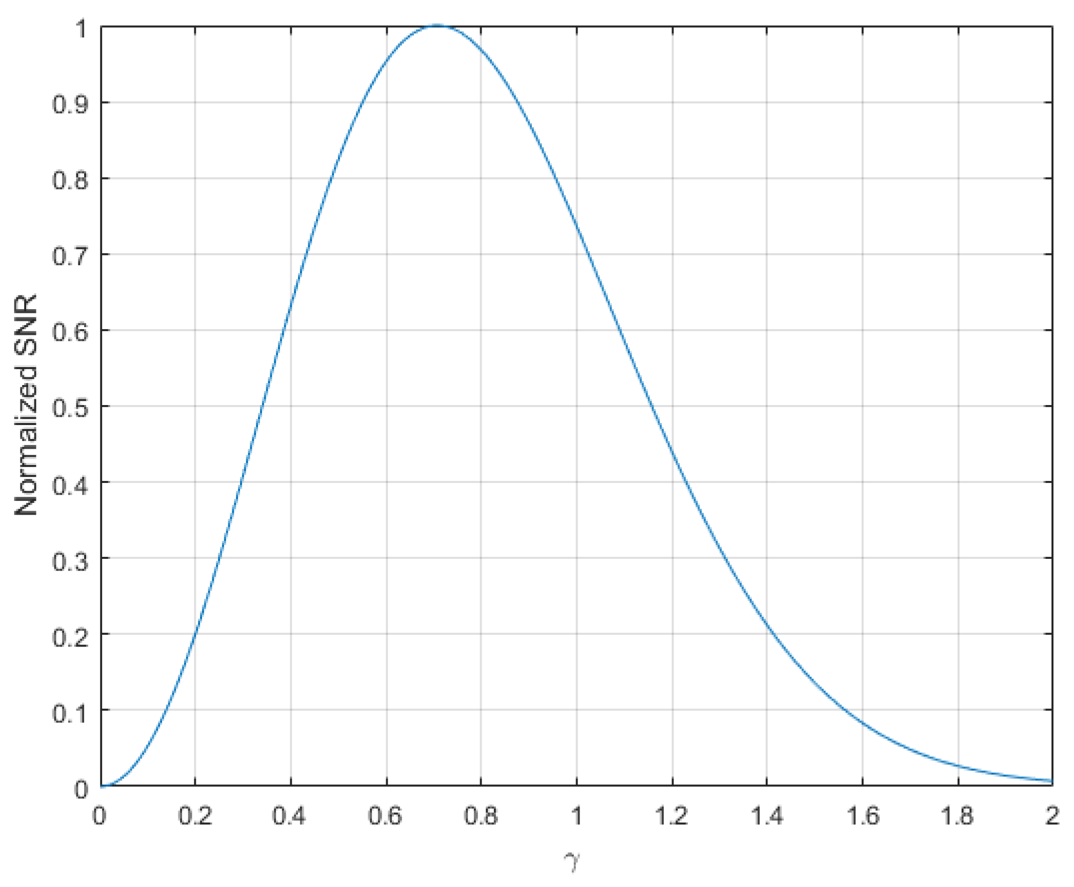
4. Angular Accuracy Estimation

The L/R channel is connected to a radiometer that measures the antenna noise temperatures:

$$\begin{array}{c}T{A}_{f1}^{\ast }=T{A}_{f1}\pm {\sigma }_o\left[K\right]\hfill \\ T{A}_{f2}^{\ast }=T{A}_{f2}\pm {\sigma }_o\hfill \end{array}$$

(33)

with uncertainty [10] ${\sigma }_o=\frac{\sqrt{2}{T}_0(F-1)}{\sqrt{B_{RF}\tau }}$, $T_o$ being the standard noise temperature, F being the receiver noise figure, and $B_{RF}$ and $\tau$ being the receiver bandwidth and integration time, respectively. The uncertainty ${\sigma }_o$ is equal to the root-mean-square (RMS) value of the radiometric sensitivity of the receiver operating in time-sharing. As the useful signal is the difference between the noise temperatures reported in Equation (26), the uncertitude of the difference is

$$\Delta T_A^{\ast }=\Delta TA\pm {\sigma }_{\Delta }$$

(34)

with

$${\sigma }_{\Delta }=\sqrt{2}{\sigma }_o=\frac{2T_0(F-1)}{\sqrt{B_{RF}\tau }}$$

(35)

When

$$M=\Delta T_T(\frac{\Delta {\vartheta }_T^2}{{\vartheta }_{3dB}^2})e^{-2\frac{\Delta {\vartheta }_T^2}{{\vartheta }_{3dB}^2}}$$

(36)

one obtains

$$\Delta T_A^{\ast }(\beta )=M{\left[4\log (2)\right]}^2\frac{\beta }{{\vartheta }_{3dB}}\pm {\sigma }_{\Delta }$$

(37)

Therefore, the estimated angle is

$${\beta }^{\ast }=\frac{{\vartheta }_{3dB}}{{\left[4\log (2)\right]}^{2}M}\Delta T_A^{\ast }(\beta )\pm \frac{{\vartheta }_{3dB}}{{\left[4\log (2)\right]}^{2}M}{\sigma }_{\Delta }$$

(38)

and defining the radiometric SNR (Signal to Noise Ratio) as

$$SNR=\frac{\Delta T_T(\frac{\Delta {\vartheta }_T^2}{{\vartheta }_{3dB}^2})e^{-2\frac{\Delta {\vartheta }_T^2}{{\vartheta }_{3dB}^2}}}{{\sigma }_{\Delta }}$$

(39)

the angular error is given by

$${\sigma }_{\beta }=\frac{1}{{\left[4\log (2)\right]}^2}\frac{{\vartheta }_{3dB}}{SNR}\cong \frac{{\vartheta }_{3dB}}{7.68}\frac{1}{SNR}$$

(40)

where

$$\Delta {\vartheta }_T^2\cong \frac{A_T}{\pi R^2}$$

(41)

We have considered the atmospheric attenuation to be negligible, and thus, Equation (39) can be rewritten as

$$SNR(R)=\Delta T_T\frac{A_T}{{\sigma }_{\Delta }\pi R^2{\vartheta }_{3dB}^2}{e}^{(-\frac{2A_T}{\pi R^2{\vartheta }_{3dB}^2})}.$$

(42)

The following being the error on the $\beta$ angle:

$${\sigma }_{\beta }=\frac{{\vartheta }_{3dB}}{7.68}\frac{\pi R^2{\vartheta }_{3dB}^2{e}^{\frac{2A_T}{\pi R^2{\vartheta }_{3dB}^2}}}{\Delta T_T{A}_T}$$

(43)

the radiometric delta signal (Equation (32)) can be normalized with respect to the “sum” signal in order to minimize the contribution due to the variation of the target radiometric contrast on the angular estimation, as described later.

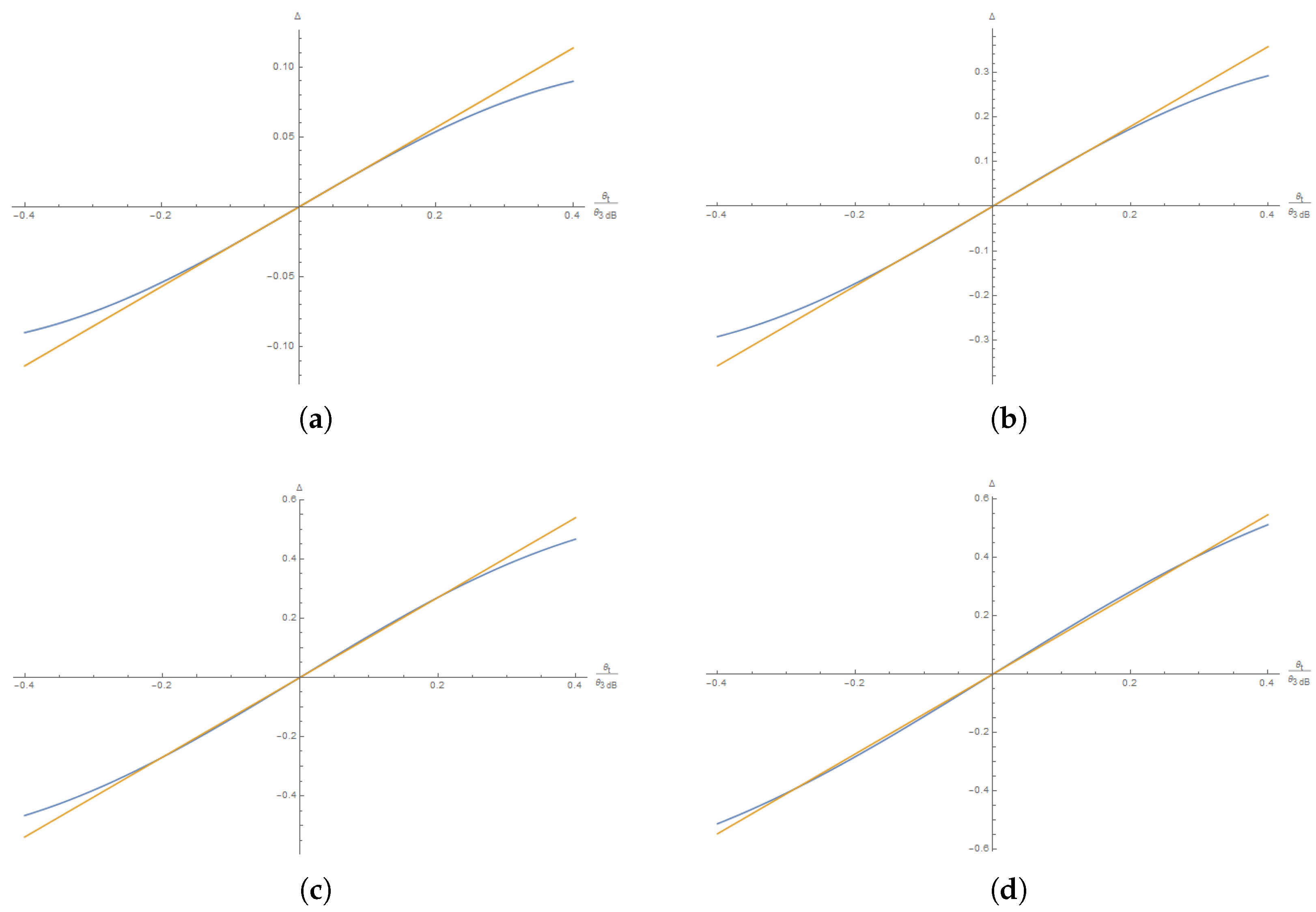
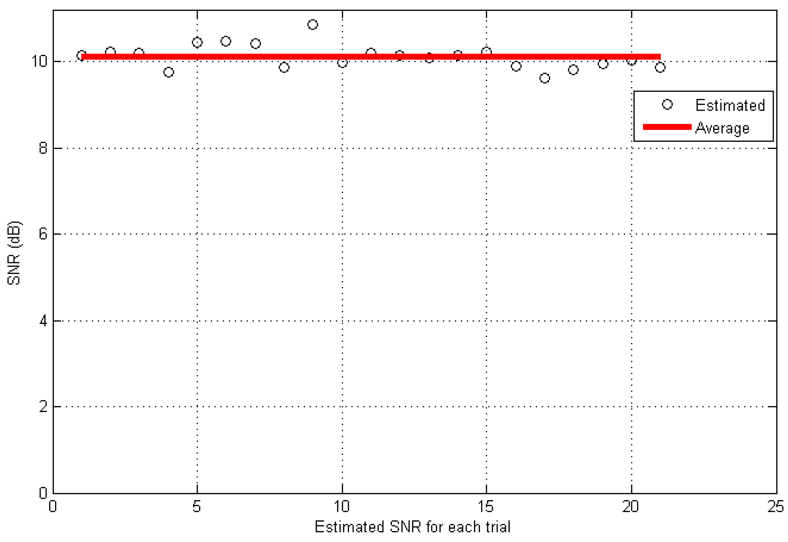
5. Estimated Results

For a sensor operating at 94 GHz using state-of-the-art millimeter-wave components, it is reasonable to assume that [11] ${\vartheta }_{3dB}=1$ (°) and ${\sigma }_{\Delta }\cong 150$ (mK). Moreover, it is reasonable to consider a target with $A_T=30$ (m²), with a radiometric contrast $\Delta T_T\cong 100$ (K). A SNR of ≥8 (dB) (P_d = 0.9 and P_fa = 10⁻⁶ respectively the detection probability and false alarm probability) ensures an angular error of ∼0.45 mrad (∼ 2/100 of degree) at a distance R∼ 2 Km, as reported in Figure 8 and Figure 9.

The target is seen by the sensor as a point, and this condition is implicit in Equation (32). It can be demonstrated that the SNR has a maximum when $\frac{\Delta {\vartheta }_T^2}{{\vartheta }_{3dB}^2}=\frac{1}{2}$. It is easily perceivable that, when the target distance is small enough to make $T{A}_{f1}\cong T{A}_{f2}$, the SNR falls rapidly to zero while the angular error diverges. This condition, however, corresponds to the final impact instants considering the high negative rate of variation of R. Looking at the behaviour of the normalized SNR expression of Equation (39) as a function of the ratio $\gamma =\frac{\Delta {\vartheta }_T}{{\vartheta }_{3dB}}$, as depicted in Figure 10, it is possible to find out a range of $\gamma$ values for which, for the same target radiometric contrast, the SNR is high enough to allow target tracking with an acceptable angular error. A SNR of ≥8 (dB) requires

$$\sqrt{\frac{-W(-2·{10}^{\frac{4}{5}}\frac{\sigma }{\Delta T_T})}{2}}\le \gamma \le \sqrt{\frac{-W(-1,-2·{10}^{\frac{4}{5}}\frac{\sigma }{\Delta T_T})}{2}}$$

(44)

where W(x) is the Lambert function, $\sigma$ is the radiometric sensitivity and $\Delta$T_T is the target radiometric contrast. With the parameters equal to those used previously, it follows that $\gamma \cong 0.098$ and $\gamma \cong 1.69$, which corresponds to

$$105\le R\le 1800(\mathrm{m})$$

(45)

6. Extension to a Pseudo-Monopulse Architecture

The exclusive use of the “difference” signal makes the sensor dependent on the variations of the radiometric target contrast. For this purpose, it is possible to think to a pseudo-monopulse architecture, for which the difference signal is normalized to the sum signal. The corresponding analysis requires better approximations of the antenna noise temperatures. The use of normalized forms with respect the 3 dB angle of $\Delta {\vartheta }_T$, ${\vartheta }_o$ and ${\vartheta }_t$ allows for the identification of suitable approximate expressions for L/R beams’ antenna noise temperatures through numerical integration and parameter fitting. For target angular positions within half of ${\vartheta }_{3dB}$ (in module), the noise temperatures have Gaussian shapes with centers coincident and with ${\vartheta }_o$ but with standard deviations dependent on the ratio $\frac{{\vartheta }_t}{{\vartheta }_{3dB}}$. Suitable expressions for the antenna noise temperatures of L/R beams are the following:

$$T_A\approx \Delta T_T(1-e^{-4\log (2)\frac{\Delta {\vartheta }_T^2}{{\vartheta }_{3dB}^2}})e^{-2\log (4)e^{-\log (4)\frac{\Delta {\vartheta }_T^2}{{\vartheta }_{3dB}^2}}{(\frac{{\vartheta }_t}{{\vartheta }_{3dB}}-\frac{{\vartheta }_o}{{\vartheta }_{3dB}})}^2}+T_s$$

(46)

$$T_B\approx \Delta T_T(1-e^{-4\log (2)\frac{\Delta {\vartheta }_T^2}{{\vartheta }_{3dB}^2}})e^{-2\log (4)e^{-\log (4)\frac{\Delta {\vartheta }_T^2}{{\vartheta }_{3dB}^2}}{(\frac{{\vartheta }_t}{{\vartheta }_{3dB}}+\frac{{\vartheta }_o}{{\vartheta }_{3dB}})}^2}+T_s$$

(47)

If the contribution due to T_s is small enough, it is possible to evaluate the ratio

$$\frac{\Delta }{\Sigma }=\frac{T_A-T_B}{T_A+T_B}$$

(48)

If the target angular coordinate is close to the antenna axis, it is possible to write

$$\frac{\Delta }{\Sigma }\cong 2\frac{2^{-2\frac{\Delta {\vartheta }_T^2}{{\vartheta }_{3dB}^2}}}{{\vartheta }_{3dB}}\log (4){\vartheta }_t$$

(49)

The ratio is independent from the radiometric contrast of the target $\Delta T_T$. The sensor works by determining separately and independently the random variables

$$X_1=T_A^{\ast }-T_B^{\ast }$$

(50)

and

$$Y_1=T_A^{\ast }+T_B^{\ast }$$

(51)

The estimation of the angular coordinate of the target is done using a new random variable:

$$Z=\frac{X_1}{Y_1}$$

For the physics of the device, the following can be demonstrated [10]:

• X₁ is a Gaussian random variable with expected value ${\mu }_1=T_A-T_B$ and variance ${\sigma }^2={\sigma }_A^2+{\sigma }_B^2$.
• Y₁ is a Gaussian random variable with expected value ${\mu }_2=T_A+T_B$ and variance ${\sigma }^2={\sigma }_A^2+{\sigma }_B^2$.

Thus, $T_A^{\ast }$ and $T_B^{\ast }$ can be assumed to be uncorrelated and with the same variance ${\sigma }^2$. The standard deviation of Z is as follows [12]:

$${\sigma }_Z\cong \left|\frac{{\mu }_1}{{\mu }_2}\right|\sigma \sqrt{(\frac{1}{{\mu }_1^2}+\frac{1}{{\mu }_2^2})}$$

(52)

However ${\mu }_1\ll {\mu }_2$, and thus

$${\sigma }_Z\cong \left|\frac{1}{{\mu }_2}\right|\sigma$$

(53)

Evaluating the sum signal around the origin:

$${\sigma }_Z\cong \left|\frac{1}{{\mu }_2}\right|\sigma \cong \frac{2^{-1+2\frac{\Delta {\vartheta }_T^2}{{\vartheta }_{3dB}^2}}}{\Delta T_T(1-e^{-4\log (2)\frac{\Delta {\vartheta }_T^2}{{\vartheta }_{3dB}^2}})}\sigma$$

(54)

and defining the sum channel SNR as

$$SN{R}_{\Sigma }=\frac{1}{\sigma }\frac{\Delta T_T(1-e^{-4\log (2)\frac{\Delta {\vartheta }_T^2}{{\vartheta }_{3dB}^2}})}{2^{-1+2\frac{\Delta {\vartheta }_T^2}{{\vartheta }_{3dB}^2}}}$$

(55)

then

$${\sigma }_Z\cong \frac{1}{SN{R}_{\Sigma }}$$

(56)

The angular position of the target is tied with the ratio $\frac{\Delta }{\Sigma }$:

$${\vartheta }_t=\frac{{\vartheta }_{3dB}}{2^{1-2\frac{\Delta {\vartheta }_T^2}{{\vartheta }_{3dB}^2}}\log (4)}\frac{\Delta }{\Sigma }$$

(57)

Thus, the RMS angular error is

$${\sigma }_{{\vartheta }_t}=\frac{1}{2\log (4)}\frac{1}{SN{R}_{\Sigma }}{e}^{2\frac{\Delta {\vartheta }_T^2}{{\vartheta }_{3dB}^2}}{\vartheta }_{3dB}$$

(58)

Defining the slope of the difference channel normalized to the maximum value as

$$K_m=2^{-2\frac{\Delta {\vartheta }_T^2}{{\vartheta }_{3dB}^2}}$$

(59)

then the angular error is

$${\sigma }_{{\vartheta }_t}\cong \frac{{\vartheta }_{3dB}}{2.77K_m}\frac{1}{SN{R}_{\Sigma }}$$

(60)

The parameter

$$\alpha =\frac{\Delta {\vartheta }_t}{{\vartheta }_{3dB}}$$

(61)

allows us to easily represent the SNR ratios on the sum and difference channels, as well as the angular error. Assuming, as done previously, a radiometric contrast of 100 (K) and a sensor sensitivity of 150 (mK), the theoretical angular error is reported in Figure 11.

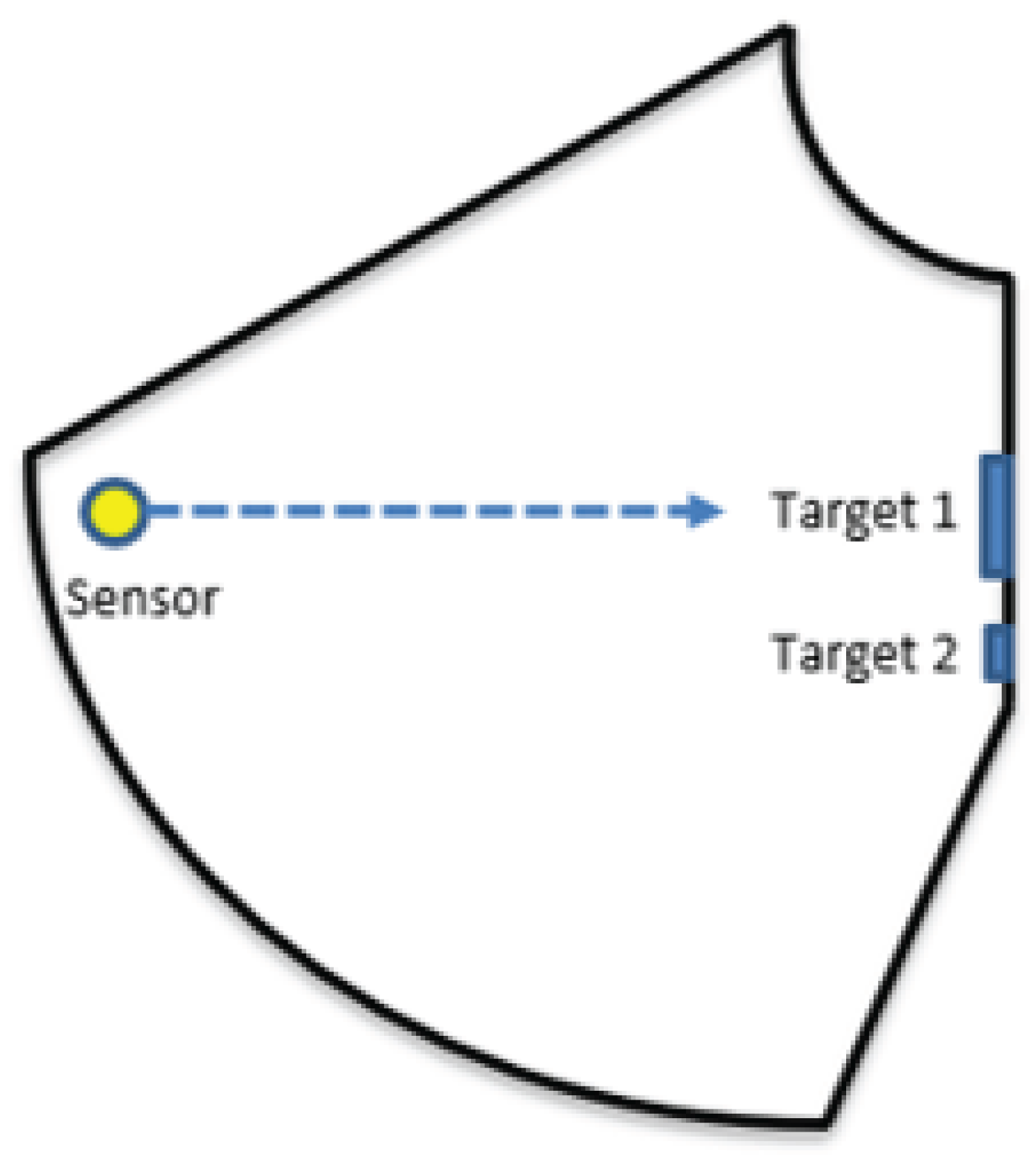
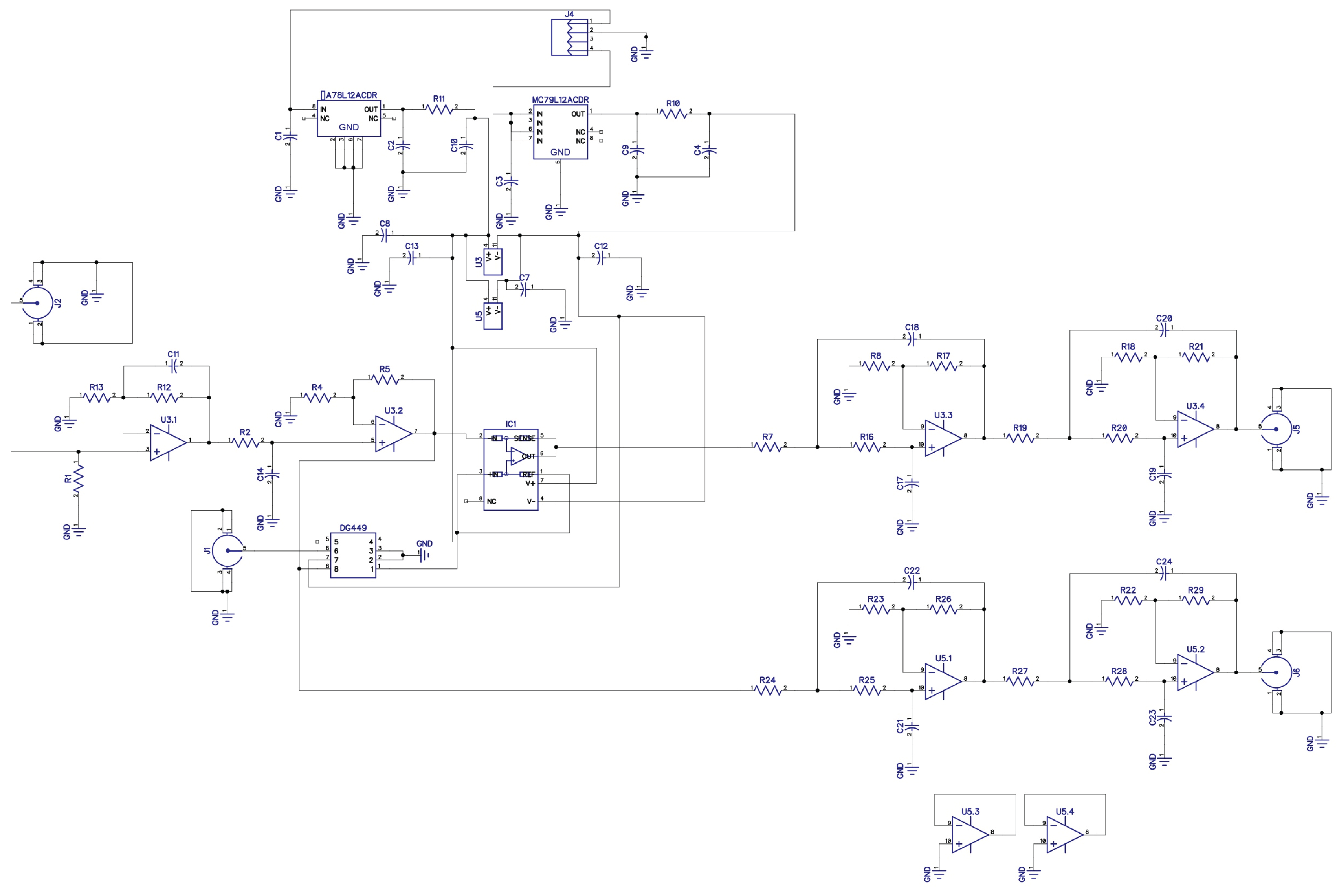
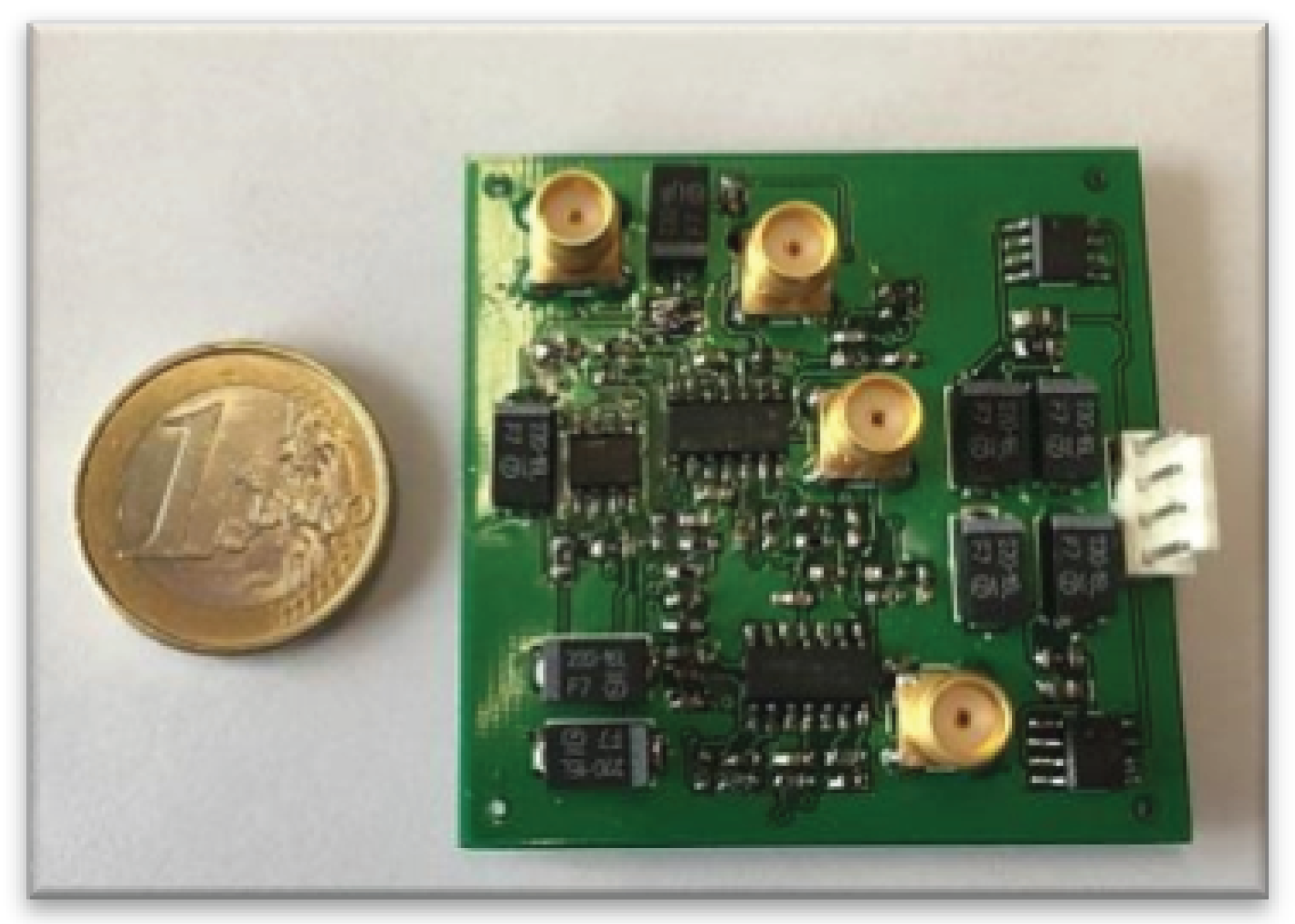
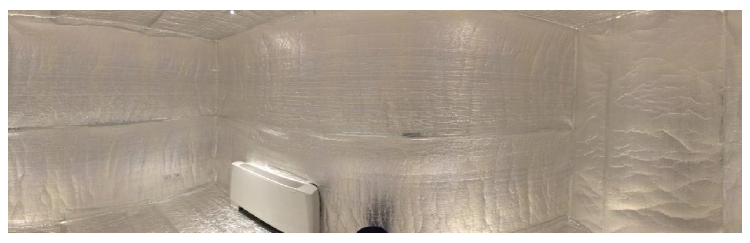
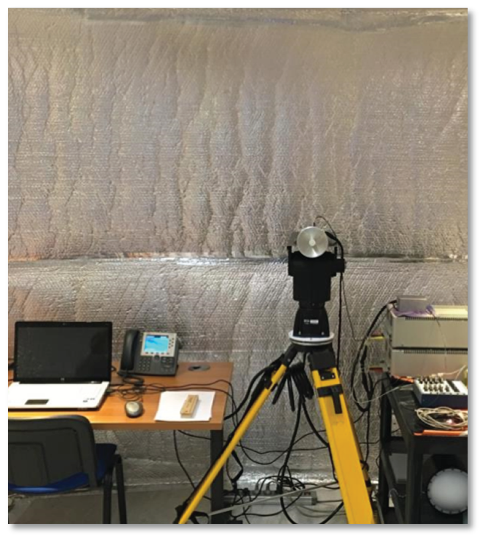
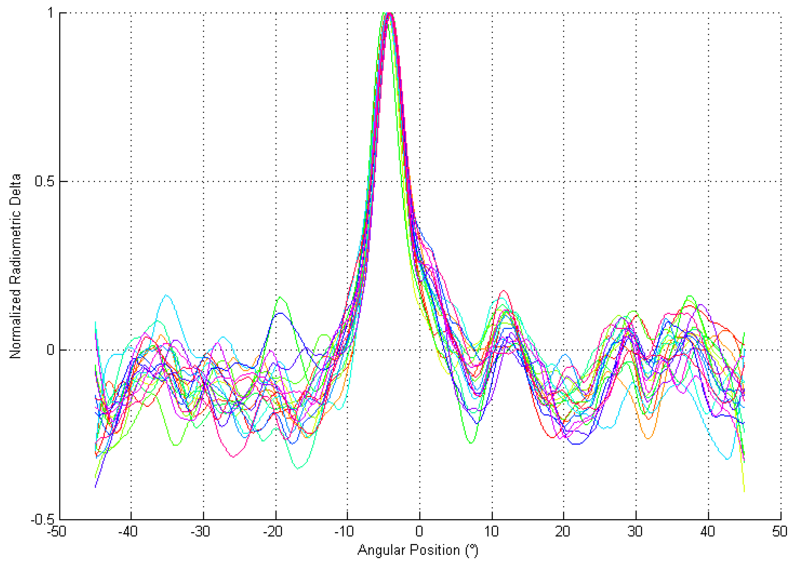
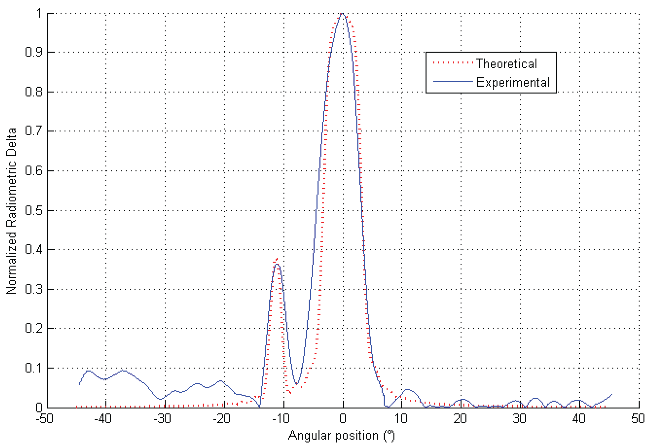
7. Experimental Results

To validate the theory, a near-zero emissivity chamber was dedicated to the test of a custom W-band sensor. The laboratory walls were completely covered by a 30 skin-depths-thick aluminium sheet in order to obtain a “cold” room or a low emissivity environment, as visible in Figure 12.

In Figure 13, a simplified layout of the area with crooked walls in order to minimize successive reflections inside the volume is reported. The sensor is located on the left, and two passive targets (Eccosorb panels), “Target 1” and “Target 2”, with dimensions of 30 × 30 cm and 15 × 15 cm respectively are on the right. The space between targets and the “Target 2” dimensions were selected in order to operate at the Rayleigh limit at a distance of ≈4 (m) from the seeker’s antenna.

Experimental trials were conducted using a custom W-band sensor mounted over a Pan-Tilt Unit-D100-EX screwed over a tripod, as depicted in Figure 14, in order to control the orientation of the sensor in near real-time with high accuracy, instead of moving the targets. Laboratory tests were conducted only on the horizontal plane to minimize time and costs, while mechanical alignments and range measurements were carried out using a laser range finder.

A custom synchronous demodulator was designed (Figure 15) and realized (Figure 16) in order to integrate and conveniently amplify the signal acquired by a National Instruments DAQ 6356.

A preliminary test was performed in order to estimate the available SNR inside the cold room and to obtain a rough target position angular accuracy. For this purpose, a human target with a known emissivity $ϵ\approx$ of 0.8 was located between “Target 1” and “Target 2”, temporarily covered by a metal sheet, and the system was programmed to explore a 90° wide angular sector 25 times. The target was always detected as reported in Figure 17, allowing a rough position estimation of $\theta$ ≈ −4.2 ± 0.2° with a SNR of about 10 dB, as reported in Figure 18.

Then the human target was removed and the passive targets uncovered. Thus, a 90° wide angular sector was scanned with an angular speed of 45°/s in order to search and identify the targets reported in Figure 19, obtaining two distinct radiometric pulses in considerable agreement with an integral model developed in Matlab and reported in Figure 20 in a normalized form.

Once the potential targets were acquired, the computer selected the largest (“Target 1” hit by the laser spot in Figure 19), commanding the positioner to move to the corresponding position. A small angular sector scan was performed around this position, in order to extract the “S” function reported in Figure 21. The authors did their best to minimize systematic errors using an antenna system that was characterized in an anechoic chamber in order to be confident that the principal main requirements were respected by the manufacturer. Moreover, the differential nature of the synchronous demodulator allowed us to minimize residual DC offset, while the use of a laser rangefinder allowed us to minimize range calculation errors or residual angular displacement errors. The main error source was indeed the positioner, as the device was used either to command or also to read the true sensor angular position using an internal resolver. Considering, as stated previously, the only main random sources of errors being independent and Gaussian in nature, the true angular accuracy was estimated as a RMS value. The difference between the estimated theoretical angular accuracy ${\sigma }_{\theta }\approx 0.015$ (°) and the experimental, ${\sigma }_{\theta }\approx 0.025$ (°), appeared to be very good.

8. Conclusions

Closed formulas for evaluating the angular tracking error of a four-quadrant, double-channel millimetre-wave radiometric seeker sensor using a fast electronic sequential-lobing technique have been derived. Suitable closed formulas have been derived for a difference channel architecture and for a more accurate pseudo-monopulse architecture. The theory has been validated through experimental trials performed in a dedicated low-emissivity room using a custom W-band sensor. It has been demonstrated that a passive millimeter-wave sensor can provide guidance information (like a passive infrared sensor), and the results indicate that the angular error is proportional to $SN{R}^{-1}$ and not to $SN{R}^{-\frac{1}{2}}$, as for classical radars [13,14,15]. Moreover, the pseudo-monopulse architecture needs only two independent receivers, but these are not required to be matched. During the homing phase, when the distance to the target is relatively small, the technique can provide very accurate target tracking data.

References

1. Alimenti, F.; Bonafoni, S.; Leone, S.; Tasselli, G.; Basili, P.; Roselli, L.; Solbach, K. A Low-Cost Microwave Radiometer for the Detection of Fire in Forest Environments. IEEE Trans. Geosci. Remote Sens. 2008, 46, 2632–2643. [Google Scholar] [CrossRef]
2. Alimenti, F.; Roselli, L.; Bonafoni, S. Microwave Radiometers for Fire Detection in Trains: Theory and Feasibility Study . Sensors 2016, 16. [Google Scholar] [CrossRef] [PubMed]
3. Jacobs, E.L.; Furxhi, O. Target identification and navigation performance modeling of a passive millimeter wave imager. Appl. Opt. 2010, 49, E94–E105. [Google Scholar] [CrossRef] [PubMed]
4. Nanzer, J. Microwave and Millimeter-Wave Remote Sensing for Security Applications; Artech House: Norwood, MA, USA, 2012. [Google Scholar]
5. Kapilevich, B.; Litvak, B.; Shulzinger, A.; Einat, M. Portable Passive Millimeter-Wave Sensor for Detecting Concealed Weapons and Explosives Hidden on a Human Body. IEEE Sens. J. 2013, 13, 4224–4228. [Google Scholar] [CrossRef]
6. James, D. Radar Homing Guidance for Tactical Missiles; Mac Millan Education Ltd.: London, UK, 1986. [Google Scholar]
7. Patton, R.B., Jr.; Wilson, C.L. The VARR Method, a Technique for Determining the Effective Power Patterns of Millimeter-Wave Radiometric Antennas; BRL Report No. 1322; Defense Technical Information Center: Fort Belvoir, VA, USA, 1966. [Google Scholar]
8. Balanis, C.A. Antenna Theory: Analysis and Design, 2nd ed.; John Wiley and Sons Inc.: Hoboken, NJ, USA, 1997. [Google Scholar]
9. Otoshi, T.Y. Noise Temperature Theory and Applications for Deep Space Communications Antenna Systems; Artech House: Norwood, MA, USA, 2008. [Google Scholar]
10. Racette, P.E.; Lang, R.H. Radiometer design analysis based upon measurement uncertainty. Radio Sci. 2005, 4, RS5004. [Google Scholar] [CrossRef]
11. Skou, N. Microwave Radiometer Systems: Design and Analysis, 2nd ed.; Artech House: Norwood, MA, USA, 2006. [Google Scholar]
12. Stuart, A.; Ord, K. Kendall’s Advanced Theory of Statistics, 6th ed.; Arnold: London, UK, 1998; Volume 1. [Google Scholar]
13. Levanon, N. Radar Principles; John Wiley and Sons Inc.: New York, NY, USA, 1988. [Google Scholar]
14. Barton, D.K.; Sherman, S.M. Monopulse Radar Theory and Practice, 2nd ed.; Artech House: Norwood, MA, USA, 2011. [Google Scholar]
15. Klein, L.A. Millimeter-Wave and Infrared Multisensor Design and Signal Processing; Artech House: Norwood, MA, USA, 1997. [Google Scholar]
Figure 1. Diamond-shaped Cassegrain feed.
Aerospace 05 00011 g001
Figure 2. Radiometric seeker sensor 3 dB contours.
Aerospace 05 00011 g002
Figure 3. Simplified system-level schematic of a fast sequential-lobing radiometric seeker sensor.
Aerospace 05 00011 g003
Figure 4. Squinted Gaussian power patterns.
Aerospace 05 00011 g004
Figure 5. Target and left/right (L/R) beams’ geometry.
Aerospace 05 00011 g005
Figure 6. Corrective factor to be applied to the approximated formula.
Aerospace 05 00011 g006
Figure 7. Radiometric deltas extracted numerically (blue) and using the closed approximated formula (yellow) for different values of parameter x.
Aerospace 05 00011 g007
Figure 8. SNR as a function of the distance from the target.
Aerospace 05 00011 g008
Figure 9. Angular error as a function of the distance from the target.
Aerospace 05 00011 g009
Figure 10. Behaviour of the normalized SNR as a function of γ (Equation (39)).
Aerospace 05 00011 g010
Figure 11. Angular error as a function of the ratio α .
Aerospace 05 00011 g011
Figure 12. “Cold” laboratory chamber.
Aerospace 05 00011 g012
Figure 13. Laboratory layout.
Aerospace 05 00011 g013
Figure 14. W-band sensor mounted on pan and tilt unit.
Aerospace 05 00011 g014
Figure 15. Synchronous demodulator scheme.
Aerospace 05 00011 g015
Figure 16. Actual synchronous demodulator.
Aerospace 05 00011 g016
Figure 17. Human target radiometric pulses during repeated search phase (superimposed traces).
Aerospace 05 00011 g017
Figure 18. Estimated available SNR.
Aerospace 05 00011 g018
Figure 19. Passive “Target 1” and “Target 2”.
Aerospace 05 00011 g019
Figure 20. Radiometric pulses after search of two passive targets.
Aerospace 05 00011 g020
Figure 21. “S” function derived experimentally.
Aerospace 05 00011 g021