Predicting Non-Linear Flow Phenomena through Different Characteristics-Based Schemes


Centre for Computational Engineering Sciences, Cranfield University, Cranfield, Bedfordshire MK43 0AL, UK
*
Author to whom correspondence should be addressed.
Aerospace 2018, 5(1), 22; https://doi.org/10.3390/aerospace5010022
Submission received: 18 November 2017
/
Revised: 7 January 2018
/
Accepted: 18 February 2018
/
Published: 24 February 2018
(This article belongs to the Special Issue Computational Aerodynamic Modeling of Aerospace Vehicles)
Abstract
:The present work investigates the bifurcation properties of the Navier–Stokes equations using characteristics-based schemes and Riemann solvers to test their suitability to predict non-linear flow phenomena encountered in aerospace applications. We make use of a single- and multi-directional characteristics-based scheme and Rusanov’s Riemann solver to treat the convective term through a Godunov-type method. We use the Artificial Compressibility (AC) method and a unified Fractional-Step, Artificial Compressibility with Pressure-Projection (FSAC-PP) method for all considered schemes in a channel with a sudden expansion which provides highly non-linear flow features at low Reynolds numbers that produces a non-symmetrical flow field. Using the AC method, our results show that the multi-directional characteristics-based scheme is capable of predicting these phenomena while the single-directional counterpart does not predict the correct flow field. Both schemes and also Riemann solver approaches produce accurate results when the FSAC-PP method is used, showing that the incompressible method plays a dominant role in determining the behaviour of the flow. This also means that it is not just the numerical interpolation scheme which is responsible for the overall accuracy. Furthermore, we show that the FSAC-PP method provides faster convergence and higher level of accuracy, making it a prime candidate for aerospace applications.
1. Introduction
Despite the advances made in the field of computational fluid dynamics over the past decades, predicting flow patterns around aerodynamic shapes remains a challenge for aerospace applications. The flow around a wing can have a transonic behaviour which, at high angles of attack, may be supplemented by flow separation, strong crossflow gradients as well as a hysteresis in the lift slope [1,2]. Traub [3] highlighted further that at low Reynolds number flows, laminar separation bubbles exist which have an inherently unsteady behaviour. These separation bubbles may reattach to the wing or transition into a fully turbulent flow, depending on the pressure gradient. Panaras [4] reviewed recent published studies on Reynolds-averaged Navier–Stokes (RANS) and large-eddy simulation (LES) results and pointed out that the turbulent kinetic energy in regions of reversed flow is low and can be considered to be almost laminar. Thus, it is important to capture the transition between laminar and turbulent flows as flow separation and reattachment ultimately have a strong influence on predicting the lift slope, stall angle and hysteresis. Furthermore, since RANS models are commonly based on the linear Boussinesq assumption, results may provide only a moderate accuracy while models based on non-linear theories may be more efficient in predicting non-isotropic flow behaviour.
From the considerations given above, it is important to realize that the non-linear term in the Navier–Stokes equations is the most sensitive part and an accurate numerical description is mandatory to capture those flow features. The literature on numerical schemes is vast and this article does not intend to give a comprehensive overview—interested readers are referred to reference [5,6]—however a brief overview is given. Initially the second-order central scheme was used and later augmented by artificial dissipation. This was necessary to account for the lost dissipation on the small scales due to an under-resolved computational grid, essentially mimicking the same approach RANS turbulence model take in order to provide turbulent, or physical, dissipation. The central scheme lacks transportiveness and so is not suitable to predict flows containing discontinuities. A range of high-resolution schemes were developed to address this issue, of which the monotonic upwind scheme for conservation laws (MUSCL), total variation diminishing (TVD), essential non-oscillatory (ENO) and weighted essential non-oscillatory (WENO) schemes are the most widely used schemes nowadays. These schemes all have the same goal; to capture the correct behaviour of the non-linear term. However, their closure is based on numerical considerations. In order to enhance these scheme and to provide highly-accurate physical values for the time integration procedure, two possible routes are available. The first one is commonly employed in the compressible community where an approximate Riemann solver (RS) is used. In-fact, by including the local Riemann problem, the values obtained through the numerical scheme are modified based on the local eigenstructure of the system of equations, thus presenting a hybrid approach to couple numerical and physical fluxes. The second approach is to take a characteristics-based (CB) scheme which shares many similarities of the local Riemann problem, although being rather different in the details. Here, the characteristics of the flow are found at each computational node where the primitive variables are updated along the compatibility equations, which are unique to each node. The CB scheme found widespread use in the 1960s and onwards for the calculation of compressible flows [7].
With the introduction of the Artificial Compressibility (AC) method of Chorin [8], which was the first hyperbolic method available in the framework on incompressible flows, it became possible to apply both the local Riemann problem as well as CB schemes to incompressible flows. Drikakis et al. [9] were among the first to introduce the CB scheme in conjunction with the AC method in the finite volume method, which was followed by a development in the finite element framework by Zienkiewicz and Codina [10] and Zienkiewicz et al. [11]. The CB scheme of Drikakis [9] was developed for one-dimensional flows but can be extended to higher dimensions by applying the same equations to any coordinate direction in space. Thus, the approach is termed the single-directional characteristics-based, or SCB, scheme. The scheme was later revised by Neofytou [12] and tested by Su et al. [13], concluding that, although the revised scheme being more mathematical rigorous, there was little difference in the results using the original and revised SCB scheme.
A vastly different approach was taken by Razavi et al. [14] who proposed to use a multi-directional characteristics-based, or MCB, scheme. It was extended to handle curve-linear coordinate systems [15] as well as unstructured grids [16]. Improved boundary conditions in combination with the MCB scheme was proposed by Hashemi and Zamzamian [17] for the far-field and Zamzamian and Hashemi [18] for solid boundary conditions. Fathollahi and Zamzamian [19] investigated the influence of the number of compatibility equations used at each node. They showed that increasing the number of compatibility equation did not affect the accuracy of the solution while increasing the convergence rate. The scheme has been tested for heat transfer and turbulent flows by Razavi and Adibi [20] and Razavi and Hanifi [21], respectively. In the MCB scheme, instead of tracking characteristic lines through each computational node as done in the SCB scheme, characteristic surfaces are multiplied into the governing equations and their solution is found by means of the system’s eigenvalues and geometrical considerations. This creates a characteristic cone along which the compatibility equations are emanating. This allows the scheme to capture any anisotropic properties of the flow and therefore lends itself to capture non-linear flow features.
In the present work, our aim is to show the applicability of the MCB scheme to predict non-linear flow behaviours at low reynolds numbers. As a comparison, we also employ the SCB scheme and apply Rusanov’s RS which provides a hybrid multi-directional, Godunov-type treatment for the non-linear term of the Navier–Stokes equations. We apply the scheme to a channel with a sudden expansion. This geometry was found to be particularly suitable to predict the onset of bifurcation and subsequently the reattachment point of the flow. Both phenomena are underlying features that are important to calculate turbulent flows and thus highly relevant to the discussion in the context of aerospace applications.
We use the AC method in order to apply the CB scheme and RS, which require a hyperbolic system of equations. Furthermore, we also employ a recent method developed by Könözsy [22], later introduced by Könözsy and Drikakis [23], which unifies Chorin’s AC method with Chorin’s and Temam’s Fractional-Step, Pressure projection (FS-PP) method [24,25] which is termed the Fractional-Step, Artificial Compressibility with Pressure-Projection, or FSAC-PP method (see Section 2.2). It has been tested for classical benchmark cases for incompressible flows [22], multi-species and variable density flows in micro-channels [26], trapping and positioning of cryogenic propellants [27], forced separated flows over a backward facing step [28] and the vortex pairing problem [29]. The FSAC-PP method was originally introduced using the SCB scheme and extended by Teschner et al. [30] to the MCB scheme. Smith et al. [31] removed the CB approach and used different Riemann solvers instead to obtain the inviscid fluxes. The FSAC-PP has shown to have superior convergence properties over the AC and FS-PP method, especially in low Reynolds number flows, while showing a similar level of accuracy.
The remaining structure of this article is as follows. In Section 2, we give numerical details on the AC and FSAC-PP method. Section 3 summarises the SCB and MCB scheme used in this study while the computational setup is presented in Section 4. We present the results for the sudden expansion geometry in Section 5 and highlight final remarks in Section 6.
2. Methodology
In this section, we briefly review the concepts of the AC and FSAC-PP method, which are employed throughout this study. Details can be found in [8] about the AC method and in [22,23] about the FSAC-PP approach.
2.1. The Artificial Compressibility Method
The absence of a thermodynamic functional relationship between the pressure and density has led to the notion of an Artificial Compressibility approach. Here, the density is replaced by the pressure in the time derivative of the continuity equation. Since it could be difficult to give a clear relationship between the two state variables, a numerical constant is introduced, , which is a user-defined convergence parameter [8]. Thus, the continuity equation loses any physical meaning, however, it provides a mechanism to predict the pressure in the momentum equation. Once a steady state is obtained, the time derivative vanishes to zero and so a divergence-free velocity field is obtained. The governing equations with the extensions of the AC method thus become
where and are the density and viscosity, respectively. The equations are iterated in pseudo-time due to the non-physical time derivative of pressure. In order to advance the system of Equations (1) and (2) in real time, a dual-time stepping procedure needs to be employed for which a real time derivative is added to the momentum equation. The time-step has to satisfy the following condition as
2.2. The Unified Fractional-Step, Artificial Compressibility and Pressure Projection Method
The FSAC-PP method unifies both the AC and FS-PP method into a single framework. In the first Fractional-Step, the continuity equation of the AC method is used along with the momentum equation of the FS-PP method, in which the pressure gradient is dropped. The governing equations of the numerical method can be written in a semi-discretised form by
From Equations (4) and (5), we obtain an intermediate velocity field denoted by which is used in the second Fractional-Step of the numerical procedure to recover the pressure field as
The Helmholtz-Hodge decomposition requires the velocity field at time level to become divergence-free. Thus, by taking the divergence of Equation (6), the following Poisson equation for the pressure is obtained by
With an updated pressure value, we can recover the velocity at the next time level from Equation (6) as
Equations (5)–(8) are consistent with the FS-PP method of Chorin [24] and Temam [25] while Equation (4) provides an initial pressure field for the Poisson equation through the perturbed continuity equation of the AC method. Thus, the hyperbolic and elliptic features of the AC and FS-PP method are coupled through the Fractional-Step procedure which allows for a characteristics-based treatment of the convective fluxes while the pressure is stabilised through the elliptic Poisson equation.
3. Characteristic-Based Schemes for Incompressible Flows
While the FSAC-PP method was originally introduced using the SCB scheme [9], Teschner et al. [30] showed the extension to a multi-directional characteristics-based (MCB) scheme, which is based on the derivation given by Razavi et al. [14] for the AC method.
3.1. A Single-Directional Closure
The SCB scheme splits the governing equations into one-dimensional equations and assumes that the SCB scheme is equally applicable for any direction. The primitive variables are recovered in the context of the hyperbolic-type AC method as
where
The values of and are set to , when considering the x-direction and , for the y-direction, respectively. The eigenvalues are found as
The primitive variables with indices are found through Godunov’s RS
where the intercell flux values and are found through a third-order interpolation procedure, see Section 4. In the FSAC-PP method, the characteristic pressure is set to zero as it is dropped in the momentum equation. From Equations (9) and (10) it can be seen, however, that the pressure provided by the continuity equation enters the characteristic velocity field which enforces a stronger coupling between velocity and pressure. More details on the SCB scheme can be found in [9,22,23].
3.2. A Multi-Directional Closure
In contrast to the SCB scheme, the multi-directional approach applies a characteristic surface to the governing equations. For a two-dimensional flow, the governing equations of the AC method are
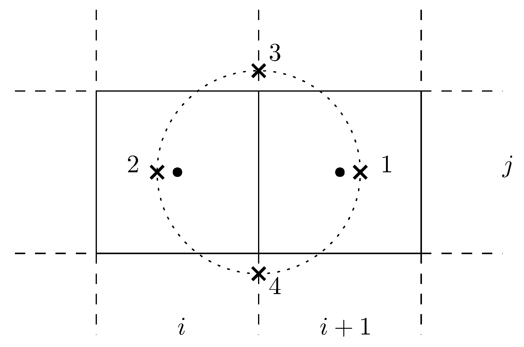
The determinant of the coefficient matrix corresponding to Equations (22)–(24) yields to solution in the form of and , where is the component of the unit normal vector and use has been made of the fact that the normal direction corresponds to the derivative of the characteristic surface in the form of . In-fact, it can be shown that corresponds to two independent characteristic surfaces [7,32,33,34] which are called the stream- () and wave- () surface in accordance with the literature on the compressible MCB scheme. Thus, inserting into Equations (23) and (24) yields two sets of compatibility equations along with Equation (22). Rusanov [7] showed that a mix of compatibility equations on and are necessarily needed to obtain the characteristic values on the cell interfaces. For the incompressible version of the MCB scheme, however, it is sufficient to only use the compatibility equations corresponding to . This can be verified by computing the rank of the coefficient matrix of Equations (22)–(24) for which will result in a non-rank deficient matrix. Thus, three compatibility equations are found over four wave directions as
The characteristic pressure is an average over all four wave directions and indicates that the velocity components, which are aligned with the wave directions, are to be used. The normal vector is
where indices correspond to the intersection of the characteristic surfaces with the time level , which is illustrated in Figure 1, and the primitive variables at those locations (wave directions) are found through interpolation. Razavi et al. [14] introduced two versions of the MCB scheme, a first- and second-order scheme, where primitive variables at are set to the reconstructed intercell variables at for the first-order scheme and are interpolated along the characteristic surfaces in the second-order scheme. Since the SCB scheme classifies as a first-order CB scheme under this definition, the first-order MCB scheme is used in the remaining investigation to compare both methods.
The SCB scheme was introduced using Godunov’s RS, Equation (18), which provided the transportiveness property of the SCB scheme. The MCB scheme, as introduced by Razavi et al. [14], did not feature any RS treatment. Thus, in order to ensure the transportiveness of the MCB scheme, a numerical interpolation scheme needs to be selected which provides this property. Alternatively, the MCB scheme can be supplemented with a RS to remove the necessity to provide transportiveness through the numerical interpolation scheme and make it a property of the MCB scheme itself. Another benefit of RS-based approaches is that different RS provide different level of numerical dissipation which may become important at high Reynolds number flows. This combination allows to use a relative cheap but high-order interpolation scheme for increased accuracy at reduced computational cost, where we make the properties traditionally linked to the numerical scheme now a property of the CB framework. Furthermore, the inclusion of the RS promotes a multi-directional Godunov-type characteristic framework for incompressible flows which has so far only been tested and introduced by Teschner et al. [30] for a simple channel geometry. Therefore, we make use of Rusanov’s approximate RS [35] in the form of
where is the inviscid flux at the cell interface from which the primitive variables are found directly through flux differentiation. We follow the approach of Davis [36] to obtain the signal velocity as
with
Using this closure, we have extended the MCB scheme into the Godunov framework and will demonstrate that even a simple approximate RS has favourable influence on the accuracy of the overall procedure.
4. Computational Setup and Numerical Schemes
The intercell values of the inviscid fluxes are obtained through a third-order interpolation polynomial as
The viscous fluxes, on the other hand, use a second-order reconstruction scheme which, for Cartesian coordinates, defaults to a finite difference discretization in the form of
The time integration is carried out by a third-order Runge–Kutta TVD scheme in which each stage is updated by the preceding one as
where
Here, we set for the AC method and for the FSAC-PP method. The numerical convergence parameter is set to , the CFL number for the explicit Runge–Kutta integration scheme is kept at while the SOR algorithm applied to the Poisson solver, Equation (7), uses an under-relaxation factor of with a total of ten Poisson iteration per time-step. Könözsy [22] found that the Poisson equation can be over-relaxed to gain further computational speed-up and suggested to use instead. Unlike the FS-PP method, in which the Poisson solver is the most computational expensive part to obtain a correct pressure field, the FSAC-PP method benefits from an initial prediction of the pressure field through the continuity equation of the AC method which substantially reduces the number of iteration needed for the Poisson equation. It was found that of the order of ten iterations is sufficient to speed up the convergence rate while keeping the same order of accuracy as obtained with the FS-PP method. The residuals are calculated based on
where is normalised based on the residual at the first iteration and compared against the convergence criterion of to ensure that the residuals have reduced by 12 orders of magnitude based on the divergence free constrain.
5. Results and Discussion
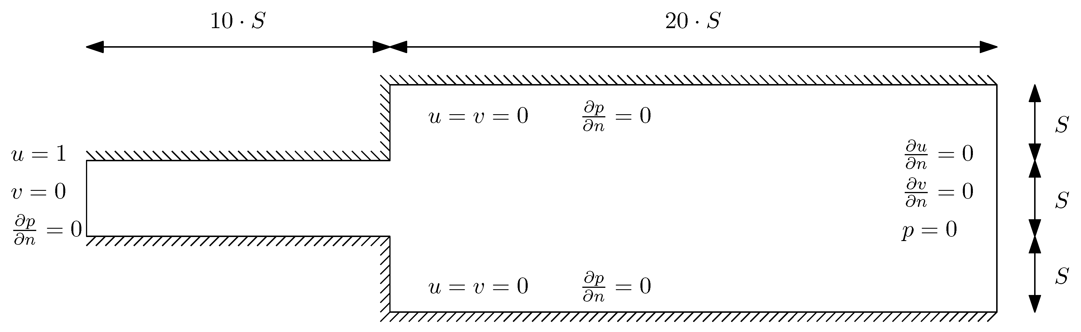
To investigate the performance of the MCB scheme using the Rusanov RS against the classical, SCB scheme, we simulate the flow inside a suddenly expanding channel with an expansion ratio of 3:1, see Figure 2. We have performed a grid convergence study and calculated the grid convergence index (GCI) based on the reattachment length according to Roache [37]. Due to the Cartesian nature of the solver, the mesh cannot be locally refined, especially near walls where a good resolution is required. This, however, creates a challenging test case for both the AC and FSAC-PP method as strong velocity gradients are present close to the wall which also amplifies any differences between the two methods. Table 1 shows the results obtained for the grid dependency study where we give the reattachment length at the upper and lower wall, as well as its corresponding GCI value and the time and iteration it took to compute the results. The Cartesian mesh elements were divided by a factor of two for subsequent mesh levels, ensuring a refinement ratio of four in all cases. We also provide the expected value based on the Richardson extrapolation which can also be found in [37]. At a Reynolds number of Re = 30, for which the GCI study has been carried out, the expected reattachment length as given by Oliveira [38] is . Looking at the results, we can see that the FSAC-PP method converges towards that results for the finest level, while the AC method fails to predict the results correctly. The FSAC-PP method also shows a lower level of GCI which is of the order of 10% while the AC method produces GCI values which are close to double of that result. In terms of relative change, the reattachment length changes less than 5% from the medium to the finest mesh level for both AC and FSAC-PP method. Although the AC method overpredicts the reattachment, in this case using no CB scheme and no RS, we will see later that the results are slightly better with other schemes. Hence, focusing on the FSAC-PP method, it would be desired to use the finest mesh level for all subsequent simulations. The computational time, however, becomes prohibitive in the case of the AC method if the finest mesh level was to be used, where a single simulation would last for more than 32 h which would cause excessive simulation times as several simulations at different Reynolds numbers are required. Furthermore, for very low Reynolds numbers, the AC method requires even more computational time [23,27]. Thus, we chose the medium mesh with 22,400 elements as the next closest mesh for which results in a reasonable amount of time can be obtained.
To ensure that the convergence criterion of is sufficient, we furthermore carried out a convergence study where we have checked the influence of the convergence parameter from to for Equation (40). To judge convergence, we check by how much the reattachment length changes on the upper and lower wall. The results are summarised in Table 2. We can see that the chosen convergence threshold at is a sufficient indicator for convergence. The results for the FSAC-PP method do not change from while the results for the AC method do only differ for the fourth significant figure. Thus, we haven chosen as a convergence threshold for all subsequent simulations.
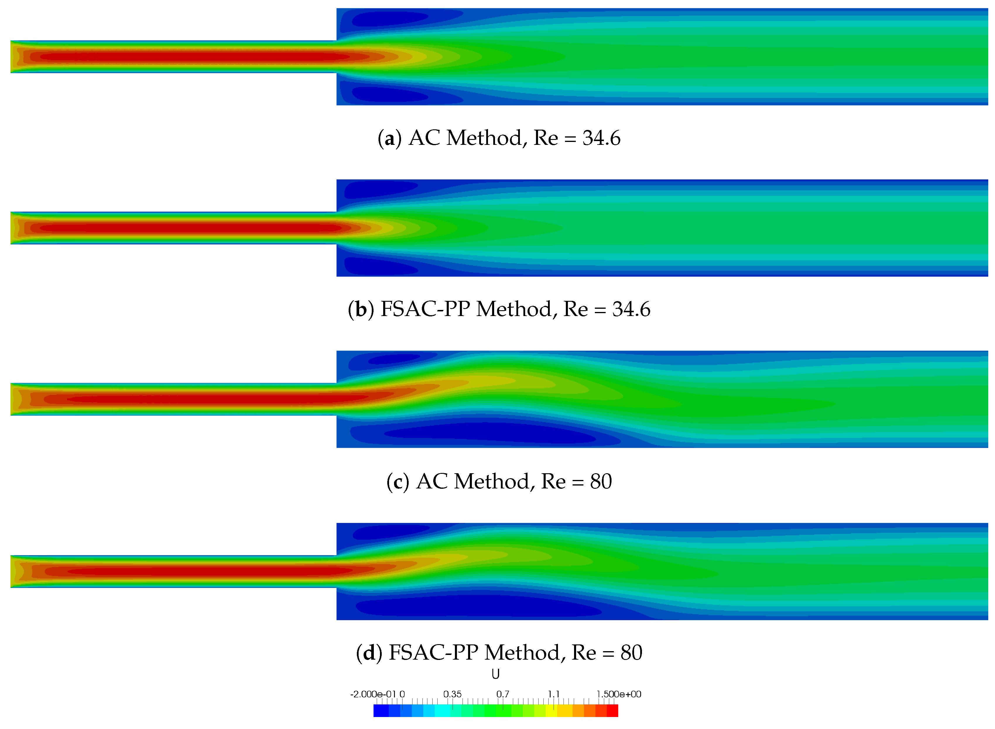
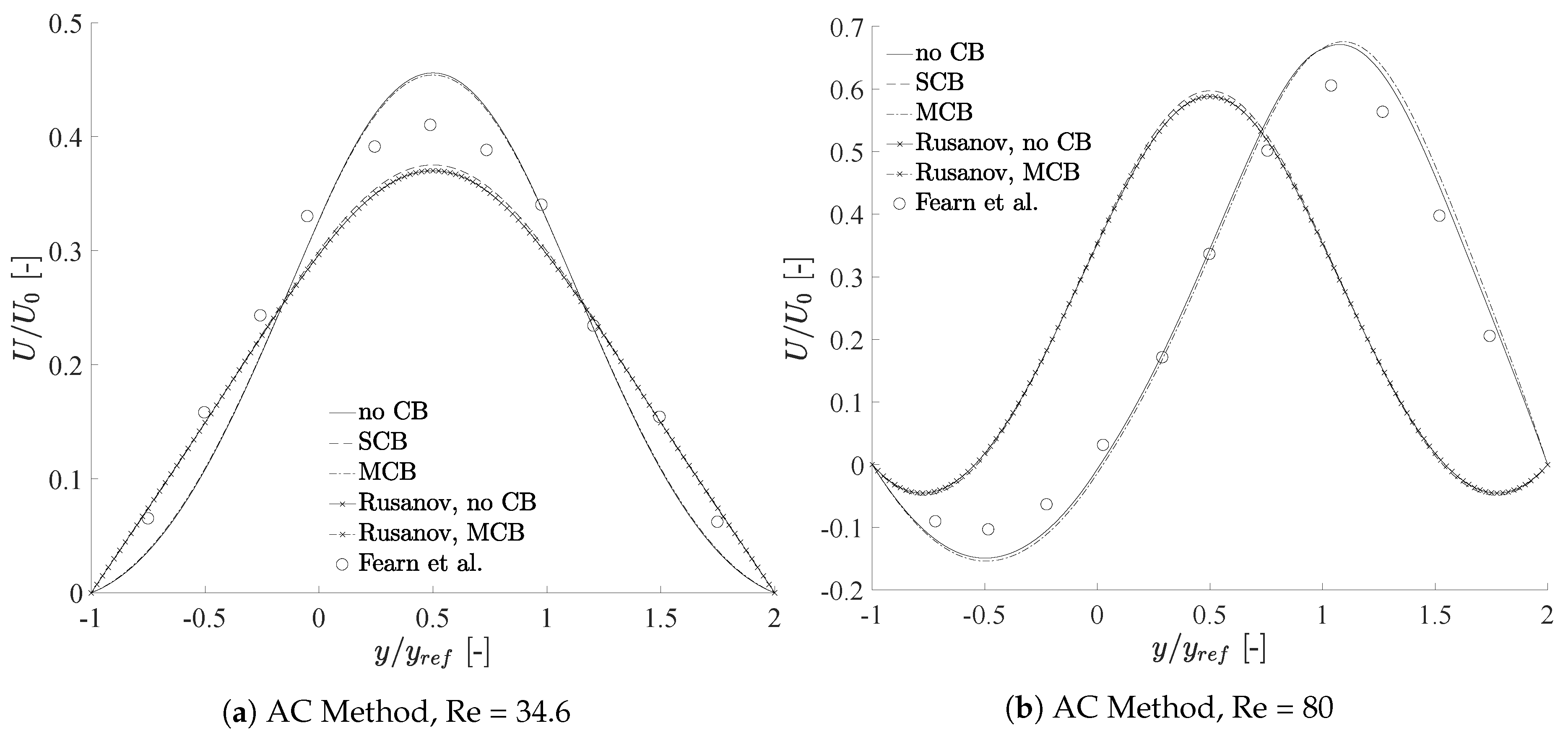
Figure 3 shows contours of the u-velocity component while Figure 4 presents the velocity profile at , where S indicates the step height, see Figure 2. We show results here obtained with the AC and FSAC-PP method for two Reynolds number. The first Reynolds number is Re = 34.6, based on the average inlet velocity and a characteristic lengthscale of unity, which is below the critical Reynolds number of Re 54 [38,39] and where a symmetrical flow pattern prevails. The second Reynolds number of Re = 80 is above the critical one and exhibits a breaking in the symmetry. All velocity profiles are compared against experimental data of Fearn et al. [39].
Figure 4a shows the AC method at a sub-critical Reynolds number. Not using any characteristics or RS overpredicts the flow slightly which is similar to the MCB scheme by itself. Both the standard non-linear treatment in conjunction with the Rusanov RS, as well as the hybrid Rusanov MCB scheme show an under-prediction of the peak velocity. A similar observation can be made for the SCB scheme. Since the SCB scheme has been proposed together with Godunov’s RS, we can see that all RS-based approaches are more dissipative than a non RS-based approach. Figure 4b shows the AC method with the same schemes above the critical Reynolds number. Here, only the non-CB and MCB approach were capable of predicting the bifurcation to a non-symmetric flow behaviour. All RS-based approaches do not predict accurately the onset of bifurcation which may be explained by the inherent numerical dissipation to the Riemann solvers themselves.
The picture is fundamentally different for the FSAC-PP method. At Re = 34.6, Figure 4c, the results are independent of the method, except for the SCB scheme, which under-predicts the peak velocity slightly more than the other schemes. In Figure 4d we see the bifurcated state and all schemes, including the RS-based approaches, do predict the velocity profile correctly. We see here that not just the numerical scheme, but also the incompressible method used to perform the calculations makes a difference. This highlights that not just the numerical scheme that is used makes a difference, but also the incompressible closure assumption of a given method can have a significant influence. It should be kept in mind that the AC method is purely hyperbolic while the FSAC-PP method has a mixed hyperbolic-elliptic behaviour and it is not surprising that both method perform differently. However, it is surprising that the FSAC-PP method does predict the bifurcation correctly, regardless of the numerical scheme, while the AC method is highly depending on the numerical scheme. This is against the common believe that only the numerical scheme influences the accuracy of the solution while the numerical methods may only differ in the number of iterations. We make a case here and show that different mathematical behaviours (hyperbolic and elliptic) do have a significant effect on the final result. Since the current study is investigating the non-linear term of the Navier–Stokes equations, this is an important finding and it shows that for studies where the non-linear term is of importance, such as stall prediction around wings, it is worth considering not just a suitable scheme for the convective term but also a suitable incompressible method. The mixed hyperbolic-elliptic behaviour of the FSAC-PP method means that any pressure disturbances in the flow will instantaneously propagate through the domain using the elliptic Poisson solver. The purely hyperbolic nature of the AC method, on the other hand, means that pressure disturbances travel at a fixed signal velocity, determined by the local eigenstructure of the system. The onset of bifurcation does critically depend on the pressure boundary value at the convex corners which, in turn, are influenced by the recirculation area upstream. The FSAC-PP method allows that any change in the recirculation area will influence the upstream convex corner points and vice versa. The AC method, on the other hand, lags behind due to the finite information propagation speed and thus faces difficulties in predicting the onset of bifurcation. In-fact, the same argumentation was used by Teschner et al. [40] where a novel incompressible method was devised based on a parabolic pressure transport equation. It was argued that the pressure treatment plays a crucial role for incompressible flows and that a parabolic behaviour of the pressure matches the physical expected behaviour more closely. Thus, the elliptic part of the FSAC-PP method plays a crucial part in the current discussion as the pressure disturbances are handled in a different way as in the AC method. The outcome has a rather drastic impact, as can be seen from the results, where the bifurcation is predicted by the FSAC-PP method but not by the AC method. At the same time, however, we need to point out that the bifurcation phenomena can be predicted using the AC method, see for example Drikakis [41]. We do not claim that it is not capable of predicting the non-linear behaviour correctly, however, the AC method may be more prone to different modelling approaches, for example, it may become necessary to use stretched grids near the wall to capture the correct flow physics. The FSAC-PP method does not show the same modelling issues which can be attributed, in parts, to the Poisson solver. Not only does it provide an elliptic behaviour which advantages have been discussed above, but also it provides a stabilisation and smoothing procedure for the pressure. A stabilised pressure field, in turn, will provide a more realistic velocity field. Alternative approaches, using a fully hyperbolic compressible (Euler/Navier–Stokes) or incompressible (AC) solver are, for example, to use artificial dissipation, to stabilise the velocity field. The FSAC-PP method contains the stabilising feature by default which is another indicator as to why the result show not such a drastic difference as the AC method and furthermore predict the correct results regardless of the numerical scheme employed. In essence this is what we aim to demonstrate in this study, that we can take classical properties of numerical scheme, such as transportiveness and stability, and make them properties of the CB scheme as well as the numerical method. In this way, we provide a robust framework which is capable of treating non-linear and anisotropic flow behaviours correctly while modelling errors due to different reconstruction schemes are removed.
The discussion above is also given quantitatively in Table 3 and Table 4. Focusing on the norm, we can see the order of magnitude is similar for both methods and Reynolds numbers, where the correct flow was predicted and is between 2% and 4%. The inability of the AC method under the current set up to predict the bifurcation results in rather large errors while the FSAC-PP method shows similar errors for the bifurcated and non-bifurcated state. We can also see that the application of the Rusanov RS produces larger errors for the FSAC-PP methods and also fails to predict the bifurcation for the AC method, while the non Rusanov RS-based approached predicted the bifurcation. This can be explained by the numerical dissipation inherent to the Rusanov RS. It may seem as a disadvantage for the present results, however, its advantages become only apparent at high Reynolds numbers, where the added dissipation acts as physical dissipation where a non-dissipative interpolation scheme is used. For the present study, where laminar flows are concerned, it is not expected to see a large difference in the result. Rather, it is worth mentioning that the added dissipation does not contaminated the results significantly for low Reynolds numbers in the case of the FSAC-PP method, while the effect is felt rather strongly in the case of the AC method, where the bifurcation is no predicted. Thus, compared to the AC method, we show that our hybrid Rusanov scheme in conjunction with the MCB scheme does predict the bifurcation correctly and that the gains are significant. The numerical results could be improved by using a less dissipative RS like the Harten, Lax, van Leer (HLL) or HLL-Contact (HLLC) RS, however, Smith et al. [31] highlighted that the signal speed prediction becomes problematic. Thus, we accept the numerical dissipation by the Rusanov RS but gain conservativeness through the RS which allows to use a relative simple numerical interpolation scheme. At the same time, once real aerospace applications are of interest, the numerical dissipation provided by the Rusanov RS is sufficient to produce stable results. This, by itself, could be regarded as an alternative Implicit Large Eddy Simulation (ILES) approach where we do not take the numerical dissipation from the interpolation scheme but rather from the Riemann solver directly.
Figure 5 shows the bifurcation diagram for the AC (Figure 5a) and FSAC-PP (Figure 5b) method. Here, we have defined DX as the difference between the upper and lower reattachment length and show results obtained in the range of . We further show numerical results by Oliveira et al. [38] who used the SIMPLEC scheme to solve the incompressible Navier–Stokes equations and provided tabulated data on the reattachment length. As has been already observed, the bifurcation was only predicted by the non-CB and MCB scheme for the AC method while all schemes bifurcated for the FSAC-PP method. Figure 5a shows that the AC method predicted the onset of bifurcation prematurely. The FSAC-PP method in Figure 5b, on the other hand, shows that the bifurcation was predicted slightly after the critical Reynolds number. The FSAC-PP method, however, does follow the experimental and numerical data more closely, especially for higher Reynolds numbers. The reattachment length in the AC method becomes weakly invariant to the Reynolds numbers at Re = 80 while the numerical data suggest that the difference between the upper and lower reattachment point should continue to grow. The behaviour is the same for the MCB and non-CB scheme. The hyperbolic nature and thus finite information propagation speed in the AC method could explain this phenomena where the distance between the reattachment point and the upstream convex corner points becomes too large so that disturbances are not propagated fast enough for them to have an effect. In the FSAC-PP method, on the other hand, the disturbances are propagated instantaneously and so even at larger distances, or higher values of DX, the disturbances are still felt upstream. It is interesting to note here that all RS-based approaches in the FSAC-PP method do initially predict the onset of bifurcation later than the non-CB or MCB scheme. It could be argued that the inherent numerical dissipation to the RS delays bifurcation. At higher Reynolds number and sufficiently far away from the critical one, all schemes eventually converge towards the same solution.
The results in Figure 5 is summarised in Table 5 and Table 6 for the AC and FSAC-PP method, respectively. Here we give both the upper and lower reattachment point and compare against the tabulated data of Oliveira [38]. We further give the number of iterations it took to get converged results up to our convergence criterion of . We can confirm from the data given that the non-CB and MCB scheme may indeed match the reference data more closely, especially at high Reynolds numbers. The difference are, however, minute in the case of the FSAC-PP method.
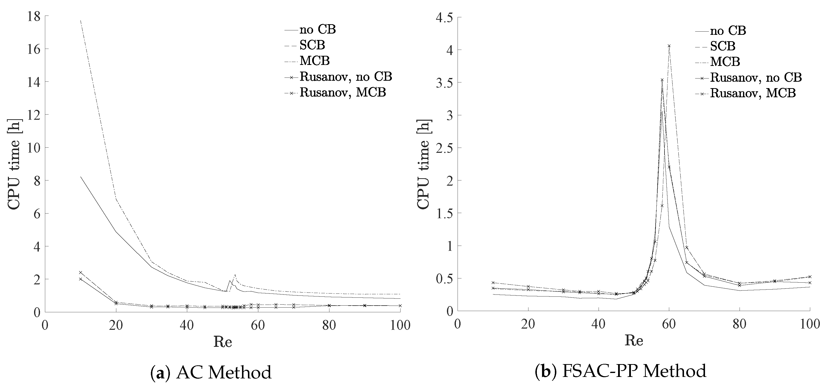
The computational cost is shown in Figure 6, which shows an interesting trend. The AC method is know to have slow convergence properties at low Reynolds numbers, see for example [22,23]. We see the same trend in Figure 6a, where the computational time required grows exponentially as the Reynolds number approaches zero. The non-CB and MCB scheme require substantially more CPU time than the SCB and RS-based approaches, however, the latter did not predict the bifurcation at all. The reason here is that the flow will always develop as a symmetrical flow, even for Reynolds number above Re. After the residuals have dropped to about , the numerical fluctuations become small enough so that the physical fluctuations can promote a different and more stable equilibrium position. At this stage, the reattachment point at the upper and lower wall start to interact with the upstream pressure at the convex corner points and slight physical fluctuations—which obtain their energy through the non-linear term—promote the change to a non-symmetrical flow pattern, which is also discussed by Oliveira [38]. Therefore, results obtained for the bifurcated state may in general require more computational time. At the critical Reynolds number, both the AC and FSAC-PP method peak in terms of the CPU time. It is here that the physical fluctuations become just important enough for the flow to register the change to a non-symmetrical state. At higher reynolds numbers, their effects may be felt stronger and earlier during the calculation which may force the bifurcation to occur earlier and thus with increasing Reynolds numbers, the computational time decreases again. When only considering the non-CB and MCB scheme of the AC method, which eventually bifurcate, it can be seen that the same simulation using the FSAC-PP method requires 2–3 times less CPU time sufficiently far away from the critical Reynolds number. This is consistent with findings of previous works in which it was highlighted that the FSAC-PP method generally performs faster than the AC method while retaining a high level of accuracy [22,23,28,30]. At Reynolds number close to zero, the computational savings are even more significant. This was one of the reasons the FSAC-PP method was developed in the first place, to overcome the stiff nature of the AC and Pressure Projection method for low Reynolds number flows, for example in microfluidic applications, see [23] for a detailed discussion. At the onset of bifurcation, however, the AC method seems to be slightly more cost efficient than the FSAC-PP method. This can be explained by the elliptic behaviour of the Poisson solver, where any pressure change is propagated through the domain instantaneously. These pressure waves require longer to be damped while the hyperbolic behaviour of the AC method induces less pressure waves and hence a converged solution is found quicker.
6. Conclusions
In this work, we presented results to predict the highly non-linear behaviour produced by the Navier–Stokes equations at low Reynolds numbers inside a channel with a sudden expansion. In particular, we investigated the sub- and super-critical range of Reynolds numbers where the flow bifurcates from a symmetric to a non-symmetric state. We investigated the performance of a non-characteristic-based (CB) scheme, single- and multi-directional characteristics-based scheme (SCB/MCB), as well as the Rusanov Riemann solver (RS) and combinations of these schemes and tested all approaches with the Artificial Compressibility (AC) and Fractional-Step, Artificial Compressibility with Pressure-Projection (FSAC-PP) method.
We found that only the non-CB and the MCB scheme were capable of predicting the bifurcation using the AC method where the RS-based approaches showed too much numerical dissipation to correctly predict the flow patterns. A significant difference between the SCB and MCB scheme could be observed in the AC method, where we showed that the multi-directional nature of the MCB scheme is required to predict the bifurcation at all. The added Rusanov RS showed too much numerical dissipation for the current approach to predict the bifurcation and similar results were obtained using the hybrid Rusanov and MCB scheme. In the FSAC-PP method, however, all schemes correctly predicted the symmetry breaking and overall showed better agreement with reference data in terms of the reattachment length. The incompressible flow method itself could overcome the inherent numerical dissipation of the Rusanov RS, as well as the SCB scheme which uses Godunov’s RS by default, showing that the mathematical classification of the method’s partial differential equations play a dominant role. The fully hyperbolic behaviour of the AC method was not always capable of capturing the bifurcation phenomena correctly while the mixed hyperbolic-elliptic equations of the FSAC-PP method ensured always a physically correct solution. This comes at a slightly increased computational cost near the bifurcation, however, sufficiently far away from the critical Reynolds number, the FSAC-PP method required 2–3 times less CPU resources compared to the AC method.
Aerospace applications are presented with flow features that are highly non-linear, as discussed in Section 1. The bifurcation shares many similarities to the onset to turbulence and predicting both phenomena correctly is mandatory to gain highly accurate computations in which stall, strong crossflow gradients and lift slope hysteresis are of interest. We have demonstrated here that the success of predicting non-linear flow features is not just scheme dependent, but the incompressible method used for the computation also plays a dominant role. The MCB scheme by itself showed that its multi-directional nature was capable of predicting non-linear phenomena correctly, regardless of the incompressible flow method used, while the SCB scheme was only capable of predicting correctly the flow phenomena when the FSAC-PP method was used. Although only laminar flows were investigated in this study, at higher Reynolds numbers, as is characteristic of aerospace applications, the flow becomes turbulent. In these flow regimes, the numerical dissipation produced by different schemes and RS becomes important. The Rusanov RS provides a sufficient amount of inherent numerical dissipation to tackle high Reynolds number turbulent flows. In future work, we will investigate the proposed framework for high Reynolds number flows, however, the framework present in the current study is directly applicable to such flows for aerospace applications.
Acknowledgments
The present research work was financially supported by the Centre for Computational Engineering Sciences at Cranfield University under the project code EEB6001R. The authors would like to acknowledge the IT support and the use of the High Performance Computing (HPC) facilities at Cranfield University, UK. We would also like to acknowledge the constructive comments of the reviewers of the Aerospace Journal.
Author Contributions
Tom-Robin Teschner, László Könözsy and Karl W. Jenkins contributed equally to this article.
Conflicts of Interest
The authors declare no conflict of interest.
Abbreviations
The following abbreviations are used in this manuscript:
| AC | Artificial Compressibility |
| CB | Characteristics-based |
| FSAC-PP | Fractional-Step, Artificial Compressibility with Pressure-Projection |
| FS-PP | Fractional-Step, Pressure-Projection |
| LES | Large-Eddy Simulation |
| MCB | multi-directional characteristics-based |
| RANS | Reynolds-averaged Navier–Stokes |
| RS | Riemann solver |
| SCB | single-directional characteristics-based |
References
- Mittal, S.; Saxena, P. Prediction of Hysteresis Associated with the Static Stall of an Airfoil. AIAA J. 2000, 38, 933–935. [Google Scholar] [CrossRef]
- Truong, K. Modeling Aerodynamics, Including Dynamic Stall, for Comprehensive Analysis of Helicopter Rotors. Aerospace 2016, 4, 1–24. [Google Scholar] [CrossRef]
- [-5]Traub, L. Semi-Empirical Prediction of Airfoil Hysteresis. Aerospace 2016, 3, 1–8. [Google Scholar] [CrossRef]
- Panaras, A. Turbulence Modeling of Flows with Extensive Crossflow Separation. Aerospace 2015, 2, 461–481. [Google Scholar] [CrossRef]
- Drikakis, D.; Rider, W. High-Resolution Methods for Incompressible and Low-Speed Flows; Springer: Heidelberg, Germany, 2005; ISBN 978-3-540-22136-4. [Google Scholar]
- Toro, E.F. Riemann Solvers and Numerical Methods for Fluid Dynamics; Springer: Heidelberg, Germany, 2009; ISBN 978-3-540-25202-3. [Google Scholar]
- Rusanov, V.V. Characteristics of the General Equations of Gas Dynamics. Noi Math. Math. Fiz. 1963, 3, 508–527. [Google Scholar] [CrossRef]
- Chorin, A.J. A Numerical Method for Solving Incompressible Viscous Flow Problems. J. Comput. Phys. 1967, 2, 12–26. [Google Scholar] [CrossRef]
- Drikakis, D.; Govatsos, P.A.; Papantonis, P.E. A Characteristic-based Method for Incompressible Flows. Int. J. Numer. Methods Fluids 1994, 19, 667–685. [Google Scholar] [CrossRef]
- Zienkiewicz, O.C.; Codina, R. A General Algorithm for Compressible and Incompressible Flow—Part I. The Split, Characteristic-Based Scheme. Int. J. Numer. Methods Fluids 1995, 20, 869–885. [Google Scholar] [CrossRef]
- Zienkiewicz, O.C.; Morgan, K.; Satya Sai, B.V.K.; Codina, R.; Vasquez, M. A General Algorithm for Compressible and Incompressible Flow—Part II. Tests on the Explicit Form. Int. J. Numer. Methods Fluids 1995, 20, 887–913. [Google Scholar] [CrossRef]
- Neofytou, P. Revision of the Characteristics-based Scheme for Incompressible Flows. J. Comput. Phys. 2007, 222, 475–484. [Google Scholar] [CrossRef]
- Su, X.; Zhao, Y.; Huang, X. On the Characteristics-based ACM for Incompressible Flows. J. Comput. Phys. 2007, 227, 1–11. [Google Scholar] [CrossRef]
- Razavi, S.E.; Zamzamian, K.; Farzadi, A. Genuinely Multidimensional Characteristic-based Scheme for Incompressible Flows. Int. J. Numer. Methods Fluids 2008, 57, 929–949. [Google Scholar] [CrossRef]
- Zamzamian, K.; Razavi, S.E. Multidimensional Upwinding for Incompressible Flows based on Characteristics. J. Comput. Phys. 2008, 227, 8699–8713. [Google Scholar] [CrossRef]
- Hashemi, M.Y.; Zamzamian, K. A Multidimensional Characteristic-Based Method for Making Incompressible Flow Calculations on Unstructured Grids. J. Comput. Appl. Math. 2014, 259, 752–759. [Google Scholar] [CrossRef]
- Hashemi, M.Y.; Zamzamian, K. Efficient and Non-Reflecting Far-Field Boundary Conditions for Incompressible Flow Calculations. Appl. Math. Comput. 2014, 230, 248–258. [Google Scholar] [CrossRef]
- Zamzamian, K.; Hashemi, M.Y. Multidimensional Characteristic-Based Solid Boundary Condition for Incompressible Flow Calculations. Appl. Math. Model. 2015, 39, 7032–7044. [Google Scholar] [CrossRef]
- Fathollahi, R.; Zamzamian, K. An Improvement for Multidimensional Characteristic-based Scheme by Using Different Selected Waves. Int. J. Numer. Methods Fluids 2014, 76, 722–736. [Google Scholar] [CrossRef]
- Razavi, S.E.; Adibi, T. A Novel Multidimensional Characteristic Modeling of Incompressible Convective Heat Transfer. J. Appl. Fluid Mech. 2016, 9, 1135–1146. [Google Scholar] [CrossRef]
- Razavi, S.E.; Hanifi, M. A Multi-Dimensional Virtual Characteristic Scheme for Laminar and Turbulent Incompressible Flows. J. Appl. Fluid Mech. 2016, 9, 1579–1590. [Google Scholar] [CrossRef]
- Könözsy, L. Multiphysics CFD Modelling of Incompressible Flows at Low and Moderate Reynolds Numbers. Ph.D. Thesis, Cranfield University, Cranfield, UK, 2012. [Google Scholar]
- Könözsy, L.; Drikakis, D. A Unified Fractional-Step, Artificial Compressibility and Pressure-Projection Formulation for Solving the Incompressible Navier–Stokes Equations. Commun. Comput. Phys. 2014, 16, 1135–1180. [Google Scholar] [CrossRef]
- Chorin, A.J. Numerical Solution of the Navier–Stokes Equations. Math. Comput. 22, 745–762. [CrossRef]
- Temam, R. Sur l’approximation de la Solution des Equations de Navier–Stokes par la Methode des pas Fractionnaires. Arch. Ration. Mech. Anal. 1969, 32, 377–385. [Google Scholar] [CrossRef]
- Könözsy, L.; Drikakis, D. A Coupled High-Resolution Fractional-Step Artificial Compressibility and Pressure-Projection Formulation for Solving Incompressible Multi-Species Variable Density Flow Problem at Low Reynolds Numbers. In Proceedings of the European Congress on Computational Methods in Applied Sciences and Engineering, Vienna, Austria, 10–14 September 2012. [Google Scholar]
- Könözsy, L.; Drikakis, D.; Ashcroft, M.; Dixon, A.; Perrson, J. Experimental and Numerical Investigation for Trapping and Positioning Cryogenic Propellants. In Proceedings of the 8th European Symposium on Aerothermodynamics for Space Vehicles, Lisbon, Portugal, 3–5 March 2015. [Google Scholar]
- Teschner, T.-R.; Könözsy, L.; Jenkins, K.W. Numerical Investigation of an Incompressible Flow over a Backward Facing Step Using a Unified Fractional-Step, Artificial Compressibility and Pressure-Projection (FSAC-PP) Method. In Proceedings of the MultiScience—XXX. microCAD International Multidisciplinary Scientific Conference, Miskolc, Hungary, 21–22 April 2016. [Google Scholar]
- Tsoutsanis, P.; Kokkinakis, I.; Ioannis, W.; Könözsy, L.; Drikakis, D.; Williams, R.J.R.; Youngs, D.L. Comparison of Structured- and Unstructured-Grid, Compressible and Incompressible Methods Using the Vortex Pairing Problem. Comput. Methods Appl. Mech. Eng. 2015, 293, 207–231. [Google Scholar] [CrossRef] [Green Version]
- Teschner, T.-R.; Könözsy, L.; Jenkins, K.W. On Godunov-Type Multi-Directional Characteristic-based Schemes for Hyperbolic Incompressible Flow Solvers. In Proceedings of the IV ECCOMAS Young Investigator Conference, Milan, Italy, 13–15 September 2017. [Google Scholar]
- Smith, K.; Teschner, T.-R.; Könözsy, L. On Approximate Riemann Solvers within the Concept of the Unified Fractional-Step, Artificial Compressibility and Pressure Projection (FSAC-PP) Method. In Proceedings of the MultiScience—XXX. microCAD International Multidisciplinary Scientific Conference, Miskolc, Hungary, 21–22 April 2016. [Google Scholar]
- Zucrow, M.J.; Hoffman, J.D. Gas Dynamics, Vol 1; John Wiley & Sons, Inc.: Hoboken, NJ, USA, 1976; ISBN 978-0471984405. [Google Scholar]
- Zucrow, M.J.; Hoffman, J.D. Gas Dynamics, Vol 2: Multidimensional Flow; John Wiley & Sons, Inc.: Hoboken, NJ, USA, 1977; ISBN 978-0471018063. [Google Scholar]
- Delaney, R.A. A Second-Order Method of Characteristics for Two-Dimensional Unsteady Flow with Application to Turbomachinery Cascades. Ph.D. Thesis, Iowa State University, Ames, IA, USA, 1974. [Google Scholar]
- Rusanov, V.V. The Calculation of the Interaction of Non-Stationary Shock Waves and Obstacles. USSR Comput. Math. Math. Phys. 1961, 1, 304–320. [Google Scholar] [CrossRef]
- Davis, S. Simplified Second-Order Godunov-Type Methods. SIAM J. Sci. Stat. Comput. 1988, 9, 445–473. [Google Scholar] [CrossRef]
- Roache, P.J. Perspective: A Method for Uniform Reporting of Grid Refinement Studies. J. Fluids Eng. 1994, 116, 405–413. [Google Scholar] [CrossRef]
- Oliveira, P.J. Asymmetric Flows of Viscoelastic Fluids in Symmetric Planar Expansion Geometries. J. Non-Newton. Fluid 2003, 114, 33–63. [Google Scholar] [CrossRef]
- Fearn, R.M.; Mullin, T.; Cliffe, K.A. Nonlinear Flow Phenomena in a Symmetric Sudden Expansion. J. Fluid Mech. 1990, 211, 595–608. [Google Scholar] [CrossRef]
- Teschner, T.-R.; Könözsy, L.; Jenkins, K.W. A Three-Stage Algorithm for Solving Incompressible Flow Problems. In Proceedings of the MultiScience—XXXI. microCAD International Multidisciplinary Scientific Conference, Miskolc, Hungary, 20–21 April 2017. [Google Scholar]
- Drikakis, D. Bifurcation Phenomena in Incompressible Sudden Expansion Flows. Phys. Fluids 1997, 9, 76–87. [Google Scholar] [CrossRef]
Figure 1.
Intersection of the characteristic surfaces with time level .

Figure 2.
Geometry of the channel with a sudden expansion. Boundary conditions are given for the inflow, outflow and solid (wall) boundary condition.
Figure 2.
Geometry of the channel with a sudden expansion. Boundary conditions are given for the inflow, outflow and solid (wall) boundary condition.

Figure 3.
Contour plots of the axial velocity component using a non-CB treatment.

Figure 4.
Velocity profiles at for the AC (top) and FSAC-PP (bottom) method using different combinations of CB schemes and the Rusanov Riemann solver at Re = 34.6 (left) and Re = 80 (right).
Figure 4.
Velocity profiles at for the AC (top) and FSAC-PP (bottom) method using different combinations of CB schemes and the Rusanov Riemann solver at Re = 34.6 (left) and Re = 80 (right).


Figure 5.
Bifurcation diagram for the AC (a) and FSAC-PP (b) method using different combinations of CB schemes and the Rusanov Riemann solver.
Figure 5.
Bifurcation diagram for the AC (a) and FSAC-PP (b) method using different combinations of CB schemes and the Rusanov Riemann solver.
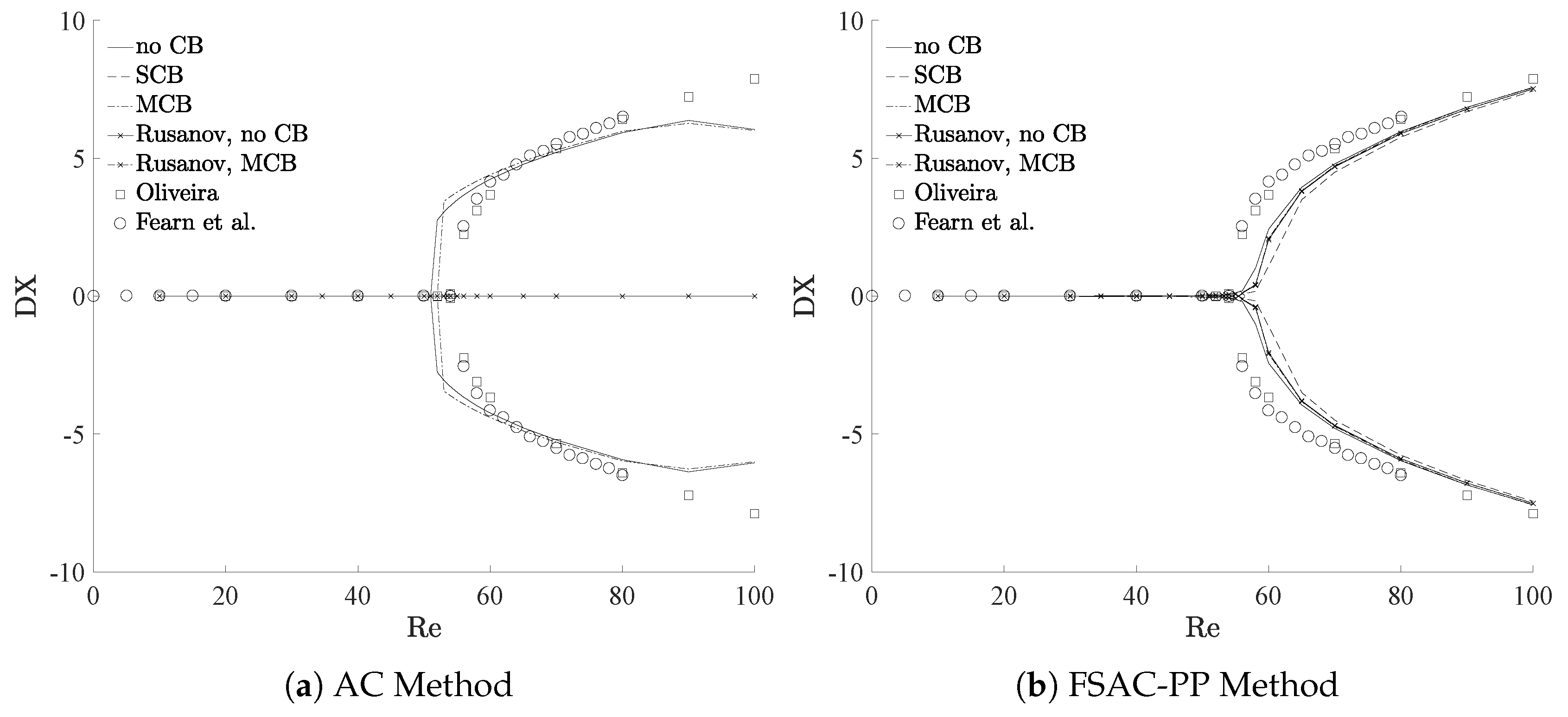
Figure 6.
Total number of iterations required for the AC (a) and FSAC-PP (b) method for different Reynolnds numbers.
Figure 6.
Total number of iterations required for the AC (a) and FSAC-PP (b) method for different Reynolnds numbers.


Table 1.
Grid dependency study for the AC and FSAC-PP method at a Reynolds number of Re = 30. The expected value of the reattachment length is as given by Oliveira [38].
Table 1.
Grid dependency study for the AC and FSAC-PP method at a Reynolds number of Re = 30. The expected value of the reattachment length is as given by Oliveira [38].
| Method | Cells | GCI (r1) | GCI (r2) | Time (h) | Iterations | ||
|---|---|---|---|---|---|---|---|
| AC | 1400 | 3.65448 | 3.65448 | - | - | 0.006 | 40,051 |
| 5600 | 3.92843 | 3.92843 | 0.3269 | 0.3269 | 0.13 | 222,404 | |
| 22,400 | 4.2131 | 4.2131 | 0.3167 | 0.3167 | 2.73 | 1,221,133 | |
| 89,600 | 4.40196 | 4.40196 | 0.2011 | 0.2011 | 32.2 | 2,768,606 | |
| Richardson Extrapolation | 4.4146 | 4.4146 | - | - | - | - | |
| FSAC-PP | 1400 | 2.78324 | 2.83458 | - | - | 0.003 | 11,534 |
| 5600 | 2.85779 | 2.87495 | 0.1223 | 0.0658 | 0.019 | 22,408 | |
| 22,400 | 2.9544 | 2.96133 | 0.1533 | 0.1367 | 0.22 | 58,896 | |
| 89,600 | 3.03597 | 3.03854 | 0.1259 | 0.1191 | 3.19 | 177,801 | |
| Richardson Extrapolation | 3.0414 | 3.0437 | - | - | - | - |
Table 2.
Convergence study for different level of convergence at a Reynolds number of Re = 30 based on the reattachment length and at the upper and lower wall.
Table 2.
Convergence study for different level of convergence at a Reynolds number of Re = 30 based on the reattachment length and at the upper and lower wall.
| Method | ||||||||
|---|---|---|---|---|---|---|---|---|
| AC | 3.28289 | 3.89382 | 4.00063 | 4.16895 | 4.20950 | 4.21217 | 4.21310 | |
| 3.28289 | 3.89382 | 4.00063 | 4.16895 | 4.20950 | 4.21217 | 4.21310 | ||
| FSAC-PP | 3.05442 | 2.97130 | 2.96041 | 2.96123 | 2.96134 | 2.96133 | 2.96133 | |
| 3.04702 | 2.96438 | 2.95348 | 2.95430 | 2.95441 | 2.95440 | 2.95440 |
Table 3.
and error norm of the velocity profiles for the AC method using different combinations of CB schemes and the Rusanov Riemann solver at Re = 34.6 and Re = 80.
Table 3.
and error norm of the velocity profiles for the AC method using different combinations of CB schemes and the Rusanov Riemann solver at Re = 34.6 and Re = 80.
| Re | No Rusanov RS | Rusanov RS | ||||
|---|---|---|---|---|---|---|
| No CB | SCB | MCB | No CB | MCB | ||
| 34.6 | [%] | 5.05 | 4.38 | 4.94 | 4.65 | 4.65 |
| [%] | 2.97 | 2.18 | 2.89 | 2.36 | 2.36 | |
| 80 | [%] | 6.43 | 41.31 | 7.14 | 41.19 | 41.19 |
| [%] | 3.75 | 25.10 | 4.19 | 24.87 | 24.87 | |
Table 4.
and error norm of the velocity profiles for the FSAC-PP method using different combinations of CB schemes and the Rusanov Riemann solver at Re = 34.6 and Re = 80.
Table 4.
and error norm of the velocity profiles for the FSAC-PP method using different combinations of CB schemes and the Rusanov Riemann solver at Re = 34.6 and Re = 80.
| Re | No Rusanov RS | Rusanov RS | ||||
|---|---|---|---|---|---|---|
| No CB | SCB | MCB | No CB | MCB | ||
| 34.6 | [%] | 4.10 | 4.98 | 4.19 | 4.05 | 4.03 |
| [%] | 1.96 | 2.57 | 2.03 | 1.93 | 1.91 | |
| 80 | [%] | 4.25 | 5.62 | 4.74 | 5.18 | 5.13 |
| [%] | 1.99 | 3.15 | 2.33 | 2.51 | 2.47 | |
Table 5.
Prediction of the reattachment length and and number of iterations required for convergence for different Reynolds numbers using the AC method for various combinations of CB schemes and the Rusanov Riemann solver.
Table 5.
Prediction of the reattachment length and and number of iterations required for convergence for different Reynolds numbers using the AC method for various combinations of CB schemes and the Rusanov Riemann solver.
| Re | No Rusanov RS | Rusanov RS | Oliveira [38] | ||||
|---|---|---|---|---|---|---|---|
| No CB | SCB | MCB | No CB | MCB | |||
| 10 | iteration | 3,631,653 | 690,039 | 4,532,716 | 696,382 | 696,476 | - |
| 2.655 | 1.130 | 2.634 | 1.117 | 1.117 | 1.211 | ||
| 2.655 | 1.130 | 2.634 | 1.117 | 1.117 | 1.211 | ||
| 20 | iteration | 2,113,766 | 163,702 | 1,547,448 | 166,414 | 166,411 | - |
| 3.387 | 1.968 | 3.364 | 1.936 | 1.936 | 2.111 | ||
| 3.387 | 1.968 | 3.364 | 1.936 | 1.936 | 2.111 | ||
| 30 | iteration | 1,221,133 | 107,248 | 785,612 | 106,580 | 106,591 | - |
| 4.213 | 2.879 | 4.194 | 2.828 | 2.828 | 3.080 | ||
| 4.213 | 2.879 | 4.194 | 2.828 | 2.828 | 3.080 | ||
| 40 | iteration | 791,709 | 100,955 | 478,125 | 100,464 | 100,460 | - |
| 5.085 | 3.824 | 5.070 | 3.753 | 3.753 | 4.075 | ||
| 5.085 | 3.824 | 5.070 | 3.753 | 3.753 | 4.075 | ||
| 50 | iteration | 568,705 | 91,784 | 330,816 | 91,432 | 91,429 | - |
| 5.990 | 4.785 | 5.985 | 4.697 | 4.697 | 5.080 | ||
| 5.990 | 4.785 | 5.985 | 4.697 | 4.697 | 5.081 | ||
| 52 | iteration | 858,132 | 91,683 | 318,747 | 90,572 | 90,572 | - |
| 4.330 | 4.978 | 6.169 | 4.886 | 4.886 | 5.279 | ||
| 7.089 | 4.978 | 6.169 | 4.886 | 4.886 | 5.285 | ||
| 54 | iteration | 630,303 | 91,897 | 476,622 | 90,803 | 90,803 | - |
| 4.088 | 5.172 | 3.838 | 5.076 | 5.076 | 5.445 | ||
| 7.369 | 5.172 | 7.452 | 5.076 | 5.076 | 5.523 | ||
| 56 | iteration | 553,873 | 92,342 | 430,348 | 91,269 | 91,273 | - |
| 3.939 | 5.366 | 3.749 | 5.266 | 5.266 | 4.440 | ||
| 7.604 | 5.366 | 7.663 | 5.266 | 5.266 | 6.678 | ||
| 58 | iteration | 533,040 | 97,869 | 403,268 | 96,932 | 96,928 | - |
| 3.839 | 5.561 | 3.683 | 5.457 | 5.457 | 4.107 | ||
| 7.814 | 5.561 | 7.857 | 5.457 | 5.457 | 7.208 | ||
| 60 | iteration | 515,231 | 99,678 | 383,592 | 98,563 | 98,556 | - |
| 3.770 | 5.755 | 3.635 | 5.648 | 5.648 | 3.935 | ||
| 8.008 | 5.755 | 8.040 | 5.648 | 5.648 | 7.609 | ||
| 70 | iteration | 455,579 | 101,927 | 328,784 | 100,829 | 100,832 | - |
| 3.629 | 6.732 | 3.550 | 6.605 | 6.605 | 3.669 | ||
| 8.843 | 6.732 | 8.844 | 6.605 | 6.605 | 9.019 | ||
| 80 | iteration | 411,266 | 104,035 | 304,704 | 104,958 | 104,951 | - |
| 3.626 | 7.713 | 3.562 | 7.566 | 7.566 | 3.658 | ||
| 9.553 | 7.713 | 9.538 | 7.566 | 7.566 | 10.060 | ||
| 90 | iteration | 388,146 | 110,098 | 292,355 | 109,346 | 109,341 | - |
| 3.668 | 8.697 | 3.610 | 8.529 | 8.529 | 3.708 | ||
| 10.039 | 8.697 | 9.876 | 8.529 | 8.529 | 10.930 | ||
| 100 | iteration | 365,681 | 110,430 | 295,891 | 109,700 | 109,701 | - |
| 3.730 | 9.683 | 3.676 | 9.493 | 9.493 | 3.781 | ||
| 9.771 | 9.683 | 9.681 | 9.493 | 9.493 | 11.660 | ||
Table 6.
Prediction of the reattachment length and and number of iterations required for convergence for different Reynolds numbers using the FSAC-PP method for various combinations of CB schemes and the Rusanov Riemann solver.
Table 6.
Prediction of the reattachment length and and number of iterations required for convergence for different Reynolds numbers using the FSAC-PP method for various combinations of CB schemes and the Rusanov Riemann solver.
| Re | No Rusanov RS | Rusanov RS | Oliveira [38] | ||||
|---|---|---|---|---|---|---|---|
| No CB | SCB | MCB | No CB | MCB | |||
| 10 | iteration | 68,164 | 88,652 | 77,805 | 85,234 | 76,780 | - |
| 1.218 | 1.160 | 1.199 | 1.211 | 1.212 | 1.211 | ||
| 1.217 | 1.161 | 1.198 | 1.211 | 1.211 | 1.211 | ||
| 20 | iteration | 63,567 | 77,596 | 71,278 | 76,451 | 70,299 | - |
| 2.052 | 1.960 | 2.030 | 2.049 | 2.050 | 2.111 | ||
| 2.049 | 1.958 | 2.028 | 2.047 | 2.048 | 2.111 | ||
| 30 | iteration | 58,896 | 68,241 | 64,767 | 67,870 | 63,793 | - |
| 2.961 | 2.839 | 2.936 | 2.958 | 2.960 | 3.080 | ||
| 2.954 | 2.834 | 2.930 | 2.953 | 2.955 | 3.080 | ||
| 40 | iteration | 54,291 | 61,483 | 58,382 | 61,441 | 58,369 | - |
| 3.902 | 3.747 | 3.874 | 3.897 | 3.901 | 4.075 | ||
| 3.888 | 3.758 | 3.862 | 3.887 | 3.891 | 4.075 | ||
| 50 | iteration | 72,955 | 57,272 | 62,362 | 66,594 | 64,421 | - |
| 4.866 | 4.705 | 4.836 | 4.856 | 4.861 | 5.080 | ||
| 4.829 | 4.682 | 4.807 | 4.830 | 4.836 | 5.081 | ||
| 52 | iteration | 103,038 | 68,241 | 887,76 | 94,788 | 91,491 | - |
| 5.068 | 4.866 | 4.994 | 5.054 | 5.060 | 5.279 | ||
| 5.013 | 4.898 | 5.035 | 5.017 | 5.023 | 5.285 | ||
| 54 | iteration | 160,834 | 98,874 | 134,456 | 143,614 | 139,714 | - |
| 5.190 | 5.094 | 5.239 | 5.200 | 5.207 | 5.445 | ||
| 5.279 | 5.048 | 5.176 | 5.257 | 5.262 | 5.523 | ||
| 56 | iteration | 323,916 | 158,368 | 243,044 | 260,922 | 257,718 | - |
| 5.333 | 5.221 | 5.342 | 5.368 | 5.374 | 4.440 | ||
| 5.522 | 5.299 | 5.461 | 5.475 | 5.480 | 6.678 | ||
| 58 | iteration | 878,294 | 334,541 | 768,416 | 865,548 | 901,939 | - |
| 5.084 | 5.362 | 5.377 | 5.415 | 5.405 | 4.107 | ||
| 6.095 | 5.534 | 5.802 | 5.805 | 5.825 | 7.208 | ||
| 60 | iteration | 355,946 | 888,435 | 481,042 | 514,272 | 486,624 | - |
| 4.427 | 5.051 | 4.641 | 4.655 | 4.628 | 3.935 | ||
| 6.861 | 6.149 | 6.688 | 6.700 | 6.726 | 7.609 | ||
| 70 | iteration | 114,816 | 126,413 | 119,971 | 127,121 | 125,149 | - |
| 3.734 | 3.782 | 3.779 | 3.785 | 3.782 | 3.669 | ||
| 8.531 | 8.278 | 8.499 | 8.475 | 8.485 | 9.019 | ||
| 80 | iteration | 91,835 | 94,097 | 92,946 | 99,882 | 98,683 | - |
| 3.653 | 3.650 | 3.679 | 3.681 | 3.679 | 3.658 | ||
| 9.622 | 9.416 | 9.618 | 9.572 | 9.579 | 10.060 | ||
| 90 | iteration | 96,853 | 95,949 | 97,232 | 114,014 | 105,340 | - |
| 3.676 | 3.656 | 3.696 | 3.703 | 3.702 | 3.708 | ||
| 10.525 | 10.346 | 10.539 | 10.480 | 10.486 | 10.930 | ||
| 100 | iteration | 106,408 | 109,105 | 119,534 | 108,770 | 102,731 | - |
| 3.749 | 3.705 | 3.762 | 3.754 | 3.753 | 3.781 | ||
| 11.308 | 11.147 | 11.336 | 11.263 | 11.269 | 11.660 | ||
© 2018 by the authors. Licensee MDPI, Basel, Switzerland. This article is an open access article distributed under the terms and conditions of the Creative Commons Attribution (CC BY) license (http://creativecommons.org/licenses/by/4.0/).
Share and Cite
MDPI and ACS Style
Teschner, T.-R.; Könözsy, L.; Jenkins, K.W. Predicting Non-Linear Flow Phenomena through Different Characteristics-Based Schemes. Aerospace 2018, 5, 22. https://doi.org/10.3390/aerospace5010022
AMA Style
Teschner T-R, Könözsy L, Jenkins KW. Predicting Non-Linear Flow Phenomena through Different Characteristics-Based Schemes. Aerospace. 2018; 5(1):22. https://doi.org/10.3390/aerospace5010022
Chicago/Turabian StyleTeschner, Tom-Robin, László Könözsy, and Karl W. Jenkins. 2018. "Predicting Non-Linear Flow Phenomena through Different Characteristics-Based Schemes" Aerospace 5, no. 1: 22. https://doi.org/10.3390/aerospace5010022
Note that from the first issue of 2016, this journal uses article numbers instead of page numbers. See further details here.