The Development of an Ordinary Least Squares Parametric Model to Estimate the Cost Per Flying Hour of ‘Unknown’ Aircraft Types and a Comparative Application ^†

Abstract

The development of a parametric model for the variable portion of the Cost Per Flying Hour (CPFH) of an ‘unknown’ aircraft platform and its application to diverse types of fixed and rotary wing aircraft development programs (F-35A, Su-57, Dassault Rafale, T-X candidates, AW189, Airbus RACER among others) is presented. The novelty of this paper lies in the utilization of a diverse sample of aircraft types, aiming to obtain a ‘universal’ Cost Estimating Relationship (CER) applicable to a wide range of platforms. Moreover, the model does not produce absolute cost figures but rather analogy ratios versus the F-16’s CPFH, broadening the model’s applicability. The model will enable an analyst to carry out timely and reliable Operational and Support (O&S) cost estimates for a wide range of ‘unknown’ aircraft platforms at their early stages of conceptual design, despite the lack of actual data from the utilization and support life cycle stages. The statistical analysis is based on Ordinary Least Squares (OLS) regression, conducted with R software (v5.3.1, released on 2 July 2018). The model’s output is validated against officially published CPFH data of several existing ‘mature’ aircraft platforms, including one of the most prolific fighter jet types all over the world, the F-16C/D, which is also used as a reference to compare CPFH estimates of various next generation aircraft platforms. Actual CPFH data of the Hellenic Air Force (HAF) have been used to develop the parametric model, the application of which is expected to significantly inform high level decision making regarding aircraft procurement, budgeting and future force structure planning, including decisions related to large scale aircraft modifications and upgrades.

1. Introduction

At the present environment of decreasing defence budgets, obtaining the right balance among the components of force structure, modernization, readiness and sustainability of an Air Force is extremely challenging and requires careful analysis of the cost data. Cost Per Flying Hour (CPFH) is the main metric that many Air Forces are using to develop operating and support budgets and is defined as [1]:

$$\mathrm{CPFH}=\frac{\mathrm{Total}\mathrm{O}\&\mathrm{S}\mathrm{Costs}}{\mathrm{Total}\mathrm{Flying}\mathrm{Hours}}$$

(1)

Air Forces and aircraft operation organizations across the world use CPFH estimates mainly to budget resources to achieve aircrew proficiency. Other potential uses of CPFH estimates are for flying hour reimbursable billing rates, in other words estimating how much other governmental agencies, foreign militaries and any other customer should be charged on a per-flying-hour basis, given the variety of services an Air Force owned fleet can offer (search and rescue for civilians, aerial fire-fighting, provision of air patrol and flight training to allied nations, participation in flight displays, to name a few). Last but not least, CPFH estimates are essential in comparing the Operational and Support (O&S) costs of different aircraft programs. CPFH estimates are then multiplied by projected flying hours and the projected budget requirements feed the decision-making process of the organization. However, actual costs do not always change to the extent predicted by this multiplicative application of the CPFH estimates. Selected prior work which deals with the complexities, the challenges, the strengths and the weaknesses of the CPFH method is discussed below.

Hildebrandt and Sze [2] have conducted regression studies, which relate multiple system’s flying hours to several different elements of O&S cost and they found, in general, that O&S costs increase less than proportionally with flying hours. Their study has developed Cost Estimating Relationships (CERs), which relate the O&S cost with aircraft design features and operating tempo variables and as such, these relationships might be useful for estimating the O&S cost of an acquisition program during the early stages of the planning, programming and budgeting cycle. Using data from 1993 to 1996, Sherbrooke [3] has challenged the hypothesis that higher flying hour numbers lead to higher aircraft spares demand. By linking data from the supply database with the United States Air Force (USAF) core automated maintenance database, he has concluded that higher aircraft utilization rates tend to require less maintenance. Another significant finding of his work was that short training missions in which the pilots pulled as many as eight G’s had three times as many depot-level reparable ‘demands’ per sortie as long cross-country sorties.

Wallace et al. [4] have analysed C-5B fleet data during the Operation Desert Storm and C-17, KC-135 and F-16C fleet data during the 90’s operations in Kosovo and they have concluded that:

• The proportional CPFH model works: When nothing changes in the way an aircraft fleet flies (and rests) from one period to the next. It is then perfectly reasonable to use flying hours as a predictor for removal-causing failures. When fight behaviour does not change, the failure rate from each potential cause of failures remains constant.
• The proportional CPFH model fails: When a fleet of aircraft significantly changes its flight behaviour from one time interval to the next. An example of this is the wartime surge (flying hours increase dramatically but landings remain the same) and this is a typical case in which flying hours and the other factors that affect failures begin to diverge.

In a similar work which was carried out by Lee [5], a physics-based model has been developed that considered the ground equipment, flying hours and take-off/landing cycles to predict removals. The model has been applied to the Gulf War C-5B fleet data and it has provided more accurate results than the proportional CPFH model for the Gulf War surge.

Laubacher [6] has researched forecasting techniques for various helicopter types of the USAF, with an objective to reduce the differences between forecasted budgets and actual expenses. A similar study for various helicopter types of the United States Army has been conducted by Hawkins [7]. Armstrong [8] has analysed F-15 fleet data to estimate an incremental, rather than average CPFH. Hess [9] has evaluated the method used by the USAF to estimate the Flying Hour Program costs and introduced new methods to forecast future costs. His findings suggest that the assumption of a linear relationship between cost and flying hours is not appropriate.

Knowing the possible factors that cause operational and maintenance costs to fluctuate may allow for better predictions of the cost of the Flying Hour Program of an Air Force. Hawkes and White [10] investigated the predictive ability of many diverse variables such as aircraft age, average sortie duration, base location, utilization rate and engine type among others. Utilization rate, base location, block and engine type appeared to accurately predict an F-16 C/D fighter wing CPFH. Both regression models of their study are sensitive to utilization rates and that they inversely affect the CPFH, which is in good agreement with previous studies [3,4,5]. The modern F-16 blocks also decrease the cost of flying, generally older technology is more expensive to maintain. Hawkes and White [11] have also investigated the relationship between the aircraft age and ownership CPFH cost growth from seventy-four different airframes in the USAF inventory. Their findings suggest that very young and very old aircraft platforms exhibit higher levels of cost growth and variability, the magnitude though of the cost growth and variability for old aircraft platforms is almost equal to that of young aircraft. By examining the empirical relationship between multiple USAF system’s expenditures, flying hours and fleet sizes, Unger’s [12] research has suggested a more sophisticated way to think about USAF costs than is currently used. A fixed-plus-variable cost structure has been proposed in which the expenditures do not increase nor decrease in proportion to flying hours. Unger concludes with the policy implications of his research findings, noting that current USAF budgeting methods likely overestimate funding requirements when flying hours increase and underestimate requirements when flying hours decrease.

The discussion above highlights that the accuracy of a CPFH estimate is of paramount importance, given its use as a main decision-making tool at the upper echelons of the hierarchy of the organization. Error in the cost estimates has been identified as a causal factor in cost overruns and as studies have shown, cost overruns challenge fiscal management in the United States Department of Defense (US DoD) [13,14]. As a knock-on effect, they may also lead to funding instability in those programs that did not experience cost overruns but were affected by re-programming of funds. This instability in funding only further exacerbates cost overruns [15].

2. Materials and Methods

During the procurement process of an aircraft platform, there is an emphasis in affordability and cost management issues. Potential buyers can be always offered reliable estimates for the O&S costs of an aircraft platform which has been in operation and has reached its ‘fleet maturity’ stage. This is not possible though in the case of comparing and evaluating new (‘unknown’) aircraft platforms, therefore the decisions should be based, if possible, to cost estimates the variables of which are known at the time of the procurement process. This is one of the main objectives of the paper, to develop a CER which will enable an analyst to carry out a timely and reliable O&S cost forecast, despite the lack of actual data from the utilization and support life cycle stages of the platform, during which the largest portion of the Life Cycle Cost (LCC), nearly 60%, is incurred [16]. As such, aircraft’s physical and performance characteristics and parameters which are known very well in advance at the aircraft’s conceptual design phase, are being researched on the present work as potential variables of an O&S parametric cost estimation model. An introductory demonstration of this concept has been presented by one of the authors at the 2016 International Training Symposium of the ICEAA [17].

2.1. The Parametric Estimation Technique

The parametric or ‘top-down’ technique is a relatively fast and inexpensive estimating tool. Properly applied, it may provide reliable predictions and, most important, timely estimates. According to ISPA/SCEA Parametric Handbook [18]:

Parametric estimating is a technique that develops cost estimates based upon the examination and validation of the relationships which exist between a project’s technical, programmatic and cost characteristics as well as the resources consumed during its development, manufacture, maintenance, and/or modification. Parametric models can be classified as simple or complex. Simple models are cost estimating relationships (CERs) consisting of one cost driver. Complex models, on the other hand, are models consisting of multiple CERs, or algorithms, to derive cost estimates.

The parametric technique is applicable during the early stages of a system’s life cycle, amidst analogy and engineering estimating techniques (Figure 1) [19]:

The parametric technique uses regression analysis for estimating the relationships among variables. Regression analysis helps an analyst to understand how the typical value of the dependent variable (response or criterion variable) changes when any one of the independent variables (predictors or explanatory variables) is varied, while the other independent variables are held fixed.

2.2. The Strengths and Weaknesses of the Parametric Estimation Technique

The implementation of the parametric technique is a blended process and the interpretation of the results has to be done with extreme caution. An analyst should always consider the following strengths and weaknesses of the parametric technique:

Strengths:

• It does not require actual and detailed cost information about a new system. Compared to the engineering or ‘bottom-up’ cost estimating technique, it requires less data, time and resources.
• It may reveal strong CERs between cost and Reliability-Maintainability-Supportability (RMS) metrics [20], thus helping to optimize maintenance and logistic procedures.
• A parametric model can be easily adjusted when the main cost drivers change. The CERs may be easily updated and sensitivity analysis may be applied.
• It is a sound statistical process and can be objectively validated.
• The uncertainty of the estimate can be quantified, allowing cost risk analysis.
• There are many available COTS parametric tools. Additionally, general-purpose statistical packages support the parametric technique.

Weaknesses:

• It is a rigorous statistical technique (uses regression analysis).
• CERs are often considered ‘black boxes,’ especially if they derive from COTS tools with unknown data libraries, and/or if the CER mathematical expression cannot be logically explained.
• Appropriate data adjustments might be required before the analysis, depending on the selected regression method (OLS, OLS-Log space, MUPE, ZMPE). Also, standard error adjustments for sample size and relevance might be required [21].
• CERs must be frequently updated to ensure validity.
• The validity of the PI and CI heavily depends on the residuals diagnostics.
• The decision makers may feel uncomfortable to base their final decision on a parametric estimate (probably they will not be statisticians).
• Wide-ranging PI or CI may render the estimate useless; why not use the ‘rule of thumb’ instead?

2.3. The Development of the Parametric Model

The relationship between historical CPFH and specific aircraft characteristics is investigated with an objective to identify a strong CER that will be used to estimate the hypothetical CPFH for an ‘unknown’ aircraft. Typically, the CPFH includes the following six main cost categories [16] according to the O&S cost element structure: Unit-level manpower, unit operations, maintenance, sustaining support, continuing system improvements and indirect support. Since the purpose of the presented parametric model is the assessment of the relationship between cost and technical or performance characteristics, the ‘indirect support’ cost category is excluded from the analysis.

The Fiscal Year (FY) 2013 CPFH data from the Hellenic Air Force (HAF) aircraft fleet have been used as input for the developed parametric model (

Table 1. HAF fixed and rotary wing aircraft types used for the development of the parametric model and related CPFH data for FY 2012, 2013 and 2018. (CPFH data for fighter aircraft is classified-publication is restricted. It includes the contribution of the ‘indirect support’ cost category. Data retrieved by various published issues of the Official Governmental Gazette of Greece (OGGG)).

Aircraft/Helicopter Type	CPFH (FY 2012, €)	CPFH (FY 2013, €)	CPFH (FY 2018, €)
Helicopters
B-212	10,089.9	3133.63	2297.00
AS-322C1	3142.43	3352.00	3583.64
AB-205	3790.32	3505.24	2479.77
A-109E	2800.21	2678.12	1788.13
Transport aircraft
C-130H/B	7370.88	7312.81	5887.34
C-27J	3174.90	4088.80	9114.23
Airborne Early Warning & Control aircraft
EMB-145H	9226.77	7570.15	4292.80
VIP aircraft
EMB-135	3545.58	4904.08	3162.17
Gulfstream V	3192.92	5537.09	3514.70
Training aircraft
T-41	3415.60	1449.12	1314.07
T-6A	1794.40	1839.08	2127.99
T-2	4206.68	4240.92	5154.07
Fire-fighting aircraft
CL-215	9807.82	8858.95	7117.25
CL-415	9508.46	6690.70	10,696.98
PZL	2492.69	1712.34	2884.25
Fighter aircraft
F-16C/D	Classified	Classified	Classified
F/RF-4E	Classified	Classified	Classified
M2000/-5	Classified	Classified	Classified
A-7H	Classified	Classified	Classified

). The Ministry of National Defence of Greece restricts the publication of the CPFH data for the fighter jet fleet, CPFH data though for other than fighter jet aircraft types are publicly available without any restriction. CPFH data of Table 1 includes the contribution of the ‘indirect support’ cost category which, as mentioned previously, was excluded from the present study.

In more detail, the 2012 CPFH Issue of the OGGG has been based on O&S data collected during the FY 2011, the 2013 CPFH Issue of the OGGG has been based on O&S data collected during the FY 2012 and the 2018 CPFH Issue of the OGGG has been based in analysis of O&S data collected during the FY 2015. At any point in time, the most recently published at that particular point in time CPFH Issue of the OGGG is used to feed the decision making of the Ministry of National Defence of Greece.

The 2013 CPFH Issue of the OGGG, which have been used for the development of the parametric model, is considered as having more reliable data than that of 2012, as the Ministry has transitioned from 2012 to a more GAO-streamlined [22] procedure for categorizing and analysing the cost input data. It was deemed necessary to exclude the contribution of the ‘indirect support’ cost category when developing the parametric model, as this category is influenced by extrinsic factors (institutional framework, organizational structure, integrated logistic support policies to name a few). As a matter of fact, the ‘indirect support’ cost category portion in HAF aircraft types ranges from 5% up to 50% of the CPFH, depending on these extrinsic factors.

The HAF fire-fighting fleet (CL-215, CL-415) case can provide some evidence to support our decision to exclude the ‘indirect support’ cost category. As observed from Table 1 (data including ‘indirect support’ cost), column ‘CPFH FY 2018,’ the CPFH of the CL-415 seems to be considerably higher than the CL-215 CPFH. It is worth noting that the CL-415, as opposed to CL-215, is a contemporary aircraft with enhanced reliability and maintainability provisions, equipped with very fuel efficient, latest technology turboprop engines. The paradox in the CPFH difference has to do with the fact that the CL-415 squadron experiences a higher ‘indirect support’ cost than the CL-215 squadron does. Almost the entire structure of 113th Wing supports the CL-415 squadron; on the contrary, the CL-215 squadron belongs in the organizational chart of 112th Wing, which supports other squadrons as well. Thus, in the case of 112th Wing, the ‘indirect support’ cost is allocated to multiple aircraft types (generally, each HAF Wing supports multiple aircraft squadrons and/or aircraft types [23]). Nevertheless, if the ‘indirect support’ cost is excluded, CL-415 experiences lower CPFH than the CL-215, which makes more sense for the comparative purpose of the development of the parametric model.

A generic view of the constraints/requirements and the parametric model performance is presented at the

Table 2. Generic view of the constraints/requirements and the parametric model performance.

Constraints and Requirements	Model Performance
Use the sample of 22 aircraft types operated by the HAF.	Satisfactory.
Use the appropriate cost information.	Satisfactory: Official FY 2013 CPFH data was used, excluding the ‘indirect support’ cost category.
Use cost drivers (independent variables) that are easily accessible and quantifiable.	Satisfactory: The cost drivers are aircraft physical and performance characteristics.
The model must be as less complex as possible and include no more than two cost drivers.	Satisfactory: The selected model includes two independent variables.
The model should be statistically significant at the 5% level.	Satisfactory: $p-value<0.01$
The model should capture at least 75% of the CPFH variance.	Satisfactory: $R_{adj}^2=0.82$
The model’s confidence and prediction intervals must be valid.	Satisfactory: The residuals do pass all the appropriate tests.
The model’s mathematical expression should make sense.	Satisfactory: The model suggests that the aircraft empty weight and the engine SFC correlate positively with the CPFH.

. The variables used for the analysis are shown at the

Table 3. The variables used for the analysis. In most cases, the log-transformations contributed to the creation of linear simple CERs versus the LogCPFH (Figure 2).

Variables	Variable Trans-Formation	Transformed Variable Notation	Assessment Tests * for Linearity among Variable and LogCPFH (‘Ø’ Indicates p-Value < 0.05)
			Test 1 a	Test 2 b	Test 3 c	Test 4 d	Test 5 e
Dependent
CPFH, €/h	Log	LogCPFH
Independent
Length (longitudinal axis), ft	Log	LogLENGTH	Ø			Ø
Empty weight, lb	Log	LogEMPTY
MTOW, lb	Log	LogMTOW
Max SFC, lb/(lbf∙h) or lb/(hp∙h)	Log	LogSFC
Max speed, km/h	Log	LogSPEED
Ceiling, ft	×10−4	AdjCEIL

* ^a: Global stat, ^b: Skewness, ^c: Kurtosis, ^d: Link Function, ^e: Heteroscedasticity.

.

The variables used for the analysis are shown at the Table 3.

Work done by Bryant ([24], Table 2, page 10) offers an overview of independent variables used in previous CPFH research. The variables are grouped in four distinct groups, namely ‘aircraft characteristics,’ ‘operational factors,’ ‘economic factors’ and ‘environmental factors.’ The most frequently used independent variables by the researchers are ‘average aircraft age’ (belonging to the ‘aircraft characteristics’ group) and ‘utilization rate’ (belonging to the ‘operational factors’ group), which also reflect the fact that the CPFH research efforts are mainly channelled to find answers to policy hypotheses which are questioning the effects of the aircraft fleet aging and utilization. Instead, the present study aims to provide a ‘universal’ CER applicable to a wide range of platforms, which can be used at the very early development stages of the ‘new’ aircraft design and, as such, the independent variables are concentrated to aircraft design and performance characteristics. Moreover, in most cases, the values of the variables are unclassified and they are readily available online, something that enhances the usability of the developed model.

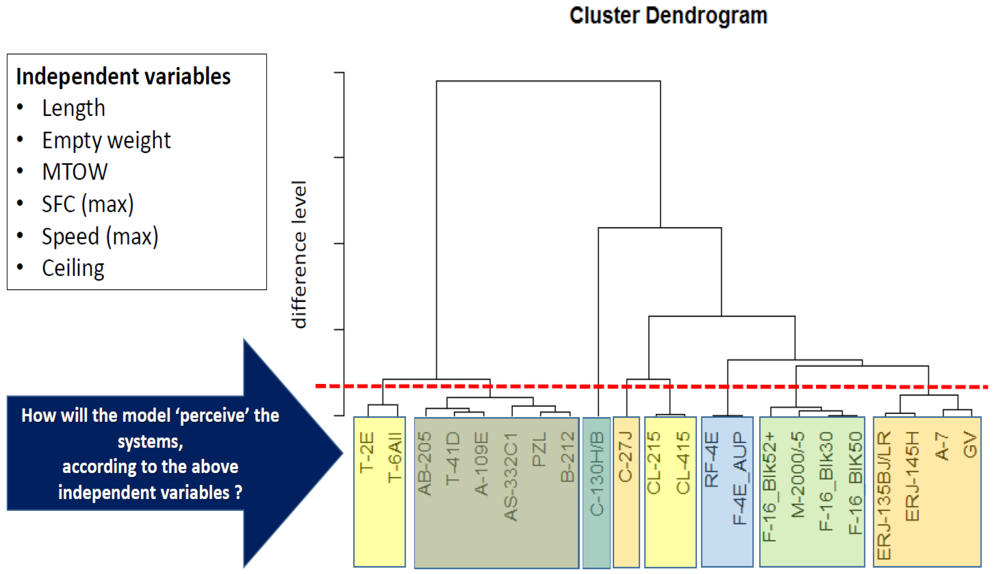
Figure 3 offers an overview of the way that the systems are being classified, based on the selected independent variables and depending on the desired systems similarity level. Because the selected independent variables serve as system identifiers, it is important to examine if the systems are perceptible in a realistic way and identified as ‘different’ or ‘similar’ through the regression process. The vertical axis of the cluster dendrogram in Figure 3 corresponds to the level of ‘resolution’ of the sample’s ‘image.’ The ‘resolution’ is tied to the independent variables, which serve as system identifiers.

For example, the red horizontal dashed line in Figure 3 corresponds to the selection of a low difference level (high ‘resolution’). This line cuts 8 branches of the dendrogram, meaning that the 22 different systems are identified and classified as 8 different entities (clusters), at the selected difference level. Specifically, the systems are grouped as follows: The 1st cluster includes two training aircraft (T-2E, T-6A II); the 2nd cluster includes the rotary wing platforms (AB-205, A-109E, AS-332C1, B-212) plus two light fixed-wing, single reciprocating engine, aircraft (T-41D, PZL); the 3rd cluster includes the four-engine transporter C-130H/B; the 4th cluster includes the lighter, two-engine transporter C-27J; the 5th cluster includes the two fire-fighting aircraft (CL-215, CL-415); the 6th cluster includes the two-engine supersonic jet fighter (F/RF-4E); the 7th cluster includes the single-engine supersonic jet fighters (F-16 blocks 30/50/52+, M2000/-5); the 8th cluster includes the VIP and early warning subsonic jet aircraft (ERJ-135BJ/LR, ERJ-145H, GV) plus the A-7H single-engine subsonic jet fighter. Apart from a few pitfalls, the classification of the systems according to the aforementioned clusters seems quite realistic.

Prior to the CPFH Log-transformation, the sample’s actual CPFH was multiplied by a positive real c, such that the selected model will estimate CPFH = 1 for the F-16C/D Block 52+. The F-16’s CPFH was chosen as the reference point for relative comparisons against other system’s CPFH. As a result, the model estimates the CPFH of any aircraft type times the F-16 mean CPFH. Analysts may use analogy to turn the model’s outputs into absolute CPFH estimates, by choosing a known system as their reference and multiplying its actual CPFH by the model’s output.

The pairwise assessment of the selected independent variables reveals multicollinearity issues. Two or more independent variables may be highly correlated, for example LogEMPTY and LogMTOW, meaning that one can be linearly estimated from the others with a substantial degree of accuracy. A parametric model should not include strongly correlated independent variables, because its predictive ability will decrease. The Pearson correlation matrix (Figure 4) offers an overview of the existing correlations among the transformed variables. Figure 5 shows examples of multicollinearity amongst various variables.

2.4. Selection of the Optimal CER

As seen in Figure 4, the highest correlation coefficient between LogCPFH and the independent variables is r = 0.83. Therefore, LogMTOW would be the best choice for developing a simple CER. Unluckily, this model does not comply at least with one of the requirements in Table 2, which is: R²_adj ≥ 0.75 (indeed, r² = 0.83² = 0.69 < 0.75).

The next step is to investigate all possible complex CERs with two independent variables, including their interaction, of the form:

$$Y={\beta }_0+{\beta }_1{X}_i+{\beta }_2{X}_j+{\beta }_3{X}_i{X}_j$$

(2)

where ${\beta }_0,{\beta }_1,{\beta }_2,{\beta }_3$ are the model’s coefficients and $i,j\in \left\{1,2,\dots ,6\right\}$, $i\ne j$. After performing stepwise regression on all possible (2 out of 6 = 15) models with two independent variables, as shown in Equation (2), the following model is chosen, according to the AIC as the measure of the CERs relative quality:

$$LogCPFH=-4.95006+0.4751LogEMPTY+0.42793LogSFC$$

(3)

Notably, the two selected independent variables do not correlate significantly (Figure 4 and Figure 6), so there is no multicollinearity in the selected model. Also, the interaction of the two independent variables is not significant, hence the term ${\beta }_3{X}_i{X}_j$ is omitted from the right hand of the equation.

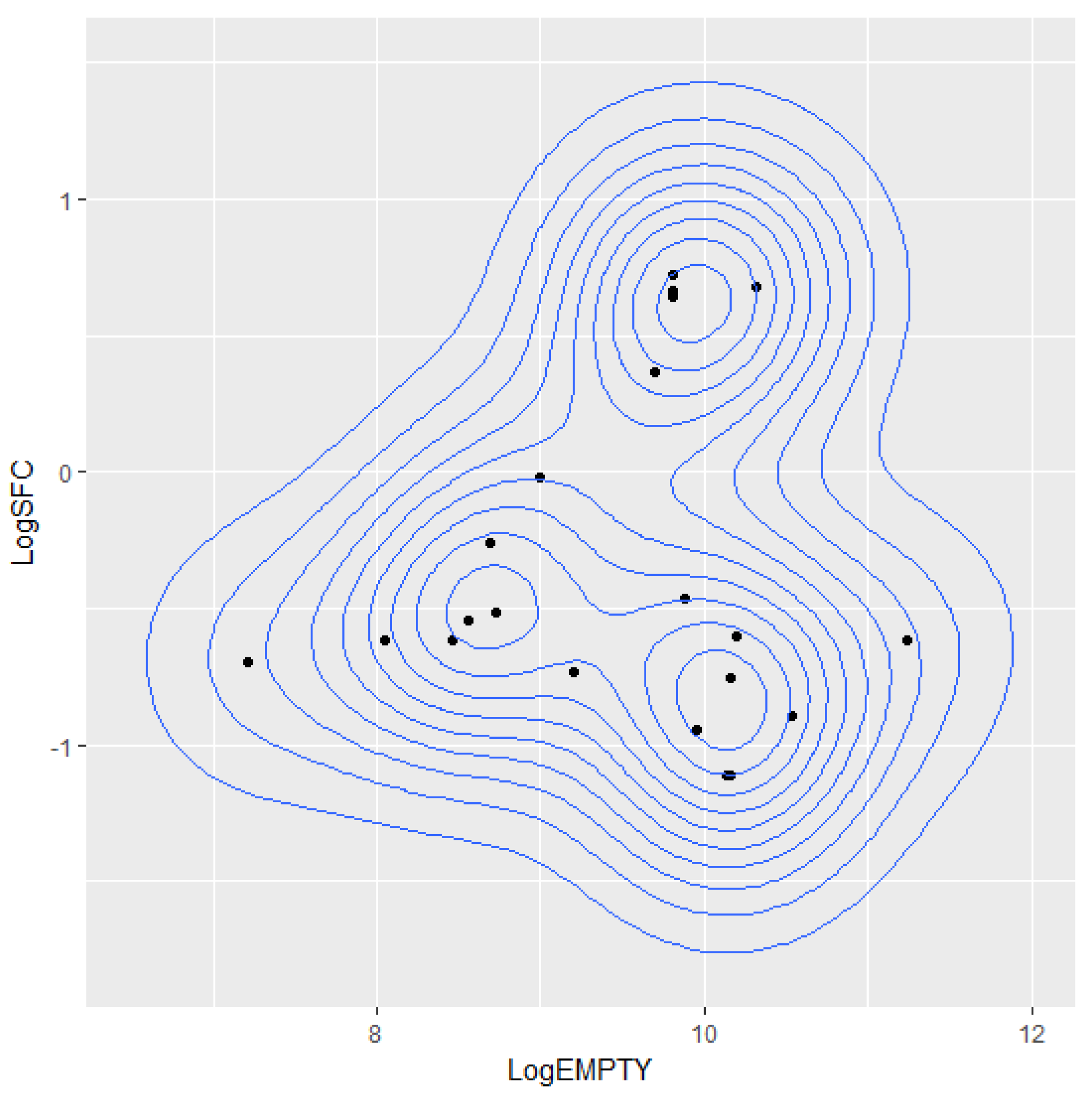
The selected model explains a remarkable 82.15% of the LogCPFH variance, while the intercept, LogEMPTY and LogSFC have significant explanatory power at the 5% significance level. The assumptions of model’s linearity are not rejected at the 5% significance level. Moreover, there is a statistically strong indication that no power transformation is required on LogCPFH.

Table 4. Model summary and ANOVA.

Model Selection
Start: AIC = −56.02
LogCPFH ~ LogEMPTY * LogSFC
	Df	Sum of Sq	RSS	AIC
LogEMPTY:LogSFC	1	0.040019	1.2384	−57.298
<none>			1.1984	−56.021
Step: AIC = −57.3
LogCPFH ~ LogEMPTY + LogSFC
	Df	Sum of Sq	RSS	AIC
<none>			1.2384	−57.298
−LogSFC	1	1.5185	2.7569	−41.692
−LogEMPTY	1	4.1550	5.3934	−26.929
Residuals
Min	1Q	Median	3Q	Max
−0.42125	−0.08515	−0.02154	0.09199	0.50650
Coefficients
	Estimate	Std. Error	t value	Pr(>|t|)
(Intercept)	−4.95006	0.57456	−8.615	5.48 × 10−8
LogEMPTY	0.47510	0.05951	7.984	1.73 × 10−7
LogSFC	0.42793	0.08866	4.827	0.000117
Residual standard error: 0.2553 on 19 degrees of freedom Multiple R-squared: 0.8385, Adjusted R-squared: 0.8215 F-statistic: 49.31 on 2 and 19 DF, p-value: 3.009 × 10−8
Correlation of Coefficients
	(Intercept)		LogEMPTY
LogEMPTY	−0.99
LogSFC	0.17		−0.13
Analysis of Variance Table
Response: LogCPFH
	Df	Sum Sq	Mean Sq	F value	Pr(>F)
LogEMPTY	1	4.9099	4.9099	75.327	4.895 × 10−8
LogSFC	1	1.5185	1.5185	23.296	0.0001172
Residuals	19	1.2384	0.0652
---
bcnPower Transformation to Normality
Estimated power, lambda
	Est Power	Rounded Pwr	Wald Lwr Bnd	Wald Upr Bnd
Y1	−1.2543	1	−5.4661	2.9574
Location gamma was fixed at its lower bound
	Est gamma	Std Err.	Wald Lower Bound	Wald Upper Bound
Y1	0.1	NA	NA	NA
Likelihood ratio tests about transformation parameters
		LRT	Df	pval
LR test, lambda = (0)		0.3258308	1	0.5681244
LR test, lambda = (1)		1.0123004	1	0.3143524
Assessment of the Linear Model Assumptions
		Value	p-value	Decision
Global Stat		0.776499	0.9416	Assumptions acceptable.
Skewness		0.593439	0.4411	Assumptions acceptable.
Kurtosis		0.001988	0.9644	Assumptions acceptable.
Link Function		0.177909	0.6732	Assumptions acceptable.
Heteroscedasticity		0.003163	0.9552	Assumptions acceptable.

shows the regression analysis details obtained from R software (v5.3.1, released on 2 July 2018) and Figure 6 shows a 2D density plot (log-scale) for the model’s independent variables.

2.5. Residuals Diagnostics

Getting valid prediction or confidence intervals relies on the assumptions that the residuals are normal with mean zero, have constant variance and no autocorrelations. The residuals of the selected model pass all the necessary tests (

Table 5. Summary of residuals diagnostics.

Test	Null Hypothesis	p-Value	Reject the Null Hypothesis at the 5% Significance Level?
Shapiro-Wilk normality test	Normality	0.161	NO
Breusch-Pagan test for heteroscedasticity	Constant variance	0.332	NO
Durbin-Watson test for autocorrelation	Randomness	0.302	NO
Two-sided t-test with Bonferroni adjustment	No outliers	0.714	NO

).

The residual plots (Figure 7) offer some additional insight, following the tests in Table 5. The histogram indicates normality for the residuals; there are a few high-discrepancy observations (candidate outliers) shown in the boxplot, however the respective test in Table 5 supports the null hypothesis that there are no outliers. The residual plots versus the fitted values indicate absence of curvature pattern and presence of constant variance, supported by the minor slope in the spread-level plot; furthermore, no significant autocorrelation is evident in the respective plots. There are also a few high-leverage observations, however no hat value exceeds the empirical limit for small samples (3 times the hat values mean). The studentized residuals seem to follow the theoretical student-t distribution, as shown in the Q-Q plot.

Observation no.14 needs further attention as being influential for the model, since its Cook’s distance exceeds the empirical cut-off limit. This data point corresponds to the C-130H/B, which is the heaviest aircraft within the sample (high-leverage observation); additionally, the model overestimates to a great degree the C-130H/B’s actual CPFH (high discrepancy observation). Excluding observation no.14 from the analysis would trigger a vicious cycle of consecutive exclusions, diminishing the size of the sample. Because the sample size is small, we decided not to exclude any observation from the regression analysis.

The construction of prediction or confidence intervals requires the residuals standard error and degrees of freedom (provided in Table 4), as well as the hat matrix. For any given input ${\mathbf{X}}_0^{\mathbf{T}}=\left[1,LogEMPT{Y}_0,LogSF{C}_0\right]$, the hat matrix $\mathbf{P}\equiv {\mathbf{X}}_0^{\mathbf{T}}{\left({\mathbf{X}}^{\mathbf{T}}\mathbf{X}\right)}^{-1}{\mathbf{X}}_0^{}$ can be calculated using the following information obtained from the sample:

$${\left({\mathbf{X}}^{\mathbf{T}}\mathbf{X}\right)}^{-1}=\left[\begin{array}{ccc}5.0647305& -0.5216059& 0.1365213\\ -0.5216059& 0.0543257& -0.0104403\\ 0.1365213& -0.0104403& 0.1205977\end{array}\right]$$

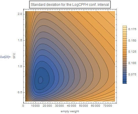
Figure 8 shows the standard deviation map for the construction of LogCPFH confidence intervals. The highest precision for mean CPFH predictions is obtained when SFC ≈ 0.75 lb/(lbf∙h) or lb/(hp∙h) and empty weight ≈ 15000 lb.

3. Parametric Model Predictions for ‘Known’ and ‘Unknown’ Aircraft Types

3.1. Model Comparative Predictions for Various Types

3.1.1. Predictions on the Training Sample

Results from the comparison of mean CPFH and 95% CI for the training sample are shown at Figure 9 and

Table 6. Comparison of mean CPFH and 95% CI for the training sample. The figures indicate ‘times the mean CPFH of F-16 Block 52+.’

Aircraft	CPFH Lower Bound	CPFH Expected	CPFH Upper Bound
T-41D	0.11901211	0.16420763	0.22162284
A-109E	0.19990530	0.25036102	0.31012026
T-6A II	0.25249018	0.30355962	0.36225471
AB-205	0.27634370	0.32830309	0.38749658
B-212	0.30764429	0.35999624	0.41896993
PZL	0.33723845	0.39536636	0.46093791
AS-332C1	0.35547705	0.41073767	0.47240366
T-2E	0.43697559	0.50679004	0.58491362
GV	0.44894272	0.53734944	0.63862291
EMB-135BJ/LR	0.44230344	0.54767037	0.67142878
EMB-145H	0.44643551	0.55351426	0.67940476
A-7	0.55941742	0.63567511	0.71971577
CL-415	0.54352594	0.64380037	0.75778338
CL-215	0.59726742	0.69851969	0.81253214
C-27J	0.58484956	0.72391072	0.88720093
M-2000/-5	0.70287959	0.83413491	0.98354446
F-16 Block 50	0.80040814	0.99097233	1.21478042
F-16 Block 52+	0.80500314	1.00000000	1.22957677
F-16 Block 30	0.81828962	1.02648845	1.27337004
C-130H/B	0.87955200	1.14080188	1.45822407
RF-4E	1.01709601	1.28261782	1.59868855
F-4E AUP	1.01709601	1.28261782	1.59868855

.

3.1.2. Predictions on a Set of ‘Unknown’ Aircraft Types

A comparative application of mean CPFH predictions with 95% CI for a set of ‘unknown’ aircraft types is shown at Figure 10 and

Table 7. A comparative application of mean CPFH predictions with 95% CI for a set of ‘unknown’ aircraft types. The figures indicate ‘times the mean CPFH of F-16 Block 52+.’

Aircraft	CPFH Lower Bound	CPFH Expected	CPFH Upper Bound
P2002JF	0.06753461	0.10155222	0.14747995
RACER	0.27574280	0.32714039	0.38563437
AW189	0.33099377	0.38469385	0.44488060
HH-60W	0.43900130	0.50855135	0.58631201
M-346	0.45194200	0.51116159	0.57619763
A-10A	0.46891536	0.57069196	0.68872595
AV-8B	0.53926887	0.60547233	0.67777883
T-X	0.48855572	0.61262218	0.75969810
T-100	0.56187968	0.63154563	0.70769602
T-50	0.69523642	0.84927503	1.02840736
JAS-39	0.71724836	0.87968786	1.06914862
F/A-18C/D	0.86861590	1.06510753	1.29424863
Eurofighter	0.87437845	1.06688394	1.29056054
Rafale C	0.88019674	1.10117609	1.36269648
AC-130U	0.87930885	1.14038891	1.45758505
F-35A	0.99567786	1.25154867	1.55541068
J-31	1.03666736	1.31599161	1.65010582
F-15E	1.05604359	1.34694738	1.69611550
Su-27SK	1.09117401	1.38460952	1.73549656
Su-57	1.14592428	1.46794227	1.85568007
F-22A	1.24714749	1.64265811	2.12859570

.

3.2. Model Predictions for the F-35A

The Lockheed Martin F-35 Lightning II is a family of fifth generation, single-seat, single engine, stealth multirole fighters undergoing final development and testing. It is intended to replace a plethora of existing aircraft types in the US Air Force, Navy and Marine Corps, while offering the most technologically advanced, effective and survivable fighter aircraft to date. The F-35 program, also known as the Joint Strike Fighter (JSF), is the most expensive weapon system in history with a projected service life up to 2070 and estimated sustainment costs of about $1 trillion [25]. The F-35 is designed and built by an industrial consortium led by Lockheed Martin. Besides the USA, many NATO members and close USA allied nations participate in the funding of the F-35 development. The US DoD plans to procure nearly 2500 aircraft [25] and several other countries have ordered, or are considering ordering the F-35.

Initial O&S cost estimates for the JSF date back to 2001 [26]. The focus of that study was to estimate the effect of changes in the reliability to the competition-sensitive O&S costs. As such, at the initial phases of the JSF development program it has been considered that reliability improvements have a strong effect on reducing O&S costs but not enough to recover initial investment. After the selection of the contractor has been made and the program has entered the production phase, the US DoD has moved on (2012) to establish affordability targets for the program, stating that the CPFH for the USAF, Marine Corps and US Navy could not exceed $35,200, $38,400 and $36,300 respectively [25].

The credibility of the O&S cost estimates and affordability targets made by the US DoD seem to have always been questionable though, not only for the F-35 [25] but for mature aircraft types as well [27]. As a general theme, the Government Accountability Office (GAO) recommends that the USAF and the Navy should follow all best practices [22,28] to improve the credibility of the CERs, including an investigation of the potential range of costs and, perhaps most importantly, seeking independent cost estimates. Research by GAO has shown that 19 out of 20 independent estimates developed by the Office of Secretary of Defence office of the Director of Cost Assessment and Program Evaluation were higher than the service (US Air Force, Navy) estimate. Past work of GAO has also shown that an independent estimate is usually higher and more accurate than an estimate, which has been made by the Program Office [29]. The present work also aims to serve the purpose of providing an independent estimate for various aircraft types and to constructively contribute to the current world-wide debate regarding the F-35 projected O&S costs. The developed parametric model predicts that the ratio of the mean CPFH of F-35A to the mean CPFH of the F-16C/D is 1.25. Figure 11 shows the cumulative distributions of the CPFH for the two systems.

4. Discussion

Developing sound O&S cost estimates for a new aircraft platform without data from its operational phase is a very demanding and complex process and possess significant, mainly non-systematic challenges for the aircraft operators, given that the CPFH estimates are affected by:

• Various operational variables and most importantly by the fleet utilization rates [2,3,4,10,11]. Many of those variables are often beyond the control of the aircraft operators, especially during situations (crisis, war conflicts) which require a sudden surge in aircraft flying hours.
• Reliability and maintainability improvements [2,30]. As above, the improvements are often beyond the control of the operators, they are mainly implemented during the production phase of the aircraft program and they are mainly based on best practices identified by analysing O&S data from historical aircraft projects. As such, there is uncertainty on the potential effect of a reliability and/or maintainability improvement to the O&S cost of a new aircraft program. The authors’ professional experience indicates, especially for aircraft types which are operated by many different users across the world (F-16C/D for example), that the implementation of an improvement at the aircraft production line or even later as a modification/upgrade, might not get necessarily translated into O&S cost savings, as different users develop different operational profiles for their fleets, to suit their specific operational needs.
• The ‘maturity’ of the fleet. In other words, by when the fleets are at their maximum size. This is because the ramp-up, steady-state and ramp-down phases tend to affect aircraft fleet cost [1].
• Inflation predictions, which are very difficult to estimate [13,14].

With regards to the developed parametric model, it is believed that it incorporates important features which enhance its ability to accurately predict the CPFH of an ‘unknown’ aircraft type:

• The aircraft sample is comprised by a well-balanced mix of fixed and rotary wing aircraft types which perform a plethora of different missions, from typical military nature (air defence and superiority, interception, aerial support to land and sea military operations) to public service nature ones (fire-fighting, search and rescue, air transportation of VIPs and equipment, medical evacuations). Despite the fact that a high degree of diversification exists in the training sample, a statistically significant CER was obtained consisting of the empty weight and the SFC. This CER seems realistic since both the SFC and aircraft weight are expected to be positively related with the energy consumed during a flying hour.
• The aircraft sample has reached maturity in terms of maximum fleet numbers and this is considered a very crucial condition for sound cost estimates, especially in case of comparing CPFH of different aircraft types [1]. Most of the aircraft sample types are legacy ones with stabilized CPFH, with the newest type (F-16C/D Block 52+Adv) approaching already ten years of operational life within the HAF.
• There is no significant variation of the utilization rates of the sample, mainly because of the fact that the engagement of HAF aircraft to war conflicts outside its national borders, conditions which require unpredictable aircraft utilization rate ‘spikes’ for prolonged periods of time, is minimal. The analysis of fleet data during the Operation Desert Storm and the operations at Kosovo [4,5] suggests that the CPFH proportional model fails when a fleet of aircraft significantly changes its flight behaviour from one time interval to the next (wartime surge for example). Furthermore, Boito et al. [1] suggest that the cost of fleets should be compared using stable annual flying hours required for crew proficiency, excluding flying hours for contingency operations. Of course, as many other NATO Air Forces, HAF actively conducts and participates in large scale military exercises within the country and abroad and there might be occasions in which the utilization rates would fluctuate but overall, they are considered as stable on an annual basis.

5. Conclusions

The accuracy of the cost estimates is also challenged by the variety and the complexity of the missions flown by the military operators. Commercial airline ‘cost per available seat mile’ is a widely used, simple and effective metric of cost and effectiveness, since fleets at the commercial industry are flown for a common and simple purpose which is easily measured. At the military field, there is a variety of missions and even within a given mission area, a military aircraft often provides many different capabilities. Hence, a ‘cost per capability’ shall be considered by the military operators as an additional metric for the O&S cost considerations of a military air platform. In such a metric, various capabilities and respective capability levels shall be defined for the fleet, which can then get adjusted on a cost basis. An application of the proposed methodology has been developed to optimize the maintenance of an aircraft system [31]. Recent evidence [25] has identified F-35 CPFH as being significantly higher than the legacy aircraft, with an F-35 Joint Program Office member of staff stating that ‘this was deemed reasonable taking into the account the complexity of the next-generation aircraft and the additional capability offered by the F-35’. The application of the parametric model for many ‘mature’ aircraft types for which there exists officially published CPFH data yields very promising results [10,11]. The calculated, by the parametric model, ratio (mean CPFH F-35A)/ (mean CPFH F-16 C/D) of 1.25 compares very well with the respective ratio of ‘normalized’ (CPFH F-35A)/ (CPFH F-16 C/D) of 1.27 (32,554/25,541 (2012$)) reported at the Selected Acquisition Reports (SARs) which have been submitted to the US Congress in 2013 [1]. Furthermore, the most recent available SAR estimate for the CPFH F-35 [32], which excludes the ‘indirect support’ contribution for both F-35 and F-16 C/D, calculates the ratio (CPFH F-35A)/(CPFH F-16 C/D) as 1.17 (29,806/25,541 (2012$)).

In general, it is believed that one of the key conclusions of the present work is that, not only the F-35A but also the majority of the new generation of the advanced fighter jets will not be significantly more costly to sustain than the F-16 C/D, when they will reach their ‘fleet maturity status.’ It is expected that the present work will inform the decision making and policy considerations of current F-16 C/D users who are considering acquiring a new generation advanced fighter jet fleet, especially in terms of financial forecasting, budgeting and planning of the optimum future force structure. It should also channel the existing debate to issues which relate to ‘cost per capability,’ given the promised enhanced capabilities which the F-35A is expected to offer as compared to previous generation fighter jet types.

References

1. Boito, M.; Keating, E.G.; Wallace, J.; DeBlois, B.; Blum, I. Metrics to Compare Aircraft Operating and Support Costs in the Department of Defense; Report number RR-1178-OSD; RAND Corporation: Santa Monica, CA, USA, 2015. [Google Scholar]
2. Hildebrandt, G.G.; Sze, M.B. An Estimation of USAF Aircraft Operating and Support Cost Relations; Report number N-2499-AF; RAND Corporation: Santa Monica, CA, USA, 1990. [Google Scholar]
3. Sherbrooke, C.C. Using Sorties vs Flying Hours to Predict Aircraft Spares Demand; Report number LMI-AF501LN1; Logistics Management Institute: McLean, VA, USA, 1997. [Google Scholar]
4. Wallace, J.M.; Houser, S.A.; Lee, D.A. A Physics-Based Alternative to Cost-Per-Flight-Hour Models of Aircraft Consumption Costs; Report number LMI-AF909T1; Logistics Management Institute: McLean, VA, USA, 2000. [Google Scholar]
5. Lee, D.A. The Cost Analyst’s Companion; Logistics Management Institute: McLean, VA, USA, 1997; ISBN 9780985396504. [Google Scholar]
6. Laubacher, M.E. Analysis and Forecasting of Air Force Operating and Support Cost for Rotary Aircraft; Biblioscholar, 2012; ISBN 9781288286126. Available online: https://www.bookdepository.com/Analysis-Forecasting-Air-Force-Operating-Support-Cost-for-Rotary-Aircraft-Matthew-E-Laubacher/9781288286126 (accessed on 2 October 2018).
7. Hawkins, J.C. Analysis and Forecasting of Army Operating and Support Cost for Rotary Aircraft. Master’s Thesis, Air Force Institute of Technology, Wright-Patterson Air Force Base, Dayton, OH, USA, 2004. [Google Scholar]
8. Armstrong, P.D. Developing an Aggregate Marginal Cost Per Flying Hour Model for the U.S. Air Force’s F-15 Fighter Aircraft; Biblioscholar, 2012; ISBN 9781288335183. Available online: https://www.bookdepository.com/Developing-an-Aggregate-Marginal-Cost-Per-Flying-Hour-Model-for-the-US-Air-Forces-F-15-Fighter-Aircraft-Patrick-D-Armstrong/9781288335183 (accessed on 2 October 2018).
9. Hess, T.J. Cost Forecasting Models for the Air Force Flying Hour Program. Master’s Thesis, Air Force Institute of Technology, Wright-Patterson Air Force Base, Dayton, OH, USA, 2009. [Google Scholar]
10. Hawkes, E.M.; White, E.D. Predicting the cost per flying hour for the F-16 using programmatic and operational data. J. Cost Anal. Manag. 2007, 9, 15–27. [Google Scholar] [CrossRef]
11. Hawkes, E.M.; White, E.D. Empirical evidence relating aircraft age and operating and support cost growth. J. Cost Anal. Parametr. 2008, 1, 31–43. [Google Scholar]
12. Unger, E.J. An Examination of the Relationship between Usage and Operating-and-Support Costs of U.S. Air Force Aircraft; Document number TR-594-AF; RAND Corporation: Santa Monica, CA, USA, 2009. [Google Scholar]
13. Smirnoff, J.P.; Hicks, M.J. The impact of economic factors and acquisition reforms on the cost of defense weapon systems. Rev. Financ. Econ. 2008, 17, 3–13. [Google Scholar] [CrossRef] [Green Version]
14. Christensen, D.S.; Searle, D.A.; Vickery, C. The Impact of the Packard Commission’s Recommendations on Reducing Cost Overruns on Defense Acquisition Contracts; Department of the Air Force: Washington, DC, USA, 1999. [Google Scholar]
15. McNutt, R. Reducing DoD Product Development Time: The Role of the Schedule Development Process. Ph.D. Thesis, Massachusetts Institute of Technology, Cambridge, MA, USA, 1998. [Google Scholar]
16. Office of the Secretary of Defense, Cost Assessment and Program Evaluation (OSD CAPE). Operating and Support Cost-Estimating Guide; Office of the Secretary of Defense: Washington, DC, USA, 2014. [Google Scholar]
17. Bozoudis, M. Case study: A parametric model for the Cost Per Flying Hour. In Proceedings of the ICEAA International Training Symposium, Bristol, UK, 17–20 October 2016. [Google Scholar]
18. International Society of Parametric Analysts. Parametric Estimating Handbook, 4th ed.; International Society of Parametric Analysts: Vienna, VA, USA, 2008. [Google Scholar]
19. Defense Acquisition University. Integrated Defense Acquisition, Technology, and Logistics Life Cycle Management Framework Chart, v5.2; Defense Acquisition University: Fort Belvoir, VA, USA, 2008. [Google Scholar]
20. Office of the Secretary of the Air Force. Technical Order 00-20-2: Maintenance Data Documentation, (Change 2-2007), Appendix L: “Air Force Standard Algorithms; Office of the Secretary of Defense: Washington, DC, USA, 2016. [Google Scholar]
21. Office of the Secretary of the Air Force. United States Air Force Cost Risk and Uncertainty Analysis Handbook (2007), par. 2.2.2.1 and 2.2.2.3.; Office of the Secretary of Defense: Washington, DC, USA, 2007. [Google Scholar]
22. United States Government Accountability Office. Cost Estimating and Assessment Guide: Best Practices for Developing and Managing Capital Program Costs; GAO-09-3SP; United States Government Accountability Office: Washington, DC, USA, 2009. [Google Scholar]
23. Hellenic Air Force (HAF) Official Web Site. Available online: www.haf.gr (accessed on 19 August 2018).
24. Bryant, M.T. Forecasting the KC-135 Cost per Flying Hour: A Panel Data Analysis. Master’s Thesis, Air Force Institute of Technology, Wright-Patterson Air Force Base, Dayton, OH, USA, 2007. [Google Scholar]
25. United States Government Accountability Office. F-35 Sustainment: Need for Affordable Strategy, Greater Attention to Risks, and Improved Cost Estimates; Report GAO-14-778; United States Government Accountability Office: Washington, DC, USA, 2014. [Google Scholar]
26. Birkler, J.; Graser, J.C.; Arena, M.V.; Cook, C.R.; Lee, G.; Lorell, M.; Smith, G.; Timson, F.; Younossi, O. Assessing Competitive Strategies for the Joint Strike Fighter: Opportunities and Options; Report number MR-1362.0-OSD/JSF; RAND Corporation: Santa Monica, CA, USA, 2001. [Google Scholar]
27. United States Government Accountability Office. Fighter Aircraft: Better Cost Estimates Needed for Extending the Service Life of Selected F-16s and F/A-18s; Report GAO-13-51; United States Government Accountability Office: Washington, DC, USA, 2012. [Google Scholar]
28. United States Government Accountability Office. Improvements Needed to Enhance Oversight of Estimated Long-Term Costs for Operating and Supporting Major Weapon Systems; GAO-12-340; United States Government Accountability Office: Washington, DC, USA, 2012. [Google Scholar]
29. United States Government Accountability Office. Defense Acquisitions: A Knowledge-Based Funding Approach Could Improve Major Weapon System Program Outcomes; Report GAO-08-619; United States Government Accountability Office: Washington, DC, USA, 2008. [Google Scholar]
30. Abell, J.B.; Kirkwood, T.F.; Petruschell, R.L.; Smith, G.K. The Cost and Performance Implications of Reliability Improvements in the F-16A/B Aircraft; Report number N-3062-ACQ; RAND Corporation: Santa Monica, CA, USA, 1988. [Google Scholar]
31. Bozoudis, M.; Lappas, I.; Kottas, A. Use of cost-adjusted importance measures for aircraft maintenance system maintenance optimization. Aerospace 2018, 5, 68. [Google Scholar] [CrossRef]
32. F-35 Lightning II Program Office. F-35 Lightning II Joint Strike Fighter (JSF) Program Selected Acquisition Report 2016; RCS: DD-A&T (Q&A) 823-198; F-35 Lightning II Program Office: Arlington, VA, USA, 2017. [Google Scholar]
Figure 1. Typical application of estimating techniques through a system’s life cycle stages [19].
Aerospace 05 00104 g001
Figure 2. Assessment of the linear model assumptions among the selected variables, using the global test on 4 degrees of freedom. The p-values lower than 0.05 (in red) indicate the rejection of linear model assumptions at the 5% significance level. It is evident that log-transformations enhanced linear relationships among variables.
Aerospace 05 00104 g002
Figure 3. The cluster dendrogram of the 22 systems.
Aerospace 05 00104 g003
Figure 4. The variables correlation (Pearson) matrix. The symbol “×” indicates the insignificant correlations at the 5% significance level. Multicollinearity is evident among several independent variables.
Aerospace 05 00104 g004
Figure 5. Visualization of the existing strong linear relationships between LogSPEED ~ AdjCEIL and LogMTOW ~ LogEMPTY.
Aerospace 05 00104 g005
Figure 6. 2D density plot (log-scale) for the model’s independent variables.
Aerospace 05 00104 g006
Figure 7. Typical residual plots.
Aerospace 05 00104 g007aAerospace 05 00104 g007b
Figure 8. The standard deviation map for the construction of LogCPFH confidence intervals.
Aerospace 05 00104 g008
Figure 9. Comparison of mean CPFH and 95% CI for the training sample.
Aerospace 05 00104 g009
Figure 10. A comparative application of mean CPFH predictions with 95% CI for a set of ‘unknown’ aircraft types.
Aerospace 05 00104 g010
Figure 11. The cumulative distribution for the F-35A CPFH compared to the F-16C/D Block52+, according to the developed parametric model.
Aerospace 05 00104 g011